| Issue |
A&A
Volume 566, June 2014
|
|
|---|---|---|
| Article Number | A57 | |
| Number of page(s) | 9 | |
| Section | Galactic structure, stellar clusters and populations | |
| DOI | https://doi.org/10.1051/0004-6361/201423419 | |
| Published online | 11 June 2014 | |
Numerical self-consistent distribution function of flattened ring models
Centro de Ciências Naturais e Humanas, Universidade Federal do
ABC,
09210-170
Santo André,
São Paulo,
Brazil
e-mail: This email address is being protected from spambots. You need JavaScript enabled to view it.
; This email address is being protected from spambots. You need JavaScript enabled to view it.
; This email address is being protected from spambots. You need JavaScript enabled to view it.
Received:
14
January
2014
Accepted:
31
March
2014
Abstract
We provide numerical, self-consistent distribution functions for several flat ring models by simultaneously solving the Fokker-Planck equation and the Poisson equation. In particular, we calculated the distribution function of flat ring systems formed by superposing Kuzmin-Toomre disc solutions and an analytic homogeneous ring solution in terms of complete elliptic integrals. We used these geometrical disc solutions, together with physical parameters, to model more realistic physical systems. Moreover, we defined a cutoff radius to handle the infinite Kuzmin-Toomre disc families numerically. The Fokker-Planck equation is solved by a direct numerical method using the finite difference method, the left conjugate direction algorithm, and a simple boundary condition that allows us to find good results for a large set of physical parameters and for values of the collision term of the same order of magnitude (or larger) when compared with the other terms in the Fokker-Planck equation. The collision term of the Fokker-Planck equation is explicitly calculated by applying the known Rosenbluth potentials for gravitational encounters. Limitations of the method are also discussed.
Key words: galaxies: kinematics and dynamics / methods: numerical
© ESO, 2014
1. Introduction
The importance of stationary solutions to the Boltzmann or Fokker-Planck equations for stellar objects or other systems is that they provide a starting point for dynamical evolutions and a way to study, analytically or numerically, the stability of the corresponding system. Furthermore, from the distribution function of a system, we can obtain its thermodynamic variables by allowing a full understanding of the physics of each individual model. Many such studies have been conducted over the years (see e.g. Cohn 1979; Watanabe et al. 1981; Nishida et al. 1984; Yepes & Domínguez-Tenreiro 1992; Takahashi 1995; Theuns 1996; Takahashi et al. 1997; Joshi et al. 2001; Ashurov 2004; Fiestas & Spurzem 2010). Owing to the nature of the problem, the equations are usually solved numerically with approximative methods such as Monte Carlo (statistics) and moment equations (averages). On the other hand, direct numerical methods are not frequently considered, because of their computational complexity in two and three dimensions (Ujevic & Letelier 2005, 2006). Analytical solutions of the collisionless Boltzmann equation for thin discs were given in Mestel (1963) and Kalnajs (1972).
Regardless the importance of the Kalnajs and Mestel thin discs, we have to keep in mind that they do not model a realistic physical situation because they exhibit odd behaviours within the disc. Namely, in the Kalnajs discs, the distribution function goes to infinity for certain values of the energy density and the angular momentum; while in the Mestel discs, the gravitational potential Φ diverges at the centre of the disc. Thus, the problem of finding self-consistent stellar models for galaxies starting from known well-behaved gravitational potential models is of broad astrophysical interest. However, the procedure for finding reasonable physical models (either analytical or numerical) of the complete Fokker-Planck equation is not a simple task.
The main goal of our work is to use a direct numerical method to find self-consistent planar ring models that satisfy the Fokker-Planck equation and the Poisson equation and to study some of their properties. In many astrophysical systems, light is emitted by a thin stellar disc, thus our study of planar galaxies or planar systems is more than academically interesting. From the variety of gravitational ring models that have been proposed in the literature, we are going to focus on families of analytic ring models of Vogt & Letelier (2009) and the analytic homogeneous ring solution of Lass & Blitzer (1983). In the formulation of the Fokker-Planck equation, we include the collision term of the local approximation and calculate the diffusion coefficients as prescribed by Rosenbluth et al. (1957). Furthermore, based on the mass density profile of each particular model, a simple boundary condition for the Fokker-Planck equation has been successfully applied. To our knowledge, there has been no analytical or numerical solution of the Fokker-Planck equation for flat systems with rings.
The article is organized as follows. Section 2 introduces the Fokker-Planck equation for a thin disc with the collision term given by the local approximation and the diffusion coefficients. In Sect. 3, the computational code used to solve the Fokker-Planck equation is briefly explained. Section 4, presents the properties of the flattened ring models used in this article and the numerical results obtained. Finally, in Sect. 5, our results are summarized.
2. Fokker-Planck equation for flat systems with rings
To obtain a physical self-consistent model for an astrophysical system, its distribution
function f must
satisfy the Fokker-Planck equation and the Poisson equation simultaneously in a given time
t, say,
![Mathematical equation: \begin{eqnarray} \label{fp}&&\frac{\partial f}{\partial t} + \vec{v} \cdot \nabla f - \nabla \Phi \cdot \nabla_v f = \Gamma[f], \\ \label{poisson}&&\nabla^2 \Phi = 4 \pi G m \int f {\rm d}^3 v, \end{eqnarray}](/articles/aa/full_html/2014/06/aa23419-14/aa23419-14-eq4.png) where
v represents the velocity of the particles
(e.g. stars), ∇ is the usual
gradient, ∇v is the gradient in the velocity space
(derivatives with respect to the velocities), G the gravitational constant, Φ is the gravitational potential,
m the mass of
each particle, and the symbol Γ [f] represents the Fokker-Planck collision term. The
collision term in the local approximation has the form
where
v represents the velocity of the particles
(e.g. stars), ∇ is the usual
gradient, ∇v is the gradient in the velocity space
(derivatives with respect to the velocities), G the gravitational constant, Φ is the gravitational potential,
m the mass of
each particle, and the symbol Γ [f] represents the Fokker-Planck collision term. The
collision term in the local approximation has the form ![Mathematical equation: \begin{equation} \Gamma[f] = - \sum_{i=1}^3 \frac{\partial}{\partial v^i} \left[f D\left(\Delta v^i\right)\right] + \frac{1}{2} \sum_{i,j=1}^3 \frac{\partial^2}{\partial v^i \partial v^j} \left[f D\left(\Delta v^i \Delta v^j\right)\right], \label{gamma} \end{equation}](/articles/aa/full_html/2014/06/aa23419-14/aa23419-14-eq11.png) (3)where the functions
D(Δvi)
and D(ΔviΔvj)
are known as the diffusion coefficients.
(3)where the functions
D(Δvi)
and D(ΔviΔvj)
are known as the diffusion coefficients.
These coefficients were calculated (Rosenbluth et al. 1957) in the three-dimensional case by assuming an inverse square force for the interaction, and each stellar encounter involves only a single pair of stars and is independent of all others. These coefficients can be simplified if the field-star distribution function is described by a Maxwellian distribution (Binney & Tremaine 2008). We recall that the diffusion coefficients are calculated considering a test star of mass m moving through an infinite homogeneous sea of field stars of mass ma who has mean velocity equal to zero. The use of these coefficient in real actual systems, which are not homogeneous neither infinite, therefore have to be seen only as a first approximation. The reason for this simplification is that in general the diffusion coefficients also depend on the distribution function, so the Fokker-Planck equation is actually a more complicated integro-differential equation. Also, the diffusion coefficients are calculated by assuming encounters between the elements of the system and not collisions. (We use the word “encounter” to denote the gravitational perturbation of the orbit of one element of the system by another element, and the word “collision” to denote physical contact between elements. However, we keep “collision term” for the quantity Γ [f ].) Therefore, the results obtained in the following sections may not be valid in systems where collisions are important. Furthermore, the collision term is valid in the local approximation, which means that the encounter affects only the velocity and not the position of the interacting stars. For this reason strong deflections might be excluded.
Regarding the Fokker-Planck equation, it is important to mention that the individual stellar encounters gradually perturb stars away from their trajectories such that after many encounters, a star eventually loses track of its initial trajectory. The characteristic time interval in which these encounters are relevant to the evolution of the system corresponds to the relaxation time. The Fokker-Planck equation is appropriate for timescales exceeding the relaxation time, while the collisionless Boltzmann equation is appropriate for timescales lower than the relaxation time. It is known that encounters may have played an important part in the structure of stellar systems, such as globular clusters, galactic nuclei, open clusters nuclei, and clusters of galaxies.
Equations (1) and (2), together with the collision term (3) are valid for a general three-dimensional
case. As a first approximation in our study we consider a case of a very thin disc with
thickness approximately equal to δz ≈ 10-8% of the size of its radius and
stars with low velocities in the z direction. By taking these approximations into
account, we can rewrite the Fokker-Planck equation in cylindrical coordinates as
![Mathematical equation: \begin{equation} \frac{\partial f}{\partial t} \!+\! \dot{r} \frac{\partial f}{\partial r} \!+\! \dot{\varphi} \frac{\partial f}{\partial \varphi} + \left( \frac{v_\varphi^2}{r}\! -\! \frac{\partial \Phi}{\partial r} \right) \frac{\partial f}{\partial v_r} \!-\! \left( \frac{v_r v_\varphi}{r} + \frac{1}{r} \frac{\partial \Phi}{\partial \varphi} \right) \frac{\partial f}{\partial v_\varphi} = \Gamma[f], \label{fokker2d} \end{equation}](/articles/aa/full_html/2014/06/aa23419-14/aa23419-14-eq17.png) (4)with
(4)with ![Mathematical equation: \begin{equation} \Gamma[f] = - \sum_{i=1}^2 \frac{\partial}{\partial v^i} \left[f D\left(\Delta v^i\right)\right] + \frac{1}{2} \sum_{i,j=1}^2 \frac{\partial^2}{\partial v^i \partial v^j} \left[f D\left(\Delta v^i \Delta v^j\right)\right]. \label{gamma2d} \end{equation}](/articles/aa/full_html/2014/06/aa23419-14/aa23419-14-eq18.png) (5)The same result can
be obtain if we start with Eq. (1) and
perform a projection on the z =
0 and vz = 0 planes using
Dirac deltas, i.e. doing the replacement f(x,v,t)
→
f(x,v,t)δ(z)δ(vz)
and integrating in the z and vz variables (Ujevic & Letelier 2005). The explicit form of the
collision term Γ [f] is presented in Appendix A.
(5)The same result can
be obtain if we start with Eq. (1) and
perform a projection on the z =
0 and vz = 0 planes using
Dirac deltas, i.e. doing the replacement f(x,v,t)
→
f(x,v,t)δ(z)δ(vz)
and integrating in the z and vz variables (Ujevic & Letelier 2005). The explicit form of the
collision term Γ [f] is presented in Appendix A.
3. Numerical method
The general procedure for finding the self-consistent distribution function is the
following. First, we fix our system in a given time t, then we insert the
gravitational potential (Φ) of
our system into the Fokker-Planck equation. After that, we set the values of the physical
parameters for the model and the boundary conditions of the system. Then, we solve the
Fokker-Planck equation numerically to obtain the distribution function (f). Once we determine the
distribution function, we calculate the mass density numerically with the relation
 (6)To simplify the integration
in Eq. (6) we set the upper boundary velocity
in each domain point to be the maximum escape velocity of the whole system, i.e.
(6)To simplify the integration
in Eq. (6) we set the upper boundary velocity
in each domain point to be the maximum escape velocity of the whole system, i.e.
 , where
 .
Finally, we compare the numerical mass density obtained by Eq. (6) with the original analytical mass density,
which is associated with the gravitational potential inserted in the Fokker-Planck equation.
If both densities coincide, then we conclude that the distribution function is
self-consistent, and if they do not coincide, we modify the values of the physical
parameters and repeat the procedure until a self-consistent distribution function is
reached. When the desired distribution function is obtained, we can calculate the average
value of any observable
.
Finally, we compare the numerical mass density obtained by Eq. (6) with the original analytical mass density,
which is associated with the gravitational potential inserted in the Fokker-Planck equation.
If both densities coincide, then we conclude that the distribution function is
self-consistent, and if they do not coincide, we modify the values of the physical
parameters and repeat the procedure until a self-consistent distribution function is
reached. When the desired distribution function is obtained, we can calculate the average
value of any observable  as a function of r by using
 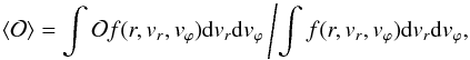 (7)where
the integrals (6) and (7) are calculated numerically using the Simpson
1/3 method.
(7)where
the integrals (6) and (7) are calculated numerically using the Simpson
1/3 method.
We discretized the Fokker-Planck equation by applying a finite differencing method, which uses a central-differences second-order scheme for the first and the second-order partial derivatives. In this work, the gravitational potentials are axially symmetric, therefore the distribution function f depends on three variables: one spatial variable (r) and two velocity variables (vr and vϕ). We therefore used an eleven-point discretization molecule. (The mixed derivatives of Γ [f ] in Eq. (5) introduce a more complex discretization molecule.) We used a grid of 51 nodes for the r variable and 25 nodes for each velocity variable.
After the discretization, the resulting system of linear algebraic equations is solved
using the robust left conjugate direction method (Catabriga
et al. 2004). The boundary condition for our problem must have a spatial part and a
velocity part. An appropriate boundary condition for the velocity part can be found if we
recall that the velocity distribution in a star system is determined by two competing
processes: there is the relaxation through the stellar encounters that drives the
distribution toward a Maxwellian form, and on the other hand, there are stars that, by going
beyond the finite escape velocity, continually disappear from the system. Since the escaping
stars traverse the system in a small fraction of a relaxation time, the resulting velocity
distribution should be zero beyond the escape velocity, but otherwise nearly Maxwellian.
Thus, we propose a Maxwellian distribution for the velocities at the border. Now, for the
spatial boundary condition we found that the best results are obtained when we set the
spatial part equal to the analytic mass surface density of the particular model evaluated at
the border. Therefore, we set the boundary condition at the border of the system as
![Mathematical equation: \begin{equation} f_{\rm Boun}(r, v) \propto \exp{\left[ -v^2/2 \sigma^2_v\right]} \cdot \Sigma(r), \label{boundary} \end{equation}](/articles/aa/full_html/2014/06/aa23419-14/aa23419-14-eq31.png) (8)where Σ(r) is the analytical mass
surface density of the particular model, and σv is a constant with
velocity dimension.
(8)where Σ(r) is the analytical mass
surface density of the particular model, and σv is a constant with
velocity dimension.
With this computational setup we have obtained self-consistent solutions when the collision term is of the same order of magnitude (or bigger) as the larger term on the left-hand-side of Eq. (1). For lower values of the collision term, we start having problems finding self-consistent models. One computational problem is that when we decrease the values of the collision terms the discretization matrix (representing the system of linear equations) that we need to solve has low values in the main diagonal, and most of the computational methods fail to give us a correct (or accurate) solution for this case. Perhaps changing the discretization method or the numerical method used to invert the matrix will solve this problem. Also, we may have to consider more realistic diffusion coeficients for our systems. At the moment we are studying different alternatives that will be discussed elsewhere.
4. Flattened galactic ring model
4.1. Flat Kuzmin-Toomre family of rings
Recently, Vogt & Letelier (2009) have found a family of flat rings system (characterized by zero density on r = 0) and a family of a flat discs with rings using the superposition of the members of the Kuzmin-Toomre family of discs. All the models have axial symmetry and infinite extension, thus, to make the numerical calculations, we limit the extension of the systems by setting a cutoff radius (r = rmax). It is interesting that this family of solutions also admits a relativistic representation (Ujevic et al. 2011).
 |
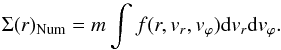
Fig. 1 Results for the ring (1,1). We consider the parameters a = 4 kpc, σ = 48.87 km s-1, ℳ(1,1) = 109 M⊙, ρ = 1.35 × 10⁻¹³ kg m-3, ma = M⊙, vtyp = 0.8σ, bm = 4 kpc, δz = 6 × 10⁻¹⁰ kpc, σv = 0.8σ, and rmax = 4a. In graph a) the mass surface density profile of the exact solution (solid line) is compared with the mass surface profile obtained from the numerical integration of Eq. (6) (full circles). In the region with the highest density, the difference between them is less than 0.8%. Graph b) shows the values of ⟨ v2 ⟩ /σ2 within the ring. Graphs c) and d) show the velocity distribution function and the level curves for case r/a ≈ 0.72, respectively. Graphs e) and f) show the spatial distribution function and the level curves for case vϕ = 0, respectively. |
4.1.1. Family of one-ring systems
The family of one-ring systems is defined by the mass surface density 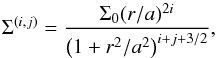 (9)where Σ0 is a constant with dimension
of mass surface density, a is a parameter of the model, i =
1,2,... and
j =
0,1,.... The
total mass ℳ(i,j) can be obtained by simply
integrating Σ(i,j) over the space. The
gravitational potentials associated to the density (9) can be calculated with the same coefficients as used in the
superposition of (9) (see Vogt & Letelier (2009) for details). For
example, if we take the (1,1) model (this corresponds to i = 1 and j = 1), the mass density
of the model is
(9)where Σ0 is a constant with dimension
of mass surface density, a is a parameter of the model, i =
1,2,... and
j =
0,1,.... The
total mass ℳ(i,j) can be obtained by simply
integrating Σ(i,j) over the space. The
gravitational potentials associated to the density (9) can be calculated with the same coefficients as used in the
superposition of (9) (see Vogt & Letelier (2009) for details). For
example, if we take the (1,1) model (this corresponds to i = 1 and j = 1), the mass density
of the model is 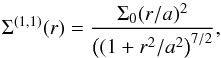 (10)and the respective
gravitational potential is (in z = 0)
(10)and the respective
gravitational potential is (in z = 0) 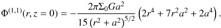 (11)Now, with (11) in the Eq. (4) we can find the distribution function of
the system, and then the numerical mass surface density using Eq. (6). For the outer boundary condition, we set
Eq. (8) and for the inner boundary
condition we set f =
0.
(11)Now, with (11) in the Eq. (4) we can find the distribution function of
the system, and then the numerical mass surface density using Eq. (6). For the outer boundary condition, we set
Eq. (8) and for the inner boundary
condition we set f =
0.
Figure 1 shows the numerical results for the single ring (1,1) with parameters a = 4 kpc, σ = 48.87 km s-1, ℳ(1,1) = 109M⊙, ρ = 1.35 × 10⁻¹³ kg m-3, ma = M⊙, vtyp = 0.8σ, bm = 4 kpc, δz = 6 × 10⁻¹⁰ kpc, σv = 0.8σ, and rmax = 4a. In Fig. 1a the mass surface density obtained after integrating (6) is compared with the exact mass density (10). The agreement between them is very good. Namely, in the densest part of the graph, near r/a ≈ 0.7, the biggest difference appears between them into account, which is less than 0.8%. If we take all the assumptions made so far and the fact that we are trying to match a real finite physical system to an infinite geometric potential that was developed without using any observational data, then the result is more than satisfactory.
With the help of the distribution function and Eq. (7) in Fig. 1b, the values of ⟨ v2 ⟩/σ2 within the ring are plotted, and this quantity is related with the temperature of the system. We see that the highest value of the temperature coincides with the densest region, the temperature drops to zero near the origin, and it is almost constant in the rest of the system. To get more complete information about the system, we present in Fig. 1c, d the velocity profile and the level curves of the distribution function for the value r/a ≈ 0.72, respectively, and in Fig. 1e, f the spatial profile and the level curves of the distribution function for the value vϕ = 0, respectively. The level curves of Fig. 1d move to the left for values of r/a< 0.72, and for values of r/a> 0.72, the level curves move to the right. In Fig. 1f the level curves are the same for different values of vϕ, changing only the magnitude of the distribution function. We performed several calculations of the single-ring model (1,1) with different values of ℳ(1,1) and a, finding self-consistent models for different physical parameters, given that we have properly chosen the values of σ and ρ. For instance, for vtyp = 0.8σ, bm ≈ a, rmax = 4a, and σv = 0.8σ, the self-consistency occurs when the parameters ℳ(1,1), ma, a, and δz satisfy the inequality ln [ 0.71(ℳ(1,1)/ma) ] ·(ma/ ℳ(1,1))·(a/δz) ≳ 102.19. After many calculations we have concluded that this inequality is only a limitation of the numerical method employed and not a physical limitation.
Besides the single-ring model (1,1) presented here, we also investigated different single-ring models (i,j) of Eq. (9) with good results.
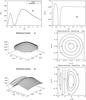 |
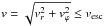
Fig. 2 Results for the double ring (1, 2). We consider the parameters a = 4 kpc,
σ =
24.80 km s-1, |
4.1.2. Family of double-ring systems
In this case, the family of double-ring systems is defined by the mass surface density
 (12)where κ is a dimensionless
nonzero constant. In these models a gap is placed at r/a = 1/κ, thus generating a family of
two concentric flat rings. As a study case we take the (1, 2) model. For this model, the
mass surface density is
(12)where κ is a dimensionless
nonzero constant. In these models a gap is placed at r/a = 1/κ, thus generating a family of
two concentric flat rings. As a study case we take the (1, 2) model. For this model, the
mass surface density is 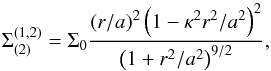 (13)and the respective
gravitational potential is (in z = 0)
(13)and the respective
gravitational potential is (in z = 0)
![Mathematical equation: \begin{eqnarray} \Phi^{(1,2)}_{(2)}(r,z=0) &=& -\frac{2\pi\Sigma_0 G a^2}{105\chi^{7/2}}\left\{6\chi^3\left(1+8\kappa^4\right)\phantom{\left(1+\kappa^2\right)^2} \right. \nonumber \\ &&+\, \chi^2\left[-16\kappa^2r^2 +a^2\left(9-26\kappa^2-54\kappa^4\right)\right]\nonumber \\ && -\,2a^2\chi\left[r^2\left(2+11\kappa^2+9\kappa^4\right)\right. \nonumber \\ &&\left.-\,a^2\left(7+28\kappa^2+21\kappa^4\right)\right] \nonumber \\ &&\left.-\,3a^4\left(1+\kappa^2\right)^2\left[2r^2+7a^2\right]\right\}, \end{eqnarray}](/articles/aa/full_html/2014/06/aa23419-14/aa23419-14-eq92.png) (14)where
χ =
r2 + a2.
For this family of rings we consider the same boundary conditions used in the
single-ring systems.
(14)where
χ =
r2 + a2.
For this family of rings we consider the same boundary conditions used in the
single-ring systems.
In Fig. 2 we present the numerical results for the
double-ring model (1,2) with parameters a = 4 kpc,
σ = 24.80
km s-1,
 , κ = 1.2, ρ = 0.12 ×
10-13 kg m-3, ma =
M⊙, vtyp =
0.8σ, bm = 4 kpc,
δz = 3 ×
10-9 kpc, σv =
0.8σ, and rmax = 4a. In Fig.
2a the mass surface density obtained after
integrating (6) is compared with the
exact mass surface density (13). The
biggest difference between them is less than 1.7%, and it occurs in the densest region.
This is again a good result for the same reasons as in the single-ring model. In Fig.
2b the quantity ⟨ v2 ⟩/σ2, which corresponds
to the temperature of the system, is plotted.
, κ = 1.2, ρ = 0.12 ×
10-13 kg m-3, ma =
M⊙, vtyp =
0.8σ, bm = 4 kpc,
δz = 3 ×
10-9 kpc, σv =
0.8σ, and rmax = 4a. In Fig.
2a the mass surface density obtained after
integrating (6) is compared with the
exact mass surface density (13). The
biggest difference between them is less than 1.7%, and it occurs in the densest region.
This is again a good result for the same reasons as in the single-ring model. In Fig.
2b the quantity ⟨ v2 ⟩/σ2, which corresponds
to the temperature of the system, is plotted.
The temperature drops to zero in the regions without particles, i.e. at the origin and at the intersection of the rings. The highest temperature is located in the inner ring, and in the outer ring the temperature is almost constant. For completeness, we present in Fig. 2c, d the velocity profile and the level curves of the distribution function for the value r/a ≈ 2.32, respectively. For values of r/a > 2.32, the level curves of Fig. 2d are nearly the same, for values of 0.37 < r/a < 0.80 the level curves move to the right and for other values of r the level curves move to the left. Moreover, in Fig. 2e, f we plot the spatial profile and the level curves of the distribution function for the value vϕ = 0, respectively. The level curves of Fig. 2f have the same profile for different values of vϕ, varying the magnitude of the distribution function.
We performed several calculations for the double-ring model (1, 2) with different
values of  ,
a, and
κ and
find self-consistent models, given again (as in the single-ring case) that we have
properly chosen the values of σ and ρ. As an example for the double – ring model, for
vtyp =
0.8σ, bm ≈
a, rmax = 4a,
σv =
0.8σ, and κ = 1.2, the self-consistency occurs when the
parameters ,
ma, a, and δz satisfy the inequality
,
a, and
κ and
find self-consistent models, given again (as in the single-ring case) that we have
properly chosen the values of σ and ρ. As an example for the double – ring model, for
vtyp =
0.8σ, bm ≈
a, rmax = 4a,
σv =
0.8σ, and κ = 1.2, the self-consistency occurs when the
parameters ,
ma, a, and δz satisfy the inequality
![Mathematical equation: \hbox{$\ln{[0.18(\mathcal{M}^{(1,2)}_{(2)}/m_a)]} \cdot (m_a/\mathcal{M}^{(1,2)}_{(2)}) \cdot (a/\delta z) \gtrsim 19$}](/articles/aa/full_html/2014/06/aa23419-14/aa23419-14-eq100.png) . For this case and as in the
previous section, the conclusion is that this inequality is only a limitation of the
numerical method employed and not a physical limitation.
. For this case and as in the
previous section, the conclusion is that this inequality is only a limitation of the
numerical method employed and not a physical limitation.
Besides the double-ring model (1, 2) discussed above, we went on to investigate different double- ring models (i,j) of Eq. (12) with similarly good results.
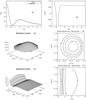 |
Fig. 3 Results for the disc with a ring for the i = 2 model. We
consider the parameters a = 4 kpc, σ = 29.74
km s-1,
|
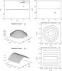 |
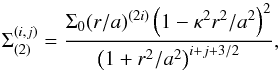
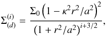
Fig. 4 Results for the homogeneous ring model. We consider the following parameters a = 10 kpc, b = 12 kpc, σ = 36.95 km s-1, ℳR = 109M⊙, ρ = 0.24 × 10⁻¹³ kg m-3, ma = M⊙, vtyp = 0.8σ, bm = 2 kpc, δz = 2 × 10⁻⁸ kpc, and σv = 0.9σ. In graph a) the mass surface density profile of the exact solution (solid line) is compared with the mass surface density profile obtained from the numerical integration of Eq. (6) (full circles). The highest difference between them is less than 2.2%. Graph b) shows the values of ⟨ v2 ⟩ /σ2 within the ring. Graphs c) and d) show the velocity distribution function and the level curves for the case r/a ≈ 1.09, respectively. Graphs e) and f) show the spatial distribution function and the level curves for the case vr = 0, respectively. |
4.1.3. Family of discs with flat rings
The family of discs with flat rings is defined by the mass surface density
 (15)where κ is a dimensionless
nonzero constant. This surface mass density represents a disc with radius
r/a = 1/κ and a flat ring between
1/κ<r/a <
∞. As a study case, we take the i = 2 model. For this
model, the mass surface density is
(15)where κ is a dimensionless
nonzero constant. This surface mass density represents a disc with radius
r/a = 1/κ and a flat ring between
1/κ<r/a <
∞. As a study case, we take the i = 2 model. For this
model, the mass surface density is  (16)and the respective
gravitational potential is (in z = 0)
(16)and the respective
gravitational potential is (in z = 0)
![Mathematical equation: \begin{eqnarray} \Phi^{(2)}_{(d)}(r,z\!=\!0) &=& -\frac{2\pi\Sigma_0 G a^2}{15\chi^{5/2}}\!\left\{\chi^2\left(3\!-\!4\kappa^2\right) \!+\! \chi\left[3a^2\!-\!4\kappa^2 a^2\!+\!8\kappa^4 r^2\right] \right. \nonumber \\ && \left. + a^2\left[- r^2 \left(1 + 2\kappa^2\right) + a^2\left( 2 + 4\kappa^2 + 3\kappa^4\right)\right]\right\}, \end{eqnarray}](/articles/aa/full_html/2014/06/aa23419-14/aa23419-14-eq122.png) (17)where
again χ =
r2 + a2.
(17)where
again χ =
r2 + a2.
In Fig. 3 we present the numerical results for the
model i = 2
of a disc with a ring for the parameters a = 4 kpc, σ = 29.74
km s-1,
 ,
κ = 1.5,
ρ = 0.21 ×
10-13 kg m-3, ma = M⊙, vtyp =
0.8σ, bm = 4 kpc,
δz = 2 ×
10-9 kpc, σv =
σ, and rmax = 4a. In Fig.
3a, the exact mass surface density (16) is compared with the numerical
integrated mass density (6). We find good
agreement between them, and the biggest difference is again in the densest region (less
than 2.0%). In Fig. 3b we plot the quantity
⟨ v2 ⟩/σ2 to measure the
temperature of the system. The temperature drops to zero in the intersection of the disc
with the ring where there are no particles. The highest temperature is in the central
disc, and the temperature is almost constant in the ring. Figure 3c, d present the velocity profile and the level curves of the
distribution function for the value r/a ≈ 0.24,
respectively, and in Fig. 3e, f the spatial profile
and the level curves of the distribution function for the value vr =
0 is plotted, respectively. In Fig. 3d, the level curves move to the right for values of r/a between
0.24
< r/a <
0.63 and to the left for other values of r. For different values
of vr, we obtain the
same profile of Fig. 3f, changing only their
magnitudes. We performed several calculations of the i = 2 model with
different values of
,
κ = 1.5,
ρ = 0.21 ×
10-13 kg m-3, ma = M⊙, vtyp =
0.8σ, bm = 4 kpc,
δz = 2 ×
10-9 kpc, σv =
σ, and rmax = 4a. In Fig.
3a, the exact mass surface density (16) is compared with the numerical
integrated mass density (6). We find good
agreement between them, and the biggest difference is again in the densest region (less
than 2.0%). In Fig. 3b we plot the quantity
⟨ v2 ⟩/σ2 to measure the
temperature of the system. The temperature drops to zero in the intersection of the disc
with the ring where there are no particles. The highest temperature is in the central
disc, and the temperature is almost constant in the ring. Figure 3c, d present the velocity profile and the level curves of the
distribution function for the value r/a ≈ 0.24,
respectively, and in Fig. 3e, f the spatial profile
and the level curves of the distribution function for the value vr =
0 is plotted, respectively. In Fig. 3d, the level curves move to the right for values of r/a between
0.24
< r/a <
0.63 and to the left for other values of r. For different values
of vr, we obtain the
same profile of Fig. 3f, changing only their
magnitudes. We performed several calculations of the i = 2 model with
different values of  ,
a, and
κ, again
finding self-consistent models for properly chosen values of σ and ρ. This time our example
shows that for vtyp = 0.8σ,
bm ≈
a, rmax = 4a,
σv =
σ, and κ = 1.5, the self-consistency occurs when the
parameters ,
ma, a, and δz satisfy the inequality
,
a, and
κ, again
finding self-consistent models for properly chosen values of σ and ρ. This time our example
shows that for vtyp = 0.8σ,
bm ≈
a, rmax = 4a,
σv =
σ, and κ = 1.5, the self-consistency occurs when the
parameters ,
ma, a, and δz satisfy the inequality
![Mathematical equation: \hbox{$\ln{[0.26(\mathcal{M}^{(2)}_{(d)}/m_a)]} \cdot (m_a/\mathcal{M}^{(2)}_{(d)}) \cdot (a/\delta z) \ga 27$}](/articles/aa/full_html/2014/06/aa23419-14/aa23419-14-eq132.png) . As in previous sections,
this inequality should only be a limitation of the numerical method. Furthermore, good
results were obtained for different i models of Eq. (15).
. As in previous sections,
this inequality should only be a limitation of the numerical method. Furthermore, good
results were obtained for different i models of Eq. (15).
4.2. Homogeneous ring
In this section we consider an analytic homogeneous ring model written in terms of
complete elliptic integrals (Lass & Blitzer
1983). In this model, the ring has inner radius a, outer radius
b, and a
constant density Σ0, while the mass MR generates the gravitational potential
(written in cylindrical coordinates)
![Mathematical equation: \begin{eqnarray} \Phi(r,z = 0) &=& 2G\Sigma_0\left[(a+r)E( \eta_a)+(a-r)K(\eta_a)\right.\nonumber\\ &&\left.-\,(b+r)E( \eta_b)-(b-r)K( \eta_b)\right], \end{eqnarray}](/articles/aa/full_html/2014/06/aa23419-14/aa23419-14-eq136.png) (18)where
ηa =
4ar/ (a +
r)2, ηb =
4br/ (b +
r)2, and K and E are complete elliptic
integrals of the first and of the second order, respectively. The gravitational
acceleration can be written as
(18)where
ηa =
4ar/ (a +
r)2, ηb =
4br/ (b +
r)2, and K and E are complete elliptic
integrals of the first and of the second order, respectively. The gravitational
acceleration can be written as ![Mathematical equation: \begin{eqnarray} -\frac{\partial\Phi_{ba}}{\partial r} &=& 2 G\Sigma_0\left[( r + b)E(\eta_b)\left/r - \left(r^2 + b^2\right)\right. K(\eta_b)\left/\left(r^2 + br\right)\right. \right.\nonumber\\ &&\left.-\, (r + a)E( \eta_a)\left/r + \left(r^2 + a^2\right)\right. K( \eta_a)\left/\left(r^2 + ar\right)\right.\right], \end{eqnarray}](/articles/aa/full_html/2014/06/aa23419-14/aa23419-14-eq141.png) (19)where
we used the relations
(19)where
we used the relations  (20)The gravitational
acceleration has divergences at the boundary of the ring, i.e. in r = a and
r =
b, because the function K(η)
diverges when η =
1. To incorporate the radial acceleration in the Fokker-Planck equation
is necessary to calculate all the values of the function E(η) and
K(η). These functions will be
evaluated using Romberg’s integration scheme with a Richardson type of extrapolation. For
the inner ring and for the outer ring boundary condition, we again consider condition
(8).
(20)The gravitational
acceleration has divergences at the boundary of the ring, i.e. in r = a and
r =
b, because the function K(η)
diverges when η =
1. To incorporate the radial acceleration in the Fokker-Planck equation
is necessary to calculate all the values of the function E(η) and
K(η). These functions will be
evaluated using Romberg’s integration scheme with a Richardson type of extrapolation. For
the inner ring and for the outer ring boundary condition, we again consider condition
(8).
In Fig. 4 we present the numerical results for a homogeneous ring with parameters a = 10 kpc, b = 12 kpc, σ = 36.95 km s-1, ℳR = 109M⊙, ρ = 0.24 × 10⁻¹³ kg m-3, ma = M⊙, vtyp = 0.8σ, bm = 2 kpc, δz = 2 × 10⁻⁸ kpc, and σv = 0.9σ. In Fig. 4a the exact mass surface density (a constant) is compared with the numerical integrated mass density. We see that in the proximities of the borders of the ring, the calculated numerical density is less accurate than in the rest of the ring, and they show oscillatory behaviour. The error at the borders is less than 2.2%, thus the numerical integrated mass is in good agreement with the exact one considering that the gravitational acceleration has discontinuities at the borders. In Fig. 4b we plot the quantity ⟨ v2 ⟩/σ2. The temperature is almost constant within the ring, with some fluctuations in the vicinity of the borders possibly due to the boundary condition. Figure 4c,d shows the velocity profile and the level curves of the distribution function for the value r/a ≈ 1.09, respectively. For different values of r and vr, Fig. 4d and f have the same profiles, respectively. Finally, in Fig. 4e, f, we plot the spatial profile and the level curves of the distribution function for the value vr = 0.
Besides the model presented in Fig. 4 we performed several calculations with different values of ℳR, a, and b, and found self-consistent models for proper values of σ and ρ. For example, for vtyp = 0.8σ, bm ≈ a, b/a = 1.2, and σv = 0.9σ, the self-consistency occurs when the parameters ℳR, ma, a, and δz satisfy the inequality ln [0.20(ℳR/ma)] ·(ma/ℳR)·(a/δz) ≳ 2. As in previous sections, this inequality is only attributed to the limitation of the numerical method.
5. Conclusion
To obtain initial self-consistent data for the Fokker-Planck equation is, in general, not an easy task. In this work we found several solutions for systems of flat rings that satisfy the Fokker-Planck equation and the Poisson equation simultaneously. The collision term of the Fokker-Planck equation was obtained by taking the local approximation into account, while the diffusion coefficients were calculated following the work of Rosenbluth et al. (1957), where only gravitational encounters are taken into account. In particular, we found the distribution function of the flattened ring models of Vogt & Letelier (2009) and the flat homogeneous ring model of Lass & Blitzer (1983). It is interesting that we managed to model physical systems starting from geometric potentials that were developed without any observational data. To our knowledge, these are the first numerical solutions of the Fokker-Planck equation for flat systems with rings. Furthermore, it appears that the simple boundary condition used in our work gives good results for a large set of physical parameters. It will be very important to test this condition in different two-dimensional models and three-dimensional structures. Our results provide the basis needed for further evolution studies of the Fokker-Planck equation when different kinds of perturbations are applied.
Acknowledgments
C.A. thanks the CAPES for financial support, R.C. thanks the UFABC and CAPES for financial support, and M.U. thanks the CNPq for financial support.
References
- Ashurov, A. E. 2004, ApJ, 127, 2154 [NASA ADS] [Google Scholar]
- Binney, J., & Tremaine, S. 2008, Galactic Dynamics, 2nd edn. (Princeton, New Jersey: Princeton University Press) [Google Scholar]
- Catabriga, L., Coutinho, A. L. G. A., & Franca, L. P. 2004, Int. J. Numer. Meth. Eng., 60, 1513 [CrossRef] [Google Scholar]
- Cohn, H. 1979, ApJ, 234, 1036 [NASA ADS] [CrossRef] [Google Scholar]
- Fiestas, J., & Spurzem, R. 2010, MNRAS, 405, 194 [NASA ADS] [Google Scholar]
- Joshi, K. J., Nave, C. P., & Rasio, F. A. 2001, ApJ, 550, 691 [NASA ADS] [CrossRef] [Google Scholar]
- Kalnajs, A. J. 1972, ApJ, 175, 63 [NASA ADS] [CrossRef] [Google Scholar]
- Lass, H., & Blitzer, L. 1983, Celest. Mech. Dyn. Astron., 30, 225 [Google Scholar]
- Mestel, L. 1963, MNRAS, 126, 553 [NASA ADS] [CrossRef] [Google Scholar]
- Nishida, M. T., Watanabe, Y., Fujiwara, T., & Kato, S. 1984, PASJ, 36, 27 [NASA ADS] [Google Scholar]
- Rosenbluth, M. N., MacDonald, W. M., & Judd, D. L. 1957, Phys. Rev., 107, 1 [NASA ADS] [CrossRef] [MathSciNet] [Google Scholar]
- Takahashi, K. 1995, PASJ, 47, 561 [Google Scholar]
- Takahashi, K., Lee, H. M., & Inagaki, S. 1997, MNRAS, 292, 331 [NASA ADS] [CrossRef] [Google Scholar]
- Theuns, T. 1996, MNRAS, 279, 827 [NASA ADS] [CrossRef] [Google Scholar]
- Ujevic, M., & Letelier, P. S. 2005, A&A, 442, 785 [NASA ADS] [CrossRef] [EDP Sciences] [Google Scholar]
- Ujevic, M., & Letelier, P. S. 2006, J. Comput. Phys., 215, 485 [NASA ADS] [CrossRef] [Google Scholar]
- Ujevic, M., Letelier, P. S., & Vogt, D. 2011, Int. J. Mod. Phys. D, 20, 2291 [NASA ADS] [CrossRef] [Google Scholar]
- Vogt, D., & Letelier, P. S. 2009, MNRAS, 396, 1487 [NASA ADS] [CrossRef] [Google Scholar]
- Watanabe, Y., Inagaki, S., Nishida, M. T., Tanaka, Y. D., & Kato, S. 1981, PASJ, 33, 541 [NASA ADS] [Google Scholar]
- Yepes, G., & Domínguez-Tenreiro, R. 1992, ApJ, 387, 27 [NASA ADS] [CrossRef] [Google Scholar]
Appendix A: Explicit determination of the collision term
The collision term for the two-dimensional FP equation in the local approximation is
given by Eq. (5), where the diffusion
coefficients were determined by Rosenbluth in 1957 and have the following form
![Mathematical equation: \appendix \setcounter{section}{1} \begin{eqnarray} &&D[\Delta v_i] = 4 \pi G^2 m_a(m+m_a)\ln{\Lambda}\frac{\partial }{\partial v_i} \int d^3\vec{v}_a\frac{f_a(\vec{v}_a)}{|\vec{v}-\vec{v}_a|}, \nonumber \\ &&D[\Delta v_i\Delta v_j] = 4 \pi G^2 m^2_a \ln{\Lambda}\frac{\partial^2}{\partial v_i\partial v_j}\int d^3\vec{v}_a f_a(\vec{v}_a) |\vec{v}-\vec{v}_a|, \end{eqnarray}](/articles/aa/full_html/2014/06/aa23419-14/aa23419-14-eq153.png) (A.1)where
m and
ma are the mass of the
test particle and the field particle, respectively,
(A.1)where
m and
ma are the mass of the
test particle and the field particle, respectively,
 ,
vtyp is the typical velocity of the
particles in the system, and bm is the maximum
impact parameter. Numerical experiments show that the appropriate value for
bm is approximately the
orbital radius (Theuns 1996).
,
vtyp is the typical velocity of the
particles in the system, and bm is the maximum
impact parameter. Numerical experiments show that the appropriate value for
bm is approximately the
orbital radius (Theuns 1996).
The diffusion coefficients can be evaluated explicitly when the distribution function of
the field particles is known. The most important case is when the distribution function of
field particles is Maxwellian, i.e.
 (A.2)where
n is the
number density of particles, and σ the one-dimensional velocity dispersion of the
field particles. For this particular case, it is possible to find explicit expressions for
the diffusion coefficients
(A.2)where
n is the
number density of particles, and σ the one-dimensional velocity dispersion of the
field particles. For this particular case, it is possible to find explicit expressions for
the diffusion coefficients ![Mathematical equation: \appendix \setcounter{section}{1} \begin{equation} D[\Delta v_i] = \gamma\sigma\tilde{D}[\Delta\epsilon_i], \qquad D[\Delta v_i\Delta v_j] = \gamma\sigma^2\tilde{D}[\Delta\epsilon_i\Delta\epsilon_j], \label{cdif} \end{equation}](/articles/aa/full_html/2014/06/aa23419-14/aa23419-14-eq159.png) (A.3)where
(A.3)where
 ,
ρ =
nma,
ϵi =
vi/σ.
We define the new dimensionless diffusion coefficients
,
ρ =
nma,
ϵi =
vi/σ.
We define the new dimensionless diffusion coefficients
![Mathematical equation: \appendix \setcounter{section}{1} \begin{equation} \tilde{D}[\Delta\epsilon_i] = -\mathcal{A}(\epsilon)\epsilon_i, \qquad \tilde{D}[\Delta\epsilon_i\Delta\epsilon_j] = \frac{1}{\epsilon} \frac{\partial\mathcal{B}}{\partial\epsilon}\epsilon_i\epsilon_j + \mathcal{B}(\epsilon)\delta_{ij}, \end{equation}](/articles/aa/full_html/2014/06/aa23419-14/aa23419-14-eq163.png) (A.4)where
(A.4)where
 (A.5)Replacing
the expressions (A.3) in the collision
term (5), we find
(A.5)Replacing
the expressions (A.3) in the collision
term (5), we find![Mathematical equation: \appendix \setcounter{section}{1} \begin{equation} \Gamma[f]/\gamma = \!-\!\sum_{i=1}^{2}\!\frac{\partial}{\partial\epsilon_i} \Bigl\{f\tilde{D} [\Delta\epsilon_i]\Bigr\} \!+\! \frac{1}{2}\sum_{i,j=1}^{2}\! \frac{\partial^2}{\partial\epsilon_i\partial\epsilon_j}\Bigl\{f\tilde{D} [\Delta\epsilon_i\Delta\epsilon_j]\Bigr\}. \label{gamma2d-b} \end{equation}](/articles/aa/full_html/2014/06/aa23419-14/aa23419-14-eq165.png) (A.6)Evaluating the
derivatives we can write the previous equation as
(A.6)Evaluating the
derivatives we can write the previous equation as ![Mathematical equation: \appendix \setcounter{section}{1} \begin{equation} \Gamma[f]/\gamma = C_0 f \!+ \!C_1 \frac{\partial f}{\partial\epsilon_1} \!+\! C_2 \frac{\partial f}{\partial\epsilon_2} + C_{11}\frac{\partial^2 f} {\partial\epsilon^2_1} \!+\! C_{22}\frac{\partial^2 f}{\partial\epsilon^2_2} + C_{12}\frac{\partial^2 f}{\partial\epsilon_1\partial\epsilon_2}, \label{tcol-dim-c} \end{equation}](/articles/aa/full_html/2014/06/aa23419-14/aa23419-14-eq166.png) (A.7)where
(A.7)where ![Mathematical equation: \appendix \setcounter{section}{1} \begin{eqnarray} C_0 &=&\, \frac{1}{2}\tilde{D}[\Delta\epsilon_1\Delta\epsilon_1]_{,11} + \frac{1}{2}\tilde{D}[\Delta\epsilon_2\Delta\epsilon_2]_{,22} + \tilde{D}[\Delta\epsilon_1\Delta\epsilon_2]_{,12}\nonumber \\ &&-\, \tilde{D}[\Delta\epsilon_1]_{,1} - \tilde{D}[\Delta\epsilon_2]_{,2}, \nonumber\\ C_1 &=&\, \tilde{D}[\Delta\epsilon_1\Delta\epsilon_1]_{,1} + \tilde{D}[\Delta\epsilon_1\Delta\epsilon_2]_{,2} - \tilde{D}[\Delta\epsilon_1], \nonumber \\ C_2 &=& \,\tilde{D}[\Delta\epsilon_2\Delta\epsilon_2]_{,2} + \tilde{D} [\Delta\epsilon_2\Delta\epsilon_1]_{,1} - \tilde{D}[\Delta\epsilon_2], \nonumber\\ C_{11} &=& \,\frac{1}{2}\tilde{D}[\Delta\epsilon_1\Delta\epsilon_1], ~ C_{22}\! = \!\frac{1}{2}\tilde{D}[\Delta\epsilon_2\Delta\epsilon_2], ~ C_{12}\! =\! \tilde{D}[\Delta\epsilon_1\Delta\epsilon_2]. \label{coef-tcol} \end{eqnarray}](/articles/aa/full_html/2014/06/aa23419-14/aa23419-14-eq167.png) (A.8)Finally,
the derivatives of the dimensionless diffusion coefficients are determined from the
following relationships:
(A.8)Finally,
the derivatives of the dimensionless diffusion coefficients are determined from the
following relationships: ![Mathematical equation: \appendix \setcounter{section}{1} \begin{eqnarray} &&\tilde{D}[\Delta\epsilon_i]_{,i} \equiv \frac{\partial \tilde{D} [\Delta\epsilon_i]}{\partial \epsilon_i} = -\mathcal{A}-\epsilon^2_i \frac{1}{\epsilon}\frac{\partial \mathcal{A}}{\partial\epsilon}, \nonumber \\[-1mm] && \tilde{D}[\Delta\epsilon_i\Delta\epsilon_j]_{,i} = \epsilon^2_i\epsilon_j \left[\frac{1}{\epsilon}\frac{\partial}{\partial \epsilon}\right]^2 \mathcal{B} + (\epsilon_j+2\delta_{ij}\epsilon_i)\frac{1}{\epsilon} \frac{\partial\mathcal{B}}{\partial\epsilon}, \nonumber \\[-0.5mm] &&\tilde{D}[\Delta\epsilon_i\Delta\epsilon_j]_{,ij} = \epsilon^2_i \epsilon^2_j\left[\frac{1}{\epsilon}\frac{\partial}{\partial\epsilon} \right]^3 \mathcal{B} + (\epsilon^2_i+\epsilon^2_j+4\delta_{ij} \epsilon_i\epsilon_j)\left[\frac{1}{\epsilon} \frac{\partial}{\partial\epsilon}\right]^2\mathcal{B} \nonumber \\[-0.5mm] &&\qquad\qquad\qquad+\, (1+2\delta_{ij}) \frac{1}{\epsilon}\frac{\partial\mathcal{B}}{\partial\epsilon}, \label{dimlessdif} \end{eqnarray}](/articles/aa/full_html/2014/06/aa23419-14/aa23419-14-eq168.png) (A.9)
(A.9)
where ![Mathematical equation: \appendix \setcounter{section}{1} \begin{eqnarray} &&\frac{1}{\epsilon}\frac{\partial\mathcal{A}}{\partial\epsilon} = \mu \frac{-3\mbox{Erf}\left(\frac{\epsilon}{\sqrt{2}} \right)+\sqrt{\frac{2}{\pi}}\epsilon(\epsilon^2+3){\rm e}^{-\epsilon^2/2}} {\epsilon^5}, \nonumber \\ &&\frac{1}{\epsilon}\frac{\partial\mathcal{B}}{\partial\epsilon} = -\frac{(\epsilon^2-3)\mbox{Erf}\left(\frac{\epsilon} {\sqrt{2}}\right)+3\sqrt{\frac{2}{\pi}}\epsilon {\rm e}^{-\epsilon^2/2}} {\epsilon^5}, \nonumber \\ &&\left[\frac{1}{\epsilon}\frac{\partial}{\partial\epsilon}\right]^2 \mathcal{B} = \frac{3(\epsilon^2-5)\mbox{Erf} \left(\frac {\epsilon}{\sqrt{2}}\right) + \sqrt{\frac{2}{\pi}} \epsilon(2\epsilon^2+15){\rm e}^{-\epsilon^2/2}} {\epsilon^7}, \nonumber \\ &&\left[\frac{1}{\epsilon}\frac{\partial}{\partial\epsilon}\right]^3 \mathcal{B} = -\frac{15(\epsilon^2\!-\!7)\mbox{Erf} \left(\frac {\epsilon}{\sqrt{2}}\right) \!+ \!\sqrt{\frac{2}{\pi}} \epsilon(2\epsilon^4\!+\!20\epsilon^2\!+\!105){\rm e}^{-\epsilon^2/2}} {\epsilon^9}\!\cdot \nonumber \\ \end{eqnarray}](/articles/aa/full_html/2014/06/aa23419-14/aa23419-14-eq169.png) (A.10)In
the case where ϵ →
0, we replace in Eq. (A.9) the following limits
(A.10)In
the case where ϵ →
0, we replace in Eq. (A.9) the following limits
![Mathematical equation: \appendix \setcounter{section}{1} \begin{eqnarray} &&\lim_{\epsilon\rightarrow 0} \frac{1}{\epsilon}\frac{\partial\mathcal{A}}{\partial\epsilon} \rightarrow - \mu\frac{\sqrt{\frac{2}{\pi}}}{5}, \qquad \lim_{\epsilon\rightarrow 0} \frac{1}{\epsilon}\frac{\partial\mathcal{B}}{\partial\epsilon} \rightarrow -\frac{2\sqrt{\frac{2}{\pi}}}{15}, \nonumber \\ &&\lim_{\epsilon\rightarrow 0}\left[\frac{1}{\epsilon} \frac{\partial}{\partial\epsilon}\right]^2 \mathcal{B} \rightarrow \frac{2\sqrt{\frac{2}{\pi}}}{35}, \lim_{\epsilon\rightarrow 0}\left[\frac{1}{\epsilon} \frac{\partial}{\partial\epsilon}\right]^3 \mathcal{B} \rightarrow -\frac{2\sqrt{\frac{2}{\pi}}}{63}, \nonumber \\ &&\lim_{\epsilon\rightarrow 0}\mathcal{A} \rightarrow \mu \frac{\sqrt{\frac{2}{\pi}}}{3}, \qquad \lim_{\epsilon\rightarrow 0}\mathcal{B} \rightarrow \frac{2\sqrt{\frac{2}{\pi}}}{3}, \end{eqnarray}](/articles/aa/full_html/2014/06/aa23419-14/aa23419-14-eq171.png) (A.11)in
order to avoid numerical instabilities.
(A.11)in
order to avoid numerical instabilities.
All Figures
|
Fig. 1 Results for the ring (1,1). We consider the parameters a = 4 kpc, σ = 48.87 km s-1, ℳ(1,1) = 109 M⊙, ρ = 1.35 × 10⁻¹³ kg m-3, ma = M⊙, vtyp = 0.8σ, bm = 4 kpc, δz = 6 × 10⁻¹⁰ kpc, σv = 0.8σ, and rmax = 4a. In graph a) the mass surface density profile of the exact solution (solid line) is compared with the mass surface profile obtained from the numerical integration of Eq. (6) (full circles). In the region with the highest density, the difference between them is less than 0.8%. Graph b) shows the values of ⟨ v2 ⟩ /σ2 within the ring. Graphs c) and d) show the velocity distribution function and the level curves for case r/a ≈ 0.72, respectively. Graphs e) and f) show the spatial distribution function and the level curves for case vϕ = 0, respectively. |
| In the text | |
|
Fig. 2 Results for the double ring (1, 2). We consider the parameters a = 4 kpc,
σ =
24.80 km s-1, |
| In the text | |
|
Fig. 3 Results for the disc with a ring for the i = 2 model. We
consider the parameters a = 4 kpc, σ = 29.74
km s-1,
|
| In the text | |
|
Fig. 4 Results for the homogeneous ring model. We consider the following parameters a = 10 kpc, b = 12 kpc, σ = 36.95 km s-1, ℳR = 109M⊙, ρ = 0.24 × 10⁻¹³ kg m-3, ma = M⊙, vtyp = 0.8σ, bm = 2 kpc, δz = 2 × 10⁻⁸ kpc, and σv = 0.9σ. In graph a) the mass surface density profile of the exact solution (solid line) is compared with the mass surface density profile obtained from the numerical integration of Eq. (6) (full circles). The highest difference between them is less than 2.2%. Graph b) shows the values of ⟨ v2 ⟩ /σ2 within the ring. Graphs c) and d) show the velocity distribution function and the level curves for the case r/a ≈ 1.09, respectively. Graphs e) and f) show the spatial distribution function and the level curves for the case vr = 0, respectively. |
| In the text | |
Current usage metrics show cumulative count of Article Views (full-text article views including HTML views, PDF and ePub downloads, according to the available data) and Abstracts Views on Vision4Press platform.
Data correspond to usage on the plateform after 2015. The current usage metrics is available 48-96 hours after online publication and is updated daily on week days.
Initial download of the metrics may take a while.