| Issue |
A&A
Volume 566, June 2014
|
|
|---|---|---|
| Article Number | A5 | |
| Number of page(s) | 12 | |
| Section | Interstellar and circumstellar matter | |
| DOI | https://doi.org/10.1051/0004-6361/201322982 | |
| Published online | 29 May 2014 | |
Galactic interstellar turbulence across the southern sky seen through spatial gradients of the polarization vector
1
Leiden Observatory, Leiden University,
PO Box 9513
2300 RA,
Leiden,
The Netherlands
e-mail:
This email address is being protected from spambots. You need JavaScript enabled to view it.
2
ASTRON, the Netherlands Institute for Radio
Astronomy, Postbus
2, 7990AA
Dwingeloo, The
Netherlands
3
Radboud University Nijmegen, Heijendaalseweg 135, 6525 AJ
Nijmegen, The
Netherlands
4
Astronomy Department, University of Wisconsin,
475 N. Charter St. Madison,
WI 53711,
USA
5
CSIRO Astronomy and Space Science, PO Box 76,
NSW 1710
Epping,
Australia
6
International Centre for Radio Astronomy Research, M468,
University of Western Australia, Crawley
WA 6009,
Australia
7
CAASTRO: The ARC
Centre of Excellence for All-sky Astrophysics,
Australia
8
Sydney Institute for Astronomy, School of Physics A29, The
University of Sydney,
NSW 2006
Sydney,
Australia
9
SKA SA, 3rd Floor, The Park, Park Road, 7405
Pinelands, South
Africa
10
Department of Physics and Electronics, Rhodes
University, PO Box
94, 6140
Grahamstown, South
Africa
11
Harvard Smithsonian Center for Astrophysics, 60 Garden
street, Cambridge
MA
02138,
USA
12
INAF Osservatorio Astronomico di Cagliari, via della
Scienza, 09047
Selargius,
Italy
Received:
5
November
2013
Accepted:
26
March
2014
Abstract
Aims. Radio synchrotron polarization maps of the Galaxy can be used to infer the properties of interstellar turbulence in the diffuse magneto-ionic medium (MIM). In this paper, we investigate the normalized spatial gradient of linearly polarized synchrotron emission (|∇P|/|P|) as a tracer of turbulence, the relationship of the gradient to the sonic Mach number of the MIM, and changes in morphology of the gradient as a function of Galactic position in the southern sky.
Methods. We used data from the S-band Polarization All Sky Survey (S-PASS) to image the normalized spatial gradient of the linearly polarized synchrotron emission (|∇P|/|P|) in the entire southern sky at 2.3 GHz. The spatial gradient of linear polarization reveals rapid changes in the density and magnetic fluctuations in the MIM due to magnetic turbulence as a function of Galactic position. We made comparisons of these data to ideal MHD numerical simulations. To constrain the sonic Mach number (Ms), we applied a high-order moments analysis to the observations and to the simulated diffuse, isothermal ISM with ideal magneto-hydrodynamic turbulence.
Results. We find that polarization gradient maps reveal elongated structures, which we associate with turbulence in the MIM. Our analysis indicates that turbulent MIM is in a generally transonic regime. This result for the turbulent regime is more general than the ones deduced by the analysis of electron density variation data, because it is based on the stochastic imprints of the Faraday rotation effect, which is also sensitive to the magnetic field fluctuations. Filamentary structures are seen with typical widths down to the angular resolution, and the observed morphologies closely match numerical simulations and, in some cases, Hα contours. The |∇P|/|P| intensity is found to be approximately log-normal distributed. No systematic variations in the sonic Mach number are observed as a function of Galactic coordinates, which is consistent with turbulence in the WIM, as inferred by the analysis of Hα data. We conclude that the sonic Mach number of the diffuse MIM appears to be spatially uniform towards the Galactic plane and the Sagittarius-Carina arm, but local variations induced by nearby extended objects are also found.
Key words: ISM: general / ISM: magnetic fields / ISM: structure / radio lines: general / radio continuum: ISM
© ESO, 2014
1. Introduction
Galactic magnetic fields and matter (i.e. atoms, ions and molecules) spread between the stars constitute a complex dynamic plasma, known as the interstellar medium (ISM). The density and temperature of the particles and the magnitude of the fields are fundamental parameters that shape the structure of the interstellar environment and characterize its evolution. Earlier studies (for a review see e.g. Ferrière 2001; Cox 2005) have pointed out the presence of magnetohydrodynamic (MHD) turbulence in the ISM, which is responsible for the distribution and the dissipation of energy through a wide range of spatial scales. MHD turbulence is thought to play an essential role for many key interstellar processes (for a review see e.g. Elmegreen & Scalo 2004), including star formation (see Krumholz & McKee 2005; McKee & Ostriker 2007), cosmic ray propagation (see Schlickeiser 2011; Lazarian et al. 2011) and magnetic reconnection (see Lazarian & Vishniac 1999). Additionally, astrophysical MHD turbulence is an integral part of the dynamics of the Galaxy, providing a significant pressure (and energy density) to support the diffuse ISM (Boulares & Cox 1990).
Many efforts have been made over the past decades to characterize magnetic fields and turbulence in the ISM as well as their mutual dependence (see review by Burkhart & Lazarian 2012a). The presence of a turbulent cascade in the ISM was obtained by tracing density variations in the warm ionized medium (Armstrong et al. 1995; Chepurnov & Lazarian 2010). However, MHD turbulence is traced in the different phases of the ISM by several typical signatures, such as density, velocity (Pogosyan & Lazarian 2009; Chepurnov et al. 2010), and synchrotron intensity (Lazarian & Pogosyan 2012; Iacobelli et al. 2013) variations. Because observations of astrophysical MHD turbulence and magnetic fields are challenging, the fundamental parameters of ISM turbulence, such as the sonic and Alfvénic Mach numbers, the magnetic field structure and strength, the Prandtl and Reynolds numbers, and the physical scale of energy injection are still poorly constrained. Therefore observational studies of MHD turbulence in the ISM, combined with analytic predictions and numerical simulations, are essential. Radio observations are a fundamental tool for gaining insight into magnetic fields, the density of the ionized gas, and their turbulent fluctuations. In particular, radio polarization maps constitute a useful diagnostic for studying turbulence and magnetic fields in the diffuse, ionized ISM (see e.g. Wieringa et al. 1993; Gaensler et al. 2001; Haverkorn et al. 2004a,b; Schnitzeler et al. 2007). Surveys covering a large part of the sky add information on the spatial dependence of these fields as well. Previous surveys of the southern sky are affected by several limitations such as incomplete sky coverage (e.g. the survey at 2.4 GHz by Duncan et al. 1995, 1997), the absence of polarimetric data (e.g. the survey at 2.3 GHz by Jonas et al. 1985, 1998) as well as a limited angular resolution (e.g. the survey at 1.4 GHz by Testori et al. 2008). The S-band Polarization All Sky Survey (S-PASS) (Carretti et al. 2013) is a recent spectro-polarimetric survey of the entire southern sky carried out with the Parkes 64 m telescope at 2.3 GHz to diminish depolarization effects with respect to 1.4 GHz surveys. The use of the spatial gradient of the polarization vector to image the small-scale structure associated with ISM turbulence has been recently discovered by Gaensler et al. (2011) and exploited by Burkhart et al. (2012). They show how to map the magnetized turbulence in diffuse ionized gas from the gradient of the Stokes Q and U pseudo-vectors. In a 18 deg2 patch of the Galactic plane, they find an intricate filamentary network of discontinuities in gas density and magnetic field. In agreement with the result of (Hill et al. 2008) for the warm ionized medium, these authors find turbulence in the magneto-ionic medium (MIM) to be transonic, with a sonic Mach number Ms ≲ 2 and therefore weakly compressible. These results were partially derived from the ability of statistical moments to characterize the sonic Mach numbers from spatial gradient maps of linear polarization by testing the sensitivity of statistical methods to different regimes of turbulence. Analyses of Gaensler et al. (2011) and Burkhart et al. (2012) find correlations between the spatial morphology, the higher order moments of the distribution of the spatial gradients of polarized emission and the sonic and Alfvénic Mach number.
In this paper we present the first mapping of different regimes of turbulence in the diffuse, ionized ISM over the entire southern sky by applying the statistical moments analysis to several regions. In particular, by comparing the analysis of high order moments in both simulations of MHD turbulence and observations we search for spatial variations of the sonic Mach number. Galactic coordinates are used throughout the following sections.
In Sect. 2 we present an overview of both the data and the gradient method. In Sect. 3 we present the spatial gradient map of the polarization vector displaying an extended network of filaments, and in Sect. 4 different regimes of MHD turbulence in the ISM are characterized from the moment map analysis. Finally, we discuss our results and present conclusions in Sect. 6.
2. Data overview
The S-band Polarization All Sky Survey (S-PASS) is a single-dish polarimetric survey of the entire southern sky at 2.3 GHz, performed with the Parkes 64 m Radio Telescope and its S-band Galileo receiver, which is a circular polarization system suitable for Stokes Q and U measurements. S-PASS observational parameters are given in Table 1, while a description of S-PASS observations and analysis is given by Carretti et al. (2013, and in prep.). To realize absolute polarization calibration of the data, an innovative observing strategy based on long scans along the horizon towards the east and west of the Parkes telescope was adopted. A system temperature of about 20 K was reached, with an improvement of a factor of 2 with respect to the previous continuum survey at the same frequency (see e.g. Duncan et al. 1997). Another main feature of the survey is its high angular resolution; due to a telescope beam width of 8.9′, final maps were obtained with a beam of FWHM = 10.75′ with an improvement of about a factor of 4 with respect to a previous continuum all-sky survey at 1.4 GHz (see e.g. Reich 2001). The final maps of the Stokes parameters resulting from the S-PASS survey will be fully presented by Carretti et al. (2013, and in prep.). We used the Stokes Q and U maps to image the spatial gradients of the linearly polarized emission for our analysis of ISM turbulence.
Observational properties of S-PASS data.
2.1. Radio polarization gradients
Variations in polarized intensity and polarization angles of radio synchrotron radiation are related to magnetic turbulence in the ISM. However, both these quantities are not invariant to rotations and translations in the Q–U plane, e.g. due to Faraday rotation by a uniform foreground screen and incomplete interferometric sampling respectively, making their interpretation difficult. A new diagnostic to investigate the turbulent fluctuations in the ISM affecting the radio polarization measurements is the spatial gradient of the polarization vector (Gaensler et al. 2011).
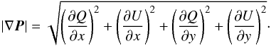
The radio polarization gradient (∇P) indicates the variation in the
polarization vector (P) as a function of position in the
image plane. In addition, the spatial gradient of the polarization vector acts as a
high-pass filter, allowing one to recover interesting features from a map with a strong DC
offset (see e.g. Schnitzeler et al. 2009). To
calculate the gradient of the polarization vector, we follow Gaensler et al. (2011), determining the magnitude as:
 (1)In general, fluctuations
in P are due to fluctuations in emission,
as well as fluctuations in Faraday rotation (Spangler
1982, 1983). However, in this paper we
treat the fluctuations in P as the result of stochastic
Faraday rotation due to Faraday screens on a polarized background. In this Faraday thin
approximation, the magnitude of the gradient of the polarization vector traces the Faraday
rotation changes from one line of sight to another, as modelled in Burkhart et al. (2012). We use correlation coefficients (see Sect. 4) to show that this approximation is justified for the
fields of view under consideration. Gradients in the polarization vector can be caused by
fluctuations in different quantities, as detailed below.
(1)In general, fluctuations
in P are due to fluctuations in emission,
as well as fluctuations in Faraday rotation (Spangler
1982, 1983). However, in this paper we
treat the fluctuations in P as the result of stochastic
Faraday rotation due to Faraday screens on a polarized background. In this Faraday thin
approximation, the magnitude of the gradient of the polarization vector traces the Faraday
rotation changes from one line of sight to another, as modelled in Burkhart et al. (2012). We use correlation coefficients (see Sect. 4) to show that this approximation is justified for the
fields of view under consideration. Gradients in the polarization vector can be caused by
fluctuations in different quantities, as detailed below.
-
1.
Fluctuations in Stokes I alone. Even in the case of no Faraday rotation or depolarization, variations in Stokes I will cause variations in the polarized intensity (|P|) and therefore a non-zero |∇P|. In this case, |P|∝ I and |∇P|∝ ∇I. Maps of |∇P| will act as an edge detection algorithm for fluctuations in synchrotron emission.
-
2.
Fluctuations in polarization angle alone. This is the case of a Faraday screen, which alters the direction of the polarization vector but not its amplitude. Then, |P|∝ I, but |∇P| is not correlated with either |P| or Stokes I. In this case, |∇P| directly traces gradients in rotation measure (RM), hence turbulence in the magneto-ionic ISM. This situation can be divided into two special cases:
-
a
A Faraday screen in front of spatially constant synchrotronemission. In this case, both Stokes I and |P| are constant, but |∇P| is not constant. Then (Burkhart et al. 2012),
 (2)and
the quantity |∇P|/|P| should be used to track
fluctuations in RM, i.e. to track magnetic turbulence. This is also the case in the
simulations we use to compare to the data.
(2)and
the quantity |∇P|/|P| should be used to track
fluctuations in RM, i.e. to track magnetic turbulence. This is also the case in the
simulations we use to compare to the data. -
b
The Faraday screen emits thermal, unpolarized radiation, such as an H ii region. In this case, some correlation between Stokes I and |∇P| may exist.
-
a
-
3.
Fluctuations in the polarized intensity and polarization angle, as caused by depolarization. In this case, Eq. (2) does not hold. Turbulence, as traced by |∇RM|, is tracked by |∇P|. This is the situation for which the polarization gradient method was originally created (Gaensler et al. 2011): RM fluctuations that cause depolarization canals are masked by foreground/background polarized emission, but the polarization gradient method makes these RM fluctuations visible even in the presence of a polarized emission foreground/background.
In the observations, gradients in the polarization vector will be caused by a combination of these three effects. In the following, we estimate the importance of each of these three effects by investigating correlations among Stokes I, polarized intensity |P|, and polarization gradient |∇P|. In fields where the Faraday screen approximation is reasonable, the normalized gradient map |∇P|/|P| traces fluctuations in RM. However, in fields where this approximation does not hold, the un-normalised map |∇P| should be considered.
Both the magnitude of the polarization spatial gradient (|∇P|) and of
the polarization vector (|P|) follow an asymmetric positive
distribution, while the Stokes Q and U parameters follow Gaussian distributions. The
positive definite distributions are signal-to-noise (S/N) dependent and are thus affected
by a bias towards high values at low S/N (Vinokur
1965). Wardle & Kronberg (1974)
suggested a widely used correction for the bias of a positive defined distribution
P(R) as
![Mathematical equation: \begin{equation} R \sim R_{\rm M}^{\prime} \left[1 - \left( \frac{\sigma^{\prime}}{R_{\rm M}^{\prime}} \right) \right]^{1/2} , \end{equation}](/articles/aa/full_html/2014/06/aa22982-13/aa22982-13-eq29.png) (3)where
(3)where
 is the
measured magnitude, σ′ the measured noise level, and
R the intrinsic magnitude of the signal vector. We confirmed the
Gaussian behaviour of Stokes Q and U maps and determined a noise level of
1 mJy beam-1 from a small region assumed to
contain no emission from the sky. We also assumed uniformity of the noise across the
entire field. Finally, we calculated the normalized gradient of the polarization vector
and discarded lines of sight where P is at the level of the bias
|PR| =
1.25σQ,U, resulting in a
fraction of blanked pixels of about 1% in the final |∇P|/|P| map.
is the
measured magnitude, σ′ the measured noise level, and
R the intrinsic magnitude of the signal vector. We confirmed the
Gaussian behaviour of Stokes Q and U maps and determined a noise level of
1 mJy beam-1 from a small region assumed to
contain no emission from the sky. We also assumed uniformity of the noise across the
entire field. Finally, we calculated the normalized gradient of the polarization vector
and discarded lines of sight where P is at the level of the bias
|PR| =
1.25σQ,U, resulting in a
fraction of blanked pixels of about 1% in the final |∇P|/|P| map.
To quantify the impact of the foreground Faraday rotation effects for these data, we
looked at the correspondence between total intensity and polarised intensity, by
determining the degree of correlation between the Stokes I and the |P| maps. If
the polarization signal is due to foreground Faraday rotation, little linear correlation
between the fluctuations of |P| and Stokes I is expected. Thus, we
adopted the Pearson correlation coefficient (ρp) defined as
 (4)where cov (P,I) is the covariance
and σP, σI are the standard
deviations of the Stokes I and the |P| maps. We considered the range of
weak correlation to be |ρp|≤ 0.35 and find a mild positive
correlation ρp =
0.38, so the bulk of the |∇P|/|P| fluctuations are not intrinsic to
the sources of polarized emission and can be interpreted in the framework of MHD
turbulence in the ionized ISM. In the following we select regions of low correlation where
the |∇P|/|P| fluctuations
can be interpreted in the framework of MHD turbulence.
(4)where cov (P,I) is the covariance
and σP, σI are the standard
deviations of the Stokes I and the |P| maps. We considered the range of
weak correlation to be |ρp|≤ 0.35 and find a mild positive
correlation ρp =
0.38, so the bulk of the |∇P|/|P| fluctuations are not intrinsic to
the sources of polarized emission and can be interpreted in the framework of MHD
turbulence in the ionized ISM. In the following we select regions of low correlation where
the |∇P|/|P| fluctuations
can be interpreted in the framework of MHD turbulence.
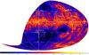 |
Fig. 1 Map of the normalised spatial gradient of linearly polarized emission, |∇P|/|P|, in Aitoff projection of the entire southern sky at a reference frequency of 2.3 GHz and a resolution of 11′. The noise level in the map was obtained by averaging intensity over a small region with no signal and intensity is clipped at 3σ. The scaling runs from 0.2 (black) to 1000 (white). Intensity unit is beam-0.5. |
3. Observational results
Figure 1 shows the final de-biased |∇P|/|P| sky map, clipped at 3σ for displaying purpose. The spatial gradient of the astrophysical polarized synchrotron emission of the diffuse Galactic foreground is depicted in this image at 2.3 GHz, producing a wealth of structures. Faint artefacts are also present around the equatorial south pole due to the scanning strategy. We now describe the main morphological features in the de-biased |∇P|/|P| map.
First, there are spatially compact and isolated structures, corresponding to bright extragalactic synchrotron sources. Several hundred unresolved sources (mostly quasars and radio galaxies) are detected to be smoothly distributed on the sky plane. Furthermore, a polarized extragalactic source showing a striking extended morphology is also present and marked in Fig. 1, the bright radio galaxy Cen A, with a north-south extension of about 8° of its structured emitting lobes.
There are also isolated Galactic structures on a range of scales. Peaks in the normalized polarization gradient signal are seen throughout the Galactic plane up to Galactic latitudes of |b| ≈ 25° corresponding to bright supernova remnants (SNRs) and nearby H ii regions. While the brightness of the former is mainly due to their intrinsic polarization, the latter are traced out by Faraday rotation along the line of sight to the observer induced by their thermal electrons. Indeed nearby (distance ~200 pc) and extended H ii regions are seen towards the inner Galaxy, such as Sh 2-27 around the O-class star ζ Ophiuchi (at l ~ 8°, b ~ 23°) and Sh 2-7 excited by the nearby star δ Sco (at l ~ 350°, b ~ 22°).
The outstanding characteristic is that most of the polarization gradients come from a network of filaments, which forms clearly separated and extended regions well outside the Galactic plane. The typical width of these filamentary structures matches the angular resolution. Furthermore, different morphological patterns of these filaments are seen. In Fig. 2 we show an example of the observed morphology for the normalized spatial gradients of polarized synchrotron emission, as a result of fluctuations in the MIM induced by different types of discontinuities (Burkhart et al. 2012). The panel depicts a complex region above the Galactic plane centred at (l,b) ≈ (278°, + 22°) and displays filamentary structures over a wide range of angular scales, up to about six degrees, with no correspondence to Stokes I. This extended pattern of filaments is due to the presence of discontinuities in the interstellar gas density and magnetic field. In particular, we note the presence of two evident structures that are also seen in MHD simulations (for a comparison see Fig. 4 of Burkhart et al. 2012) and are interpreted as due to different kinds of discontinuities in the warm, ionized ISM: a “double-jump” profile (box D) and a “single-jump” profile (box S), corresponding to the case of a (strong or weak) shock and a cusp or shear along the line of sight, respectively. Moreover changes in the |∇P|/|P| brightness along the filaments due to variations of the magnitude of turbulent fluctuations along the line of sight are recognized.
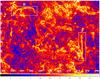 |
Fig. 2 A zoom of Fig. 1 centred on l ~ 278°, b ~ 22°, showing different observed morphologies for different MHD turbulence cases “double-jumps” (D boxed region) and “single-jump” (S boxed region) filaments due to (strong or weak) shocks and a cusps or shears along the line of sight, respectively. Intensity scale runs from 0.2 (black) to 2000 (white). |
Complex large-scale structures (such as the nearby and shell-like G 353-34) are seen up to intermediate (|b| ≈ 40°) Galactic latitudes. A prominent arc-like feature is observed within the longitude range 270° ≲ l ≲ 290°. The base of this magnetic structure is around l = 270°, and it extends up as an arc from the Galactic plane up to about (l,b) = (285°,45°) with an overall length of ~50°. Up to this point the structure is traced by the high polarization gradient intensity exhibiting a complex morphology: mostly filamentary at Galactic latitudes below 20° and mainly patchy, small-scale rich towards higher latitudes. High intensity values of radio polarization gradients are seen towards the third Galactic quadrant at high and negative Galactic latitudes, forming a very extended and patchy pattern up to b = −70° which is not spatially coincident with the nearby (d ≲ 500 pc) region of higher interstellar polarization pointed out by Berdyugin et al. (2004).
List of unambiguously identified SNRs in all of Stokes I, polarized intensity, and polarization gradient S-PASS maps, by cross-checking radio data taken from the Green (2009) database.
3.1. The polarization horizon
To constrain the impact of depolarization, to perform a proper comparison of data with numerical simulations, and to convert angular scales to spatial scales, we need to estimate the distance to which polarized emission is detected.
This spatial depth is referred to as the “polarization horizon”, and it has been used in previous works (see e.g. Landecker et al. 2002; Uyaniker et al. 2003). This quantity is a function of the instrumental features (i.e. the beam size, the observing frequency), as well as of the physical conditions of the probed medium (causing an intrinsic degree of depolarization). The smaller the beam and/or the higher the observing frequency, the farther the polarization horizon; the brighter and/or more coherent the synchrotron emission, the farther the corresponding polarization horizon. Recently, Carretti et al. (2013) have derived an estimate of about 2−3 kpc for the “polarization horizon” of these S-PASS data from the analysis of depolarized regions at low latitudes towards the inner Galaxy. However, the polarization horizon depends on the viewing direction in the Milky Way, and we consider the all-sky |∇P|/|P| intensity, so we need to find estimates for the maximum spatial depth up to intermediate Galactic latitudes (|b| ≲ 30°) and towards the outer regions (260° ≲ l ≲ 330°). To estimate a lower limit for the polarization horizon, we cross-checked the radio catalogue1 of Galactic SNRs (Green 2009) with detections in the Stokes I and |∇P|S-PASS maps, and we considered SNRs with a minimum angular size matching the S-PASS angular resolution. We used the |∇P| map because for sources with a large intrinsic polarization component, it acts as an edge detection algorithm, making the source detection towards regions with strong diffuse emission easier. Also, we note that the non-detection of polarization from a SNR may be due to internal depolarization in the SNR itself, constituting a limitation of the adopted method. Thus we decided not to use non-detections to constrain the upper limit of the polarization horizon.
We find four SNRs that satisfy our criteria (see Table 2) and suggest a lower limit for the polarization horizon about 3 kpc away from the Galactic centre, which agrees with the above estimate of Carretti et al. (2013) and is used throughout the following sections. At this distance, the presence of radio polarization gradient features down to an angular resolution of ~11′ corresponds to a linear scale of <10 pc for the filament widths, and therefore for the MIM fluctuations in the disk and the halo traced by these filaments. The earlier detection of |∇P|/|P| filaments at arcmin resolution by Gaensler et al. (2011), however, implies a typical width of ≈1 pc, if a polarization horizon of about 3 kpc is assumed for their data.
3.2. Galaxy-scale variations in |∇P| / |P|
The above lower limit of about 3 kpc for the polarization horizon constrains our data to probe the nearby, major large-scale Galactic features: the Local arm (Orion Spur) towards the outer region (i.e. 210° ≲ l ≲ 280°) and the Carina-Sagittarius arm located at a distance of about 2 kpc (Georgelin et al. 2000) between the Centaurus-Scutum spiral arm (~3.5 kpc) and the Sun towards the fourth Galactic quadrant. Also some emission from the nearest side of the Centaurus-Scutum spiral arm towards the Galactic center and the Perseus arm towards the outer region (i.e. l ≲ 250°) cannot be excluded. Moreover, out of the Galactic disk our estimate of about 3 kpc for the polarization horizon indicates a negligible amount of depolarization. Indeed, at Galactic latitudes |b| ≳ 45° this path length corresponds to a height ≳2.1 kpc, which is consistent with the scale heights of the relevant ISM components, the synchrotron-emitting thick disk (Beuermann et al. 1985; Kobayashi et al. 2004) and the scale height of the free electron density (Gaensler et al. 2008; Schnitzeler et al. 2012).
In this data set, regions of high |∇P|/|P| with no Stokes I correlation effectively trace the loci of compression or rarefactions of the magnetic fields and/or the warm ionized gas in the ISM, as well as abrupt changes in the direction of the magnetic field. Because the spiral arms constitute the most extended and synchrotron-emitting Galactic structures where these compressions and rarefactions take place, a spatial dependence of the |∇P|/|P| intensity with Galactic latitude and longitude is expected.
To focus on the diffuse emission, we mask the Galactic plane (|b| ≤ 2.5°) where depolarization effects are strong. The resulting map displays a diffuse foreground and a background consisting of extragalactic discrete sources and noise. We explore the dependence on Galactic latitude by looking at the distribution of the |∇P|/|P| intensity over four latitude ranges (see Fig. 3). The distribution peak position of the |∇P|/|P| intensities decreases with distance from the Galactic plane, but not the distribution width. In addition, the intensity counts are approximately represented by a log-normal distribution and the log-normal fit to the |∇P|/|P| intensity distribution of the latitude bin |b| ≲ 15°, which mostly probes the diffuse foreground emission, shows a reduced-χ2 of 2.09. Increasing deviations from a log-normal distribution are found with Galactic latitude.
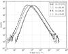 |
Fig. 3 Distributions of the |∇P|/|P| intensity of the masked map at four ranges of Galactic latitude (|b|). Statistical errors in each intensity bin are also shown. |
We highlight the presence of a longitude dependence of the |∇P|/|P| emissivity by using the first two moments (i.e. the mean and standard deviation) of the |∇P|/|P| distribution. We select lines of sight out of the Galactic disk over the latitude range 5° ≲ |b| ≲ 10° to limit the impact of depolarization. We sample the range of Galactic longitude with 5° sized squared bins, from which the mean and standard deviation of the |∇P|/|P| intensity are calculated and displayed in Fig. 4. We use the mean and standard deviation of |∇P|/|P| map as tracers of the diffuse emission and the presence of compact sources (e.g. SNRs, H ii regions), respectively. Both the profiles are characterized by the presence of peaks corresponding to nearby extended structures (e.g. the Vela SNR), as well as large-scale Galactic structures (e.g. the Carina-Sagittarius spiral arm), and a longitude dependence is seen with mean value of the normalized polarization gradient gradually decreasing towards the outer region. Towards the anti-centre (i.e. l ≲ 240°), no relevant diffuse emission is detected and few compact sources are seen. These directions mostly probe the Local-arm synchrotron diffuse emission, so both the |∇P|/|P| mean and standard deviation have low values, perhaps due to depolarization of the far end of the arm. A sudden jump in both moments is found around l ~ 260°, corresponding to the extended and nearby Gum Nebula and Vela SNR complex. Two minima are seen at lMIN,0 = (277.5° ± 2.5°) and lMIN,1 = (327.5° ± 2.5°), corresponding to the observed tangential directions (see Table 2 of Vallée 2008) of the Carina (282° ± 2°) and Norma (328° ± 3°) spiral arms. The low values of the mean and standard deviation may be explained by depolarization of the far end of the arms or by the alignment between the line of sight and the direction of the large-scale magnetic field. The latter option would imply a drop in the synchrotron emissivity.
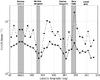 |
Fig. 4 Mean (solid lines) and standard (dashed lines) deviation profiles towards the Galactic disk (5° ≲|b|≲ 10°) for the |∇P|/|P| intensity as a function of Galactic longitude. The ranges of Galactic longitudes corresponding to the main Galactic features and spiral arms are also indicated. Data points are obtained from square regions of size 5°. |
3.3. Thermal electron density and magnetic features
The presence of Faraday rotation effects in these data are evident when comparing the |∇P|/|P| map with the Hα map. In this way it is possible to highlight (nearby) extended structures with relevant density and/or magnetic fluctuations. To this aim, we use the all-sky Hα map of Finkbeiner (2003), which has an angular resolution (of 6′) similar to that of the |∇P|/|P| map. We now report on some structures induced by density and/or magnetic fluctuations.
3.3.1. Nearby H ii regions
Nearby H ii regions are extended objects with prominent electron density fluctuations, for which a correspondence with Hα intensity is expected. Indeed a clear correlation of the |∇P|/P| and Hα intensity patterns is seen towards the nearby H ii regions Sh 2-27 and Sh 2-7, as shown in Fig. 5. The Hα intensity contours clearly trace features with higher |∇P|/|P| intensity both at the edges and towards the centre. A weak radio continuum feature is only seen for Sh 2-27, and the degree of correlation between the |∇P|/P| and the Stokes I intensity is |ρp|= 0.30,0.53 for Sh 2-27 and Sh 2-7, respectively. The higher degree of correlation found towards Sh 2-7 can be explained by the overlapping with the Galactic central spur, a feature detected with S-PASS in Stokes I and polarization (Carretti et al. 2013), and possibly emanating from the Galactic centre. The interpretation of the observed morphology in terms of ISM turbulent fluctuations is therefore supported only for Sh 2-27. This bubble-like feature is crossed and filled by filaments exhibiting a “single-jump” morphology, itself suggesting the presence of weak shock and/or strong turbulent fluctuations (Burkhart et al. 2012).
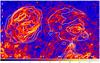 |
Fig. 5 Bubble-like |∇P|/|P| morphology of the nearby H ii regions Sh 2-27 (on the left) and Sh 2-7 (on the right) shown together with the contours of the Hα intensity from the all-sky map of Finkbeiner (2003). The units of contours are 1, 13, 25, 50 and 100 Rayleigh. Colour scale is the same as in Fig. 2. |
3.3.2. Nearby, old SNRs
We find an evident correlation of |∇P|/P| and Hα intensity patterns for two extended shells very likely caused by nearby (dSNR ≲ 500 pc), old (tSNR ≈ 1 Myr) SNRs: the Antlia (McCullough et al. 2002) and G 353-34 (Testori et al. 2008) SNRs. The radio features are seen as incomplete shells around the centre and partially filled by fainter gradients in polarized emission. Moreover, the Antlia SNR feature is seen in a field with a complex pattern of |∇P|/|P| intensity with no Hα correspondence. The Hα intensity contours show prominent arc features throughout the old radio shell. Unlike the younger SNRs listed in Table 2, both these evolved objects show prominent Hα and weak radio continuum features, and an impressive morphology of filaments in polarization gradients is seen matching the Hα features (see Fig. 6). These extended and nearby structures in polarization gradients and Hα are surrounded by and likely interacting with complex environment in the ISM, as suggested by the depolarization seen towards the brightest Hα features along the two shells.
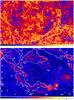 |
Fig. 6 |∇P|/|P| morphologies of the old SNRs Antlia (top) and G 353-34 (bottom) shown together with the contours of the Hα intensity from the all-sky map of Finkbeiner (2003). The units of contours for Antlia and G 353-34 are 0.1, 20, 40, 80, 160 and 0.1, 1.5, 8, 16, 32 Rayleigh, respectively. Intensity scale runs from 0.2 (black) to 2000 (white) and from 0.2 (black) to 1000 (white) for Antlia and G 353-34, respectively. |
3.3.3. |∇RM| features A, B, C
We note the presence in the |∇P|/|P| map (see labels A, B, C in Fig. 1) of three structures with no corresponding radio continuum emission. An elongated bubble-like feature (labelled A) is depicted at (l,b) ≈ (6°, −29°) with a linear size of about 2°. |∇P|/|P| and Hα intensity correlate, but the Hα intensity peaks at (l,b) ≈ (8°, −30°). A high normalized polarization gradient filament is seen across the feature and displays a single-jump morphology as shown in Fig. 7.
A long (~8.4 deg) and thick (~0.9 deg) linear structure (labelled B) extends from (l,b) ≈ (346°.6, −14°.8) to (l,b) ≈ (339°.3, −17°.1), and is prominent in both the |∇P|/|P| and Hα maps, as displayed in Fig. 7. The morphology of the |∇P|/|P| intensity may consist of two-filaments, both showing a single-jump morphology and slightly diverging towards (l,b) ≈ (339°.3, −17°.1), or a single filament displaying a double-jump morphology. The comparison with the simulated maps favours the two filaments case. The mean width of the upper and lower filaments is about 14′and 21′, respectively. The |∇P|/|P| intensity correlates with Hα, which shows a peak of ~12 Rayleigh (1 Rayleigh = 106/4π photons cm-2 s-1 sr-1) at (l,b) ≈ (343°.0, −16°.0). The Hα contrast of the structure with respect the background is ~2 around the peak position, decreasing to ~1.3 over the rest of the feature. The mean Hα contrast corresponds to an emission measure (EM) of about 4.4 pc cm-6. The polarization horizon of the |P| map places an upper limit of about 3 kpc on the distance, implying a length of ≲440 pc, a width of ≲50 pc, and a height of ≲900 pc above the Galactic plane. Such extended structures are observed in numerical simulations with sub-Alfvénic magnetic field strengths (see Burkhart et al. 2012). Linear features may be organized by large-scale magnetic fields and observed perpendicular to the field orientation.
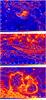 |
Fig. 7 |∇P|/|P| morphologies of the |∇RM| features labelled A, B, and C in Fig. 1 shown together with the contours of the Hα intensity from the all-sky map of Finkbeiner (2003). The units of the Hα contours for feature A (top panel), B (middle panel) and C (bottom panel) are 0.1, 2, 3, 4, 16 and 3, 4, 7, 16, 50 and 3, 5, 8, 16, 32 Rayleigh, respectively. Colour scale is the same as in Fig. 2. |
Finally, two prominent shell-like features are seen in |∇P|/|P| towards the third Galactic quadrant. The loops are not symmetric, are characterized by high normalized polarization gradients and have centres at (l,b) ≈ (251°,20°) and (l,b) ≈ (242°.5,17°.5), with radii of about 3° and 2°, respectively. Along with the extended filaments tracing the edges, a mottled pattern of high |∇P|/|P| intensity is also seen on small (≲0.5°) scales. No correlation with Hα intensity is found for these structures or their surroundings, thus disfavouring the presence of a relevant enhancement of the electron density due to an, e.g., H ii region. Moreover, the |∇P|/|P| filaments are characterized by a single-jump morphological pattern, suggesting the presence of a cusp or shear in the medium.
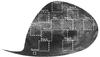 |
Fig. 8 Selected boxed regions of the |∇P|/|P| map for the statistical determination of the sonic Mach number. |
4. ISM turbulent regimes
Polarization gradients are useful means to study turbulence and to constrain the Mach numbers of diffuse and ionized gas because they are sensitive to variations in the free electron density and magnetic field strength. Variations in both the free electron density and magnetic field strength can be induced by strong shocks, thus polarization gradients are effective tracers of transonic and supersonic type turbulence. In addition, turbulence naturally induces discontinuities even in the incompressible limit, so polarization gradients can also indicate subsonic regimes.
The statistical determination of the sonic Mach number is possible because of the relationship between turbulence regimes and the probability distribution functions (PDFs) of the image intensity distribution (Burkhart et al. 2012). The probability distribution function of an image distribution gives the frequency of occurrence of intensities values and can be described by the main statistical moments: mean, variance, skewness, and kurtosis. The higher order moments (skewness and kurtosis) measure the degree of deviation of the PDF from a Gaussian, and are sensitive to the imprints of turbulence encoded in the image intensity distribution. For this reason, their use constitutes a common diagnostic for astrophysical turbulence.
The first-and second-order statistical moments (mean and variance) used here are defined as
follows:  and
and  , respectively,
with N the total number of elements and ξi the distribution of
intensities. The third and fourth order moments, skewness, and kurtosis, respectively, are
defined as
, respectively,
with N the total number of elements and ξi the distribution of
intensities. The third and fourth order moments, skewness, and kurtosis, respectively, are
defined as  where
where
 is the standard deviation. In this section, we investigate whether there is any large-scale
spatial dependence of the ISM turbulence regime as seen in the |∇P|/|P| map. To search for spatial
variations of the interstellar sonic Mach number, we selected eleven 25° × 25° sub-fields in
the |∇P|/|P| map, as shown in
Fig. 8. These regions cover the relevant extended
features seen in the map of spatial gradient of linear polarization, and sample a wide range
of Galactic longitude and latitude. A small test region showing no extended emission was
also chosen to characterize the noise statistics.
is the standard deviation. In this section, we investigate whether there is any large-scale
spatial dependence of the ISM turbulence regime as seen in the |∇P|/|P| map. To search for spatial
variations of the interstellar sonic Mach number, we selected eleven 25° × 25° sub-fields in
the |∇P|/|P| map, as shown in
Fig. 8. These regions cover the relevant extended
features seen in the map of spatial gradient of linear polarization, and sample a wide range
of Galactic longitude and latitude. A small test region showing no extended emission was
also chosen to characterize the noise statistics.
We show correlations between the first-and second-order moments of |∇P|/|P| of the twelve selected regions in the top panel of Fig. 9, and the correlation between the third-and fourth-order moments in the bottom panel of Fig. 9. Tight correlations exist for the moments of all twelve maps, and interesting trends are seen with respect to Galactic latitude and level of noise. In general the noise maps have very low values for all four moments, and the low values of the higher order moments indicate that the noise is Gaussian in nature. Regions with more structure exhibit higher values of the four moments, hence departures from Gaussianity. In all fields towards the plane, the values of the moments are very high, while the off-plane regions show a range of moments, which may indicate systematic variations in the ISM turbulence regime.
Figure 9 shows the moments for the S-PASS |∇P|/|P| data. However if we would like to compare the S-PASS moments with ideal MHD simulations, we must keep in mind two limitations of the observational data and simulated observations. First, the simulations cannot be normalized by the linear polarization map because they contain only “Faraday thin” structures (i.e. the emission and Faraday rotation take places in spatially separated regions) and have no intrinsic background polarization fluctuations. Thus as in the case of the ideal synthetic observations used by Gaensler et al. (2011), one must work with the statistics of the |∇P| map alone. Second, the observed polarization gradient fluctuations can only be interpreted in terms of turbulence once one has confirmed that the polarization signal is due to foreground Faraday rotation. In this scenario, there should be little correlation between the fluctuations of |P| and Stokes I. In the case where P or |∇P| or |∇P|/|P| matches the morphology seen in Stokes I, the polarized emission has a substantial intrinsic component and therefore does not necessarily describe the foreground turbulence along the line of sight.
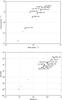 |
Fig. 9 Mean vs. variance (top) and skewness vs. kurtosis (bottom) for selected regions of the |∇P|/|P| map. Noise-dominated regions are indicated by crosses, the X symbol referring to the noise test region. Regions close to and off the Galactic plane are marked by filled squares and points, respectively. |
Main properties of the selected regions and their correlation degree of |P| with Stokes I (Col. 3), as derived by the Pearson’s coefficient (ρp) which assumes a linear relationship.
We show the Pearson correlation coefficients of |P| with Stokes I in Table 3 for each region. The Pearson coefficient measures the linearity of a relationship, while the Spearman’s rank coefficient measures any correlation. We tested it because the linear relationship between Stokes I and |P| is expected in the Faraday thin approximation. We see that in general strong correlations do not exist between |P| with Stokes I in these maps.
Since there is no strong correlation between |P| and Stokes I, we can assume that the bulk of the emission and features seen in |∇P|/|P| arise from (foreground) Faraday fluctuations in the turbulent MIM. Moreover, for cases that are properly described by the Faraday thin approximation, |∇P|/|P| will tend to |∇P| and the quantitative comparison with simulations is meaningful. Thus we can make a comparison between the statistics of |∇P| of the S-PASS observations and the MHD turbulence simulations of Burkhart et al. (2012), since the emission in both arises from turbulent fluctuations of ne and B along the line of sight. This is the aim of the next section.
4.1. Moments of |∇P| and the sonic Mach number
To test the goodness of the “Faraday thin” approximation for the selected regions, we
look at the correlation degree between |P| and |∇P|/|P|. To this aim we use both the
Pearson and the Spearman rank (ρs) correlation coefficients, with
ρs defined as
 (7)with
di the difference in
paired ranks of |P| and |∇P|/|P| intensities. As discussed in
Sect. 2.1, a negligible correlation is expected
between |P| and |∇P|/|P| in the Faraday thin regime with no
intrinsic background polarization fluctuations. However, intrinsic background polarization
fluctuations affect our data, so we assume |ρ|< 0.5 as a threshold for
low or mild correlation.
(7)with
di the difference in
paired ranks of |P| and |∇P|/|P| intensities. As discussed in
Sect. 2.1, a negligible correlation is expected
between |P| and |∇P|/|P| in the Faraday thin regime with no
intrinsic background polarization fluctuations. However, intrinsic background polarization
fluctuations affect our data, so we assume |ρ|< 0.5 as a threshold for
low or mild correlation.
Summary of high-order moments analysis obtained from selected “Faraday thin” regions.
The relationship between Pearson and Spearman’s rank correlation coefficients of |P| and |∇P|/|P| for each region is displayed in Table 3. In general, ρp and ρs point to the same results only in the following (extreme) cases: a linear relationship exists between the inspected variables, or the variables are uncorrelated. A sample of seven regions is selected: two are noise-dominated and two or three fields lie towards to/off the Galactic plane, respectively. The noise (dominated) regions display the lowest degree of correlation for both the correlation coefficients. For each selected region, we check the degree of correlation between |∇P| and |∇P|/|P| maps, finding mild or high values (i.e. >0.5) of the Spearman’s rank correlation coefficient. We then assume the Faraday thin approximation to hold for these few regions that sample a wide range of Galactic longitude and latitude. The small test region showing no extended emission is included to characterize the noise statistics. To search for spatial variations of the interstellar sonic and number, results from the statistical analysis of signal distributions of boxed 25° × 25° sized sub-fields in the |∇P| map are then matched with numerical simulations of isothermal compressible MHD turbulence, since the emission in both arises from turbulent fluctuations of ne and B along the line of sight.
Following Burkhart et al. (2012), we performed a statistical determination of the sonic Mach number by using the probability distribution function moments of the image distribution. In the framework of polarization gradients, the relationship between the moments of the |∇P| map and the sonic Mach number has been studied by Burkhart et al. (2012). As a consequence of the shock fronts creating more discontinuities and sharper gradients, a systematic increase in all four moments with increasing sonic Mach number is found.
In the analysis that follows, we employ the same set of MHD simulations that was used in the study by Burkhart et al. (2012) to estimate the sonic Mach number in S-PASS data. The database of 3D numerical simulations of isothermal compressible (MHD) turbulence is generated by using the MHD code of Cho & Lazarian (2003) and varying the input values for the sonic and Alfvénic Mach number. We scale the simulations to physical units, adopting typical parameters for warm ionized gas. We assume an average density of 0.1 cm-3 (Gaensler et al. 2011). The simulations are assumed to be fully ionized, and we do not include the effects of partial ionization. To make the maps of |∇P|, we first calculate the line of sight rotation measure at each pixel, then take the gradient of this rotation measure map and convert it to |∇P|. For more information and details on these simulations, we refer the reader to Cho & Lazarian (2003) and Burkhart et al. (2012).
An additional effect that must be considered when applying the moments to estimate the sonic Mach number in |∇P| data is the question of the telescope resolution. It is clear from the analysis of Burkhart et al. (2012) that smoothing changes the distribution of maps of |∇P|. As the resolution of maps of Stokes Q and U decreases, so do the moments. Thus one needs to take the smoothing of the data into account when comparing PDFs of |∇P|. We address this issue in the current study by applying four-pixel smoothing (equivalent to 10.75′ smoothing assuming that a scaling of one of our pixels at 512 × 512 resolution is 0.048 degrees) to the simulated |∇P| maps. This conversion is appropriate because the actual beam size of interest is a combination of the size scale of the beam in relation to the size scale of the turbulent injection. Given that the S-PASS maps we investigate are 25 × 25 degrees wide with a polarization horizon of ≈3 kpc, this means we are sampling emission in these boxes up to scales of ≈1 kpc. This is larger than the scale of the injection of turbulence in the Galaxy, but compatible with the large-scale driving of turbulence in our simulations.
4.1.1. Moments analysis: results
We calculated the values of the first four statistical moments of the sub-field regions of the S-PASS selected Faraday thin regions and compared the values with what is found in MHD simulations for different values of the sonic Mach number (see Burkhart et al. 2012). We used the full 512 × 512 sub-fields for calculating of the skewness and kurtosis in order to obtain meaningful estimates (Dudok de Wit 2004). However, simulations show that this condition might be relaxed somewhat, while still retaining valid results (Burkhart et al. 2010). Table 4 lists the results of calculating the moments for the S-PASS regions. Columns 3–6 show the all-map values of the skewness and kurtosis. We compare these values with the findings of Burkhart et al. (2012), who report values of skewness and kurtosis for sonic Mach numbers ranging from subsonic to supersonic values of upwards of 10. Subsonic cases have typical values of skewness ≲1.6 and values of kurtosis ≲5. Transonic simulations show values of skewness from 1.6–3 and kurtosis values from 5–17. Values higher than these are generally in the range of supersonic turbulence.
From the values presented in Table 4, a tight correlation can be found between mean and variance and between skewness and kurtosis, with the highest sonic Mach numbers corresponding to the highest values of moments and the lowest corresponding to low Mach numbers. We find this correlation behaviour of the four main moments also in the simulations, regardless of the addition of beam smoothing. Noise-dominated regions show systematically low values of the mean, the variance, and to a lesser extent, the skewness and kurtosis. In order to highlight any spatial dependence of the higher order moments for the selected regions in our data, we plot the calculated all-map skewness and kurtosis as a function of Galactic coordinates in Fig. 10. A clear correlation of both skewness and kurtosis as a function of Galactic latitude is seen, with the mid Galactic latitude regions showing slightly higher skewness and kurtosis. However, this trend implies only a weak variation in the sonic Mach number. As a consequence, no systematic clustering of the sonic Mach number values as a function of Galactic latitude is found, as is seen in the lower panel of Fig. 10.
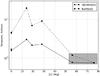 |
Fig. 10 Skewness and kurtosis as a function of Galactic latitude for the “Faraday thin” selected regions of the |∇P| map. Noise-dominated regions are indicated by the shaded box. |
5. Discussion
Figure 3 shows that the distribution peak position of the |∇P|/|P| intensities at Galactic latitudes |b|< 15° differs systematically from the peak positions at higher latitude ranges. The evident shift towards lower intensity values for higher Galactic latitudes observed towards the inner regions relates to the vertical extension of the Carina-Sagittarius spiral arm. Assuming a distance of ~2 kpc to this arm, the corresponding height above the Galactic disk is ≲500 pc, in agreement with the typical vertical extension of other arms (Feitzinger & Spicker 1986) and the scale height of the arms in the Taylor & Cordes (1993) model of the free electron density.
Moreover, the |∇P|/|P| intensity shows a dependence on both Galactic longitude and latitude. In Fig. 3 we find that |∇P|/|P| emission is roughly approximated by a log-normal distribution, with deviations towards small |∇P|/|P| fluctuations. A log-normal distribution is expected for pure density perturbations in a 3D turbulent and isothermal flow (see e.g. Vázquez-Semadeni 1994) and is observed for density tracers in the WIM such as the emission measure (Hill et al. 2008). However, our observations trace an additional part of the MIM, called the warm partially ionized medium (WPIM, see Heiles et al. 2001; Heiles & Haverkorn 2012). This component is colder than the WIM (T ≈ 5000 K) and does not emit Hα emission. However, it does contribute to the Faraday rotation in the medium. Therefore, our study traces both the WIM and WPIM, as opposed to the Hill et al. (2008) results that are only sensitive to the WIM. Furthermore the presence of magnetic fields in the MIM also influences the PDF of the perturbations (Kowal et al. 2007; Molina et al. 2012; Burkhart & Lazarian 2012b). Therefore, the deviations from a log-normal distribution we point out in Sect. 3.2 may be explained by the sensitivity of the |∇P|/|P| emission to both density and magnetic fluctuations. In addition, the presence in our data of a polarization horizon at a distance of about 3 kpc also affects the observed PDF of |∇P|/|P|. As a consequence, most of the diffuse polarized emission seen in the |∇P|/|P| map in Fig. 1 is generated within the nearest spiral arm. The short path length limits the number of the observed independent fluctuations, thus affecting the convergence to a Gaussian.
In Fig. 10 small variations of the sonic Mach number are observed in the Faraday-thin selected fields towards and out of the Galactic plane at medium latitudes. These variations may be consistent with turbulence in the MIM being driven by supernova explosions (see simulations by Hill et al. 2012), but they may also be explained by the presence of spatially extended and nearby objects triggering turbulence in (and interacting with) the surrounding medium. These features affect the statistical inference of the turbulent regime in some of the target regions. Since it is not possible to separate their contribution from the bulk of the |∇P| features, they were not masked.
Finally, we report the detection of a prominent spur-like feature (see Sect. 3) clearly seen towards the edge of the third Galactic quadrant in the |∇P|/|P| map but not traced by Hα intensity. Because of the high latitude, extinction is not likely to be responsible for the Hα non-detection, thus disfavouring a thermal electron density enhancement. Moreover, this magnetic structure has no radio continuum counterpart, suggesting that the direction of the magnetic field is mainly pointed towards the observer. The large angular size of this magnetic feature, which is specific of to the |∇P|/|P| map, suggests the structure is nearby. These characteristics, along with its shape, support its association with Loop I, a local feature of the ISM (Berkhuijsen et al. 1971; Heiles 1979) associated with an expanding SNR (Spoelstra 1972; Heiles 1998; Wolleben 2007).
6. Summary and conclusions
Normalized spatial gradients of the polarization vectors have been used for the first time to map the entire southern sky. The large sky coverage allows the exploration of cases not treated by the previous studies of Gaensler et al. (2011) and Burkhart et al. (2012). The S-PASS |∇P|/|P| map displays a wealth of filamentary structures with typical widths down to the angular resolution. The emission is characterized by a polarization horizon of about 3 kpc, implying density and magnetic fluctuations down to a linear scale <10 pc given the angular size of the S-PASS beam. An extended and patchy pattern of |∇P|/|P| intensity is found within the third and fourth Galactic quadrants at high (b ≲ −60°) latitudes towards the south Galactic pole.
Two different morphologies (i.e. “single” or “double” jump profiles) corresponding to different MHD turbulence cases (i.e. low or high sonic Mach numbers) are observed, thus supporting the predictions of numerical simulations (Burkhart et al. 2012). Normalized spatial gradients of the polarization vector are effective tracers of extended and Faraday rotating features, such as H ii regions and evolved SNRs. Indeed we clearly recognize the two known nearby and old SNRs Antlia and G 353-34. In addition, by combining the information from both the |∇P|/|P| and Hα intensity maps we can highlight the presence of both electron density and magnetic structures, in agreement with simulations (Burkhart et al. 2012).
Although multiple scales of energy injection are expected in the ISM (Nota & Katgert 2010), instabilities triggered by supernova events and Galactic shear in the ISM are expected to mainly generate and sustain interstellar MHD turbulence (Mac Low 2004; Hill et al. 2012). Observational studies of turbulence in the warm and ionized ISM also indicate a spectral index matching that of the Goldreich & Sridhar (1995) theory of Alfvénic turbulence, consistent with a weakly compressible medium. This is the case for transonic turbulence as shown by Hill et al. (2008), who estimated the sonic Mach number by comparing statistics of Hα WHAM data with simulations. By applying a moment analysis to a number of fields, we extend it to the MIM and confirm the earlier result of these authors, finding lines of sight to be consistent with Ms ≲ 2 (see Table 4).
The use of the spatial gradient of linear polarizations combined with a robust statistical analysis makes mapping of the sonic and Alfvénic Mach numbers spatial variations in the MIM a feasible and mandatory aim of forthcoming radio observations at high angular resolution. These studies will allow us to gain complementary insight into the turbulence and shocks in the ionized ISM over a wide range of plasma β-parameter regimes. To gain a complete picture of Mach numbers and spatial variations in the MIM, complete sky coverage is needed, requiring a corresponding high resolution and sensitivity survey of the northern sky.
The catalogue is available at http://www.mrao.cam.ac.uk/surveys/snrs/
Acknowledgments
The authors thank the referee, Steven Spangler, for providing detailed comments and helpful suggestions in the preparation of the final manuscript. This work has been carried out in the framework of the S-band Polarisation All Sky Survey collaboration (S-PASS). The Parkes Radio Telescope is part of the Australia Telescope National Facility, which is funded by the Commonwealth of Australia for operation as a National Facility managed by CSIRO. The research leading to these results has received funding from the European Union’s Seventh Framework Programme (FP7/2007-2013) under grant agreement number 239490. This work is part of the research programme 639.042.915, which is (partly) financed by the Netherlands Organization for Scientific Research (NWO). Support for B.B. and A.L. comes from the NSF grant AST 1212096, and the Center for Magnetic Self-Organization in Laboratory and Astrophysical Plasmas (CMSO). B.B. acknowledges Vilas Associate Awards and the hospitality of the International Institute of Physics (Natal). Parts of this research were conducted by the Australian Research Council Centre of Excellence for All-sky Astrophysics (CAASTRO), through project number CE110001020. B.M.G. acknowledges support from the Australian Research Council through an Australian Laureate Fellowship (FL100100114).
References
- Armstrong, J. W., Rickett, B. J., & Spangler, S. R. 1995, ApJ, 443, 209 [NASA ADS] [CrossRef] [Google Scholar]
- Berdyugin, A., Piirola, V., & Teerikorpi, P. 2004, A&A, 424, 873 [NASA ADS] [CrossRef] [EDP Sciences] [Google Scholar]
- Berkhuijsen, E. M., Haslam, C. G. T., & Salter, C. J. 1971, A&A, 14, 252 [NASA ADS] [Google Scholar]
- Beuermann, K., Kanbach, G., & Berkhuijsen, E. M. 1985, A&A, 153, 17 [NASA ADS] [Google Scholar]
- Boulares, A., & Cox, D. P. 1990, ApJ, 365, 544 [NASA ADS] [CrossRef] [Google Scholar]
- Burkhart, B., & Lazarian, A. 2012a, Astrophysical MHD turbulence: confluence of observations, simulations, and theory. Proceedings of the International Astronomical Union, 8, 325 [Google Scholar]
- Burkhart, B., & Lazarian, A. 2012b, ApJ, 755, 19 [Google Scholar]
- Burkhart, B., Stanimirović, S.,Lazarian, A., & Kowal, G. 2010, ApJ, 708, 120 [Google Scholar]
- Burkhart, B., Lazarian, A., & Gaensler, B. M. 2012, ApJ, 749, 145 [NASA ADS] [CrossRef] [Google Scholar]
- Carretti, E., Haverkorn, M., McConnell, D., et al. 2009, Rev. Mex. Astron. Astrofis., 36, 9 [Google Scholar]
- Carretti, E., Crocker, R. M., Staveley-Smith, L., et al. 2013, Nature, 493, 66 [NASA ADS] [CrossRef] [PubMed] [Google Scholar]
- Chepurnov, A., & Lazarian, A. 2010, ApJ, 710, 853 [NASA ADS] [CrossRef] [Google Scholar]
- Chepurnov, A., Lazarian, A., Stanimirović, S., Heiles, C., & Peek, J. E. G. 2010, ApJ, 714, 1398 [NASA ADS] [CrossRef] [Google Scholar]
- Cho, J., & Lazarian, A. 2003, MNRAS, 345, 325 [NASA ADS] [CrossRef] [Google Scholar]
- Cox, D. A. 2005, ARA&A, 43, 337 [NASA ADS] [CrossRef] [EDP Sciences] [MathSciNet] [Google Scholar]
- Dodson, R., Legge, D., Reynolds, J. E., & McCulloch, P. M. 2003, ApJ, 596, 1137 [NASA ADS] [CrossRef] [Google Scholar]
- Dudok de Wit, T. 2004, Phys. Rev. E, 70, 5302 [CrossRef] [Google Scholar]
- Duncan, A. R., Stewart, R. T., Haynes, R. F., & Jones, K. L. 1995, MNRAS, 277, 36 [NASA ADS] [Google Scholar]
- Duncan, A. R., Haynes, R. F., Jones, K. L., & Stewart, R. T. 1997, MNRAS, 297, 279 [NASA ADS] [CrossRef] [Google Scholar]
- Elmegreen, B. G., & Scalo, J. 2004, ARA&A, 42, 211 [NASA ADS] [CrossRef] [Google Scholar]
- Feitzinger, J. V., & Spicker, J. 1986, PASJ, 38, 485 [NASA ADS] [Google Scholar]
- Ferrière, K. M. 2001, Rev. Mod. Phys., 73, 1031 [NASA ADS] [CrossRef] [Google Scholar]
- Finkbeiner, D. P. 2003, ApJS, 146, 407 [NASA ADS] [CrossRef] [Google Scholar]
- Gaensler, B. M., Dickey, J. M., McClure-Griffiths, N. M., et al. 2001, ApJ, 549, 959 [NASA ADS] [CrossRef] [Google Scholar]
- Gaensler, B. M., Madsen, G. J., Chatterjee, S., & Mao, S. A. 2008, PASA, 25, 184 [NASA ADS] [CrossRef] [Google Scholar]
- Gaensler, B. M., Haverkorn, M., Burkhart, B., et al. 2011, Nature, 478, 214 [NASA ADS] [CrossRef] [Google Scholar]
- Georgelin, Y. M., Russeil, D., Amram, P., et al. 2000, A&A, 357, 308 [NASA ADS] [Google Scholar]
- Ghavamian, P., Winkler, P. F., Raymond, J. C., & Long, K. S. 2002, ApJ, 572, 888 [NASA ADS] [CrossRef] [Google Scholar]
- Giacani, E. B., Dubner, G. M., Green, A. J., Goss, W. M., & Gaensler, B. M. 2000, AJ, 119, 281 [NASA ADS] [CrossRef] [Google Scholar]
- Goldreich, P., & Sridhar, S. 1995, ApJ, 438, 763 [NASA ADS] [CrossRef] [Google Scholar]
- Green, D. A. 2009, Bulletin of the Astronomical Society of India, 37, 45 [Google Scholar]
- Haslam, C. G. T., Klein, U., Salter, C. J., et al. 1981, A&A, 100, 209 [NASA ADS] [Google Scholar]
- Haverkorn, M., Gaensler, B. M., McClure-Griffiths, N. M., Dickey, J. M., & Green, A. J. 2004a, ApJ, 609, 776 [NASA ADS] [CrossRef] [Google Scholar]
- Haverkorn, M., Katgert, P., & de Bruyn, A. G. 2004b, A&A, 427, 169 [NASA ADS] [CrossRef] [EDP Sciences] [Google Scholar]
- Haverkorn, M., Brown, J. C., Gaensler, B. M., & McClure-Griffiths, N. M. 2008, ApJ, 680, 362 [NASA ADS] [CrossRef] [Google Scholar]
- Heiles, C. 1979, ApJ, 229, 533 [NASA ADS] [CrossRef] [Google Scholar]
- Heiles, C. 1998, in The Local Bubble and Beyond, eds. D. Breitschwerdt, M. J. Freyberg, & J. Truemper, IAU Colloq. 166, Lect. Notes in Phys. 506, 229 [Google Scholar]
- Heiles, C. 2001, in Tetons 4: Galactic Structure, Stars and the Interstellar Medium, eds. C. E. Woodward, M. D. Bicay, & J. M. Shull, ASP Conf. Ser., 231, 294 [Google Scholar]
- Heiles, C., & Haverkorn, M. 2012, Space Sci. Rev., 166, 293 [NASA ADS] [CrossRef] [EDP Sciences] [Google Scholar]
- Hill, A. S., Benjamin, R. A., Kowal, G., et al. 2008, ApJ, 686, 363 [NASA ADS] [CrossRef] [Google Scholar]
- Hill, A. S., Joung, M. R., Mac Low, M.-M., et al. 2012, ApJ, 750, 104 [NASA ADS] [CrossRef] [Google Scholar]
- Hinshaw, G., Weiland, J. L., Hill, R. S., et al. 2009, ApJS, 180, 225 [NASA ADS] [CrossRef] [Google Scholar]
- Hobbs, G., Lorimer, D. R., Lyne, A. G., & Kramer, M. 2005, MNRAS, 360, 974 [NASA ADS] [CrossRef] [Google Scholar]
- Iacobelli, M., Haverkorn, M., Orru, E., et al. 2013, A&A, 558, A72 [NASA ADS] [CrossRef] [EDP Sciences] [Google Scholar]
- Jonas, J. L., de Jager, G., & Baart, E. E. 1985, A&AS, 62, 105 [NASA ADS] [Google Scholar]
- Jonas, J. L., Baart, E. E., & Nicolson, G. D. 1998, MNRAS, 297, 977 [NASA ADS] [CrossRef] [Google Scholar]
- Kowal, G., Lazarian, A., & Beresnyak, A. 2007 ApJ, 658, 423 [NASA ADS] [CrossRef] [Google Scholar]
- Kobayashi, T., Komori, Y., Yoshida, K., & Nishimura, J. 2004, ApJ, 601, 340 [NASA ADS] [CrossRef] [Google Scholar]
- Krumholz, M. R., & McKee, C. F. 2005, ApJ, 630, 250 [NASA ADS] [CrossRef] [Google Scholar]
- Landecker, T. L., Uyaniker, B., & Kothes, R. 2002, in Astrophysical Polarized Backgrounds, eds. S. Cecchini, S. Cortiglioni, R. Sault, & C. Sbarra, AIP Conf. Proc., 609, 9 [Google Scholar]
- Lazarian, A., & Pogosyan, D. 2012, ApJ, 747, 5 [NASA ADS] [CrossRef] [Google Scholar]
- Lazarian, A., & Vishniac, E. T. 1999, ApJ, 517, 700 [NASA ADS] [CrossRef] [Google Scholar]
- Lazarian, A., Kowal, G., Vishniac, E., & de Gouveia Dal Pino, E. 2011, Planet. Space Sci., 59, 537 [NASA ADS] [CrossRef] [Google Scholar]
- Mac Low, M.-M. 2004, Ap&SS, 289, 323 [NASA ADS] [CrossRef] [Google Scholar]
- Manchester, R. N., Hobbs, G. B., Teoh, A., & Hobbs, M. 2005, AJ, 129, 1993 [NASA ADS] [CrossRef] [Google Scholar]
- McCullough, P. R., Fields, B. D., & Pavlidou, V. 2002, ApJ, 576, 41 [Google Scholar]
- McKee, C. F., & Ostriker, E. C. 2007, ARA&A, 45, 565 [NASA ADS] [CrossRef] [Google Scholar]
- Milne, D. K. 1970, Aust. J. Phys., 23, 425 [NASA ADS] [Google Scholar]
- Minter, A. H., & Spangler, S. R. 1996, ApJ, 458, 194 [NASA ADS] [CrossRef] [Google Scholar]
- Molina, F. Z., Glover, S. C. O., Federrath, C., & Klessen, R. S. 2012, MNRAS, 423, 628 [Google Scholar]
- Nota, T., & Katgert, P. 2010, A&A, 513, A65 [NASA ADS] [CrossRef] [EDP Sciences] [Google Scholar]
- Pogosyan, D., & Lazarian, A. 2009, Rev. Mex. Astron. Astrofis., 36, 54 [Google Scholar]
- Reich, P., Testori, J. C., & Reich, W. 2001, A&A, 376, 861 [NASA ADS] [CrossRef] [EDP Sciences] [Google Scholar]
- Sajina, A., Partridge, B., Evans, T., et al. 2011, ApJ, 732, 45 [NASA ADS] [CrossRef] [Google Scholar]
- Schlickeiser, R. 2011, ApJ, 732, 96 [NASA ADS] [CrossRef] [Google Scholar]
- Schnitzeler, D. H. F. M. 2012, MNRAS, 427, 664 [NASA ADS] [CrossRef] [Google Scholar]
- Schnitzeler, D. H. F. M., Katgert, P., & de Bruyn, A. G. 2007, A&A, 471, 21 [Google Scholar]
- Schnitzeler, D. H. F. M., Katgert, P., & de Bruyn, A. G. 2009, A&A, 494, 611 [NASA ADS] [CrossRef] [EDP Sciences] [Google Scholar]
- Spangler, S. 1982, ApJ, 261, 310 [NASA ADS] [CrossRef] [Google Scholar]
- Spangler, S. 1983, ApJ, 271, 49 [Google Scholar]
- Spoelstra, T. A. T. 1972, A&A, 21, 61 [NASA ADS] [Google Scholar]
- Taylor, J. H., & Cordes, J. M. 1993, ApJ, 411, 674 [NASA ADS] [CrossRef] [Google Scholar]
- Testori, J. C., Reich, P., & Reich, W. 2008, A&A, 484, 733 [NASA ADS] [CrossRef] [EDP Sciences] [Google Scholar]
- Tucci, M., Martínez-Gonzalez, E., Toffolatti, L., González-Nuevo, J., & De Zotti, G. 2004, MNRAS, 349, 1267 [NASA ADS] [CrossRef] [Google Scholar]
- Uyaniker, B., Landecker, T. L., Gray, A. D., & Kothes, R. 2003, ApJ, 585, 785 [NASA ADS] [CrossRef] [Google Scholar]
- Vallée, J. P. 2008, AJ, 135, 1301 [NASA ADS] [CrossRef] [Google Scholar]
- Vázquez-Semadeni, E. 1994, ApJ, 423, 681 [NASA ADS] [CrossRef] [Google Scholar]
- Vinokur, M. 1965, Ann. Astrophys., 28, 412 [NASA ADS] [Google Scholar]
- Wardle, J. F. C., & Kronberg, P. P. 1974, ApJ, 194, 249 [NASA ADS] [CrossRef] [Google Scholar]
- Wieringa, M. H., de Bruyn, A. G., Jansen, D., Brouw, W. N., & Katgert, P. 1993, A&A, 268, 215 [NASA ADS] [Google Scholar]
- Wolleben, M. 2007, ApJ, 664, 349 [NASA ADS] [CrossRef] [Google Scholar]
All Tables
List of unambiguously identified SNRs in all of Stokes I, polarized intensity, and polarization gradient S-PASS maps, by cross-checking radio data taken from the Green (2009) database.
Main properties of the selected regions and their correlation degree of |P| with Stokes I (Col. 3), as derived by the Pearson’s coefficient (ρp) which assumes a linear relationship.
Summary of high-order moments analysis obtained from selected “Faraday thin” regions.
All Figures
|
Fig. 1 Map of the normalised spatial gradient of linearly polarized emission, |∇P|/|P|, in Aitoff projection of the entire southern sky at a reference frequency of 2.3 GHz and a resolution of 11′. The noise level in the map was obtained by averaging intensity over a small region with no signal and intensity is clipped at 3σ. The scaling runs from 0.2 (black) to 1000 (white). Intensity unit is beam-0.5. |
| In the text | |
|
Fig. 2 A zoom of Fig. 1 centred on l ~ 278°, b ~ 22°, showing different observed morphologies for different MHD turbulence cases “double-jumps” (D boxed region) and “single-jump” (S boxed region) filaments due to (strong or weak) shocks and a cusps or shears along the line of sight, respectively. Intensity scale runs from 0.2 (black) to 2000 (white). |
| In the text | |
|
Fig. 3 Distributions of the |∇P|/|P| intensity of the masked map at four ranges of Galactic latitude (|b|). Statistical errors in each intensity bin are also shown. |
| In the text | |
|
Fig. 4 Mean (solid lines) and standard (dashed lines) deviation profiles towards the Galactic disk (5° ≲|b|≲ 10°) for the |∇P|/|P| intensity as a function of Galactic longitude. The ranges of Galactic longitudes corresponding to the main Galactic features and spiral arms are also indicated. Data points are obtained from square regions of size 5°. |
| In the text | |
|
Fig. 5 Bubble-like |∇P|/|P| morphology of the nearby H ii regions Sh 2-27 (on the left) and Sh 2-7 (on the right) shown together with the contours of the Hα intensity from the all-sky map of Finkbeiner (2003). The units of contours are 1, 13, 25, 50 and 100 Rayleigh. Colour scale is the same as in Fig. 2. |
| In the text | |
|
Fig. 6 |∇P|/|P| morphologies of the old SNRs Antlia (top) and G 353-34 (bottom) shown together with the contours of the Hα intensity from the all-sky map of Finkbeiner (2003). The units of contours for Antlia and G 353-34 are 0.1, 20, 40, 80, 160 and 0.1, 1.5, 8, 16, 32 Rayleigh, respectively. Intensity scale runs from 0.2 (black) to 2000 (white) and from 0.2 (black) to 1000 (white) for Antlia and G 353-34, respectively. |
| In the text | |
|
Fig. 7 |∇P|/|P| morphologies of the |∇RM| features labelled A, B, and C in Fig. 1 shown together with the contours of the Hα intensity from the all-sky map of Finkbeiner (2003). The units of the Hα contours for feature A (top panel), B (middle panel) and C (bottom panel) are 0.1, 2, 3, 4, 16 and 3, 4, 7, 16, 50 and 3, 5, 8, 16, 32 Rayleigh, respectively. Colour scale is the same as in Fig. 2. |
| In the text | |
|
Fig. 8 Selected boxed regions of the |∇P|/|P| map for the statistical determination of the sonic Mach number. |
| In the text | |
|
Fig. 9 Mean vs. variance (top) and skewness vs. kurtosis (bottom) for selected regions of the |∇P|/|P| map. Noise-dominated regions are indicated by crosses, the X symbol referring to the noise test region. Regions close to and off the Galactic plane are marked by filled squares and points, respectively. |
| In the text | |
|
Fig. 10 Skewness and kurtosis as a function of Galactic latitude for the “Faraday thin” selected regions of the |∇P| map. Noise-dominated regions are indicated by the shaded box. |
| In the text | |
Current usage metrics show cumulative count of Article Views (full-text article views including HTML views, PDF and ePub downloads, according to the available data) and Abstracts Views on Vision4Press platform.
Data correspond to usage on the plateform after 2015. The current usage metrics is available 48-96 hours after online publication and is updated daily on week days.
Initial download of the metrics may take a while.