| Issue |
A&A
Volume 566, June 2014
|
|
|---|---|---|
| Article Number | A8 | |
| Number of page(s) | 16 | |
| Section | Numerical methods and codes | |
| DOI | https://doi.org/10.1051/0004-6361/201220021 | |
| Published online | 29 May 2014 | |
Probabilistic positional association of catalogs of astrophysical sources: the Aspects code ⋆,⋆⋆
Institut d’Astrophysique de Paris, UPMC – Univ. Paris 6, CNRS, UMR 7095, 98bis boulevard Arago, 75014 Paris, France
e-mail: Michel.Fioc@iap.fr
Received: 16 July 2012
Accepted: 1 November 2013
We describe a probabilistic method of cross-identifying astrophysical sources in two catalogs from their positions and positional uncertainties. The probability that an object is associated with a source from the other catalog, or that it has no counterpart, is derived under two exclusive assumptions: first, the classical case of several-to-one associations, and then the more realistic but more difficult problem of one-to-one associations. In either case, the likelihood of observing the objects in the two catalogs at their effective positions is computed and a maximum likelihood estimator of the fraction of sources with a counterpart – a quantity needed to compute the probabilities of association – is built. When the positional uncertainty in one or both catalogs is unknown, this method may be used to estimate its typical value and even to study its dependence on the size of objects. It may also be applied when the true centers of a source and of its counterpart at another wavelength do not coincide. To compute the likelihood and association probabilities under the different assumptions, we developed a Fortran 95 code called Aspects ([aspε], “Association positionnelle/probabiliste de catalogues de sources” in French); its source files are made freely available. To test Aspects, all-sky mock catalogs containing up to 105 objects were created, forcing either several-to-one or one-to-one associations. The analysis of these simulations confirms that, in both cases, the assumption with the highest likelihood is the right one and that estimators of unknown parameters built for the appropriate association model are reliable.
Key words: methods: statistical / catalogs / galaxies: statistics / stars: statistics / astrometry
Available at www2.iap.fr/users/fioc/Aspects/
The Aspects code is available at the CDS via anonymous ftp to cdsarc.u-strasbg.fr (130.79.128.5) or via http://cdsarc.u-strasbg.fr/viz-bin/qcat?J/A+A/566/A8
© ESO, 2014
1. Introduction
The most basic method of cross-identifying two catalogs K and K′ with known circular positional uncertainties is to consider that a K′-source M′ is the same as an object M of K if it falls within a disk centered on M and having a radius equal to a few times their combined positional uncertainty; if the disk is void, M has no counterpart, and if it contains several K′-sources, the nearest one is identified to M. This solution is defective for several reasons: it does not take the density of sources into account; positional uncertainty ellipses are not properly treated; the radius of the disk is arbitrary; positional uncertainties are not always known; K and K′ do not play symmetrical roles; the identification is ambiguous if a K′-source may be associated to several objects of K. Worst of all, it does not provide a probability of association.
Beyond this naïve method, the cross-identification problem has been studied by Condon et al. (1975), de Ruiter et al. (1977), Prestage & Peacock (1983), Sutherland & Saunders (1992), Bauer et al. (2000), and Rutledge et al. (2000), among others. As shown by the recent papers of Budavári & Szalay (2008), Brand et al. (2006), Rohde et al. (2006), Roseboom et al. (2009), and Pineau et al. (2011), this field is still very active and will be more so with the wealth of forthcoming multiwavelength data and the virtual observatory (Vignali et al. 2009). In these papers, the identification is performed using a “likelihood ratio”. For two objects (M,M′) ∈ K × K′ with known coordinates and positional uncertainties, and given the local surface density of K′-sources, this ratio is typically computed as 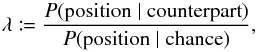 (1)where P(position | counterpart) is the probability of finding M′ at some position relative to M if M′ is a counterpart of M, and P(position | chance) is the probability that M′ is there by chance. As noticed by Sutherland & Saunders (1992), there has been some confusion when defining and interpreting λ, and, more importantly, in deriving the probability 1 that M and M′ are the same.
To associate sources from catalogs at different wavelengths, some authors include some a priori information on the spectral energy distribution (SED) of the objects in this likelihood ratio. When this work started, our primary goal was to build template observational SEDs from the optical to the far-infrared for different types of galaxies. We initially intended to cross-identify the Iras Faint Source Survey (Moshir et al. 1992, 1993) with the Leda database (Paturel et al. 1995). Because of the high positional inaccuracy of Iras data, special care was needed to identify optical sources with infrared ones. While Iras data are by now quite outdated and have been superseded by Spitzer and Herschel observations, we think that the procedure we began to develop at that time may be valuable for other studies. Because we aimed to fit synthetic SEDs to the template observational ones, we could not and did not want to make assumptions on the SED of objects based on their type, since this would have biased the procedure. We therefore rely only on positions in what follows.
The method we use is in essence similar to that of Sutherland & Saunders (1992). Because thinking in terms of probabilities rather than of likelihood ratios highlights some implicit assumptions, we found it however useful for the sake of clarity to detail hereafter our calculations. This allows us moreover to propose a systematic way to estimate the unknown parameters required to compute the probabilities of association and to extend our work to a case not covered by the papers cited above (see Sect. 4).
After some preliminaries (Sect. 2), we compute in Sect. 3 the probability of association under the hypothesis that a K-source has at most one counterpart in K′ but that several objects of K may share the same one (“several-to-one” associations). We also compute the likelihood to observe all the sources at their effective positions and use it to estimate the fraction of objects with a counterpart and, if unknown, the positional uncertainty in one or both catalogs. In Sect. 4, we do the same calculations under the assumption that a K-source has at most one counterpart in K′ and that no other object of K has the same counterpart (“one-to-one” associations). In Sect. 5, we present a code, Aspects, implementing the results of Sects. 3 and 4, and with which we compute the likelihoods and probabilities of association under the aforementioned assumptions. We test it on simulations in Sect. 6. The probability distribution of the relative positions of associated sources is modeled in Appendix A.
2. Preliminaries
2.1. Notations
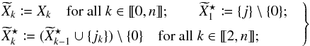
We consider two catalogs K and K′ defined on a common surface of the sky, of area S, and containing respectively n sources (Mi)i ∈ [[1,n]] and  sources
 ![\hbox{$(\Mp_j)^{}_{\smash[t]{j\in\integinterv{1}{\np}}}$}](/articles/aa/full_html/2014/06/aa20021-12/aa20021-12-eq16.png) . We define the following events:
. We define the following events:
-
ci: Mi is in the infinitesimal surface element d2ri located at ri;
-
 :
:  is in the infinitesimal surface element
  located at
  ;
; -
 : the coordinates of all K-sources are known;
 -
 : the coordinates of all K′-sources are known;
 -
Ai,j, with i ≠ 0 and j ≠ 0:
is a counterpart of Mi; -
Ai, 0: Mi has no counterpart in K′, i.e.
 , where
  is the negation of an event ω;
 -
A0,j:
has no counterpart in K.
We denote by f (resp. f′) the unknown a priori (i.e., not knowing the coordinates) probability that any element of K (resp. K′) has a counterpart in K′ (resp. K). In terms of the events (Ai,j), for any  ,
, 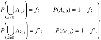 (2)We see in Sects. 3.2 and 4.2 how to estimate f and f′.
The angular distance between two points Y and Z is written ψ(Y,Z). More specifically, we put  .
.
2.2. Assumptions
Calculations are carried out under one of three exclusive assumptions:
-
Several-to-one hypothesis:
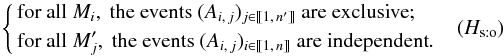 Therefore, a K-source has at most one counterpart in K′, but a K′-source may have several counterparts in K. Since more K-sources have a counterpart in K′ than the converse,
  . This assumption is reasonable if the angular resolution in K′ (e.g. Iras) is much poorer than in K (e.g. Leda), since several distinct objects of K may then be confused in K′.
 -
One-to-several hypothesis: the symmetric of assumption (Hs:o), i.e.,
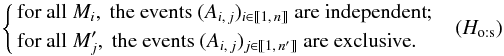 In that case,
  . This assumption is appropriate for catalogs of extended sources that, although observed as single at the wavelength of K, may look broken up at the wavelength of K′.
 -
One-to-one hypothesis: any K-source has at most one counterpart in K′ and reciprocally, i.e.
 Then,
Then,  . This assumption is the most relevant one for high-resolution catalogs of point sources or of well-defined extended sources.
Probabilities, likelihoods, and estimators specifically derived under either assumption (Hs:o), (Ho:s), or (Ho:o) are written with the subscript “s:o”, “o:s”, or “o:o”, respectively; the subscript “:o” is used for results valid for both (Hs:o) and (Ho:o). The “several-to-several” hypothesis where all the events  are independent is not considered here.
We make two other assumptions: all the associations Ai,j with i ≠ 0 and j ≠ 0 are considered a priori as equally likely, and the effect of clustering is negligible.
2.3. Approach
Our approach is the following. For each of the assumptions (Hs:o), (Ho:o), and (Ho:s), we
-
find an expression for the probabilities of association,
-
build estimators of the unknown parameters needed to compute these probabilities, and
-
compute the likelihood of the assumption from the data.
Then, we compute the probabilities of association for the best estimators of unknown parameters and the most likely assumption.
Although (Hs:o) is less symmetrical and neutral than (Ho:o), we begin our study with this assumption: first, because computations are much simpler under (Hs:o) than under (Ho:o) and serve as a guide for the latter; second, because they provide initial values for the iterative procedure (Sect. 5.4.3) used to effectively compute probabilities under (Ho:o).
3. Several-to-one associations
In this section, we assume that hypothesis (Hs:o) holds. As shown in Sect. 3.3, this is also the assumption implicitly made by the authors cited in the introduction.
3.1. Probability of association: global computation
We want to compute2 the probability P(Ai,j | C ∩ C′) of association between sources Mi and (j ≠ 0) or the probability that Mi has no counterpart (j = 0), knowing the coordinates of all the objects in K and K′. Remembering that, for any events ω1, ω2, and ω3, P(ω1 | ω2) = P(ω1 ∩ ω2) /P(ω2) and thus 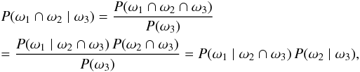 (3)we have, with ω1 = Ai,j, ω2 = C, and ω3 = C′,
 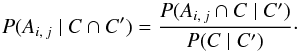 (4)
(4)
3.1.1. Computation of Ps:o(C | C′)
We first compute the denominator of Eq. (4)3. The event 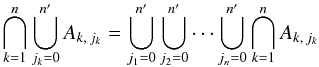 (5)is certain by definition of the Ak,jk and, under either assumption (Hs:o) or (Ho:o), Ak,ℓ ∩ Ak,m =? for all Mk if ℓ ≠ m. Consequently, using the symbol for mutually exclusive events instead of , we obtain
 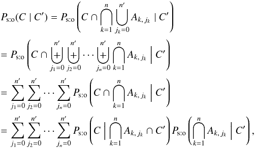 (6)with ω1 = C,
 ![\hbox{$\omega_2 = \bigcap_{\smash[t]{k=1}}^n A_{k\comma j_k}$}](/articles/aa/full_html/2014/06/aa20021-12/aa20021-12-eq77.png) , and ω3 = C′ in Eq. (3).
, and ω3 = C′ in Eq. (3).
Since ![\hbox{$C = \bigcap_{\smash[t]{k=1}}^n c_k$}](/articles/aa/full_html/2014/06/aa20021-12/aa20021-12-eq78.png) , the first factor in the product of Eq. (6)is
, the first factor in the product of Eq. (6)is 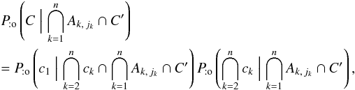 (7)with ω1 = c1,
 ![\hbox{$\omega_2 = \bigcap_{\smash[t]{k=2}}^n c_k$}](/articles/aa/full_html/2014/06/aa20021-12/aa20021-12-eq81.png) , and ω3 = Ak,jk ∩ C′ in Eq. (3). Doing the same with
, and ω3 = Ak,jk ∩ C′ in Eq. (3). Doing the same with ![\hbox{$\bigcap_{\smash[t]{k=2}}^n c_k$}](/articles/aa/full_html/2014/06/aa20021-12/aa20021-12-eq83.png) instead of C, we obtain
instead of C, we obtain 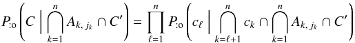 (8)by iteration.
If jℓ ≠ 0, Mℓ is only associated with  . Consequently,
 ![\begin{eqnarray} \Pato\Left(c_\ell \Bigm| \bigcap_{k=\ell+1}^n c_k \cap \bigcap_{k=1}^n A_{k\comma j_k} \cap C'\Right) &=& \Pato(c_\ell \mid A_{\ell\comma j_\ell} \cap c'_{\smash[t]{j_\ell}}) \notag \\ &=& \xi_{\ell\comma j_\ell} \multspace \df^2\vec r_\ell, \label{jl_non_nul} \end{eqnarray}](/articles/aa/full_html/2014/06/aa20021-12/aa20021-12-eq89.png) (9)where, denoting by
(9)where, denoting by ![\hbox{$\vec r_{\ell\comma j_\ell} \coloneqq \vec r'_{\smash[t]{j_\ell}} - \vec r_\ell$}](/articles/aa/full_html/2014/06/aa20021-12/aa20021-12-eq90.png) the position vector of relative to Mℓ and by Γℓ,jℓ the covariance matrix of rℓ,jℓ (cf. Appendix A.2),
the position vector of relative to Mℓ and by Γℓ,jℓ the covariance matrix of rℓ,jℓ (cf. Appendix A.2), ![\begin{equation} \xi_{\ell\comma j_\ell} = \frac{ \exp\left( -\frac{1}{2}\multspace \transpose{\vec r}_{\smash[t]{\ell\comma j_\ell}} \cdot \Gamma_{\smash[t]{\ell\comma j_\ell}}^{-1} \cdot \vec r_{\ell\comma j_\ell} \right) }{ 2\multspace \piup\multspace \!\sqrt{\det \Gamma_{\ell\comma j_\ell}} }\cdot \end{equation}](/articles/aa/full_html/2014/06/aa20021-12/aa20021-12-eq93.png) (10)If jℓ = 0, Mℓ is not associated with any source in K′. Since clustering is neglected,
(10)If jℓ = 0, Mℓ is not associated with any source in K′. Since clustering is neglected, ![\begin{equation} \Pato\left(c_\ell \Bigm| \bigcap_{k=\ell+1}^n c_k \cap \bigcap_{k=1}^\np c'_{\smash[t]{k}} \cap \bigcap_{k=1}^n A_{k\comma j_k}\right) = \Pato(c_\ell \mid A_{\ell\comma 0}) = \xi_{\ell\comma 0}\multspace \df^2\vec r_\ell, \label{jl_nul} \end{equation}](/articles/aa/full_html/2014/06/aa20021-12/aa20021-12-eq95.png) (11)where the last equality defines the spatial probability density ξℓ, 0; for the uninformative prior of a uniform a priori probability distribution of K-sources without counterpart, ξℓ, 0 = 1 /S. From Eqs. (8), (9), and (11), it follows that
(11)where the last equality defines the spatial probability density ξℓ, 0; for the uninformative prior of a uniform a priori probability distribution of K-sources without counterpart, ξℓ, 0 = 1 /S. From Eqs. (8), (9), and (11), it follows that 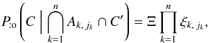 (12)where
 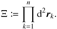 (13)
(13)
We now compute the second factor in the product of Eq. (6). Knowing the coordinates of K′-sources alone, without those of any in K, does not change the likelihood of the associations (Ak,jk); in other words, C′ and ![\hbox{$\bigcap_{\smash[t]{k=1}}^n A_{k\comma j_k}$}](/articles/aa/full_html/2014/06/aa20021-12/aa20021-12-eq102.png) are mutually unconditionally independent (but conditionally dependent on C). Therefore,
are mutually unconditionally independent (but conditionally dependent on C). Therefore,  (14)Let q := # { k ∈ [[1,n]] | jk ≠ 0 }, where #E denotes the number of elements of any set E. Since the events (Ak,jk)k ∈ [[1,n]] are independent by assumption (Hs:o),
  (15)Using definition (2), and on the hypothesis that all associations
  are a priori equally likely if k ≠ 0 (Sect. 2.2), we get
  (16)Since Ps:o(Ak, 0) = 1 − f, we have
  (17)Hence, from Eqs. (6), (12)and (17),
  (18)By the definition of q, there are q strictly positive indices jk (as many as the factors “
 ” in Eq. (18)) and n − q null ones (as many as the factors “(1 − f)”). Therefore, with
  (19)Eq. (18)reduces to
  (20)where the last equality is derived by induction from the distributivity of multiplication over addition.
3.1.2. Computation of Ps:o(Ai, j∩ C | C′)
The computation of the numerator of Eq. (4)is similar to that of Ps:o(C | C′):  (21)where we put ji := j.
Let q⋆ := # { k ∈ [[1,n]] | jk ≠ 0 } (indices jk are now those of Eq. (21)). As for Ps:o(C | C′),  (22)
(22)
3.1.3. Final results
Finally, from Eqs. (4), (20), and (22), fori ≠ 0, 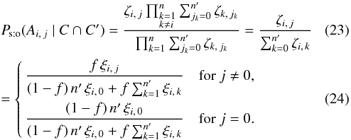
As to the probability Ps:o(A0,j | C ∩ C′) that has no counterpart in K, it can be computed in this way: 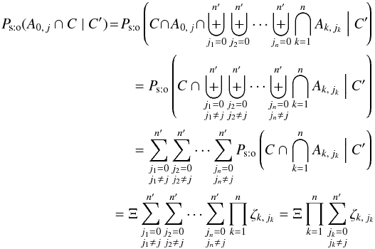 (25)and, using Eqs. (20), (23), and (3),
 ![\begin{eqnarray} \Psto(A_{0\comma j} \mid C \cap C') = \frac{ \Psto(A_{0\comma j} \cap C \mid C') }{ \Psto(C \mid C') } = \frac{\Xi\multspace \prod_{k=1}^n\sum_{\leftsubstack{j_k=0\\ j_k\neq j}}^\np \zeta_{k\comma j_k}}{\Xi\multspace \prod_{k=1}^n\sum_{j_k=0}^\np\zeta_{k\comma j_k}} \nonumber\\ = \prod_{k=1}^n\frac{\sum_{j_k=0}^\np\zeta_{k\comma j_k} - \zeta_{k\comma j}}{ \sum_{j_k=0}^\np\zeta_{k\comma j_k}} = \prod_{k=1}^n{\Biggl( 1-\frac{\zeta_{k\comma j_k}}{\sum_{j_k=0}^\np\zeta_{k\comma j_k}} \Biggr)} \nonumber\\= \prod_{k=1}^n{\left(1 - \Psto[A_{k\comma j} \mid C \cap C']\right)} \quad \text{for } j \neq 0. \label{P_sto(A0j|C,C)}\!\! \end{eqnarray}](/articles/aa/full_html/2014/06/aa20021-12/aa20021-12-eq133.png) (26)
(26)
3.2. Likelihood and estimation of unknown parameters
3.2.1. General results
Various methods have been proposed for estimating the fraction of sources with a counterpart (Kim et al. 2012; Fleuren et al. 2012; McAlpine et al. 2012; Haakonsen & Rutledge 2009). Pineau et al. (2011), for instance, fit f to the overall distribution of the likelihood ratios. We propose a more convenient and systematic method in this section.
Besides f, the probabilities P(Ai,j | C ∩ C′) may depend on other unknowns, such as the parameters  and
and  modeling the positional uncertainties (cf. Appendices A.2.2 and A.2.3). We write here x1, x2, etc., for all these parameters, and put x := (x1,x2,...). An estimate
  of x may be obtained by maximizing with respect to x (and with the constraint
 ![\hbox{$\hat f \in[0, 1]$}](/articles/aa/full_html/2014/06/aa20021-12/aa20021-12-eq141.png) ) the overall likelihood
) the overall likelihood ![\begin{equation} \label{def_Lh} \Lh \coloneqq \frac{\Prob(C \cap C')}{ (\prod_{i=1}^n \df^2\vec r_i)\multspace \prod_{j=1}^\np\df^2\vec r'_{\smash[t]{j}}} \end{equation}](/articles/aa/full_html/2014/06/aa20021-12/aa20021-12-eq142.png) (27)to observe all the K- and K′-sources at their effective positions. Unless the result is outside the possible domain for x (i.e., if L reaches its maximum on the boundary of this domain), the maximum likelihood estimator is a solution to
(27)to observe all the K- and K′-sources at their effective positions. Unless the result is outside the possible domain for x (i.e., if L reaches its maximum on the boundary of this domain), the maximum likelihood estimator is a solution to 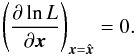 (28)From now on, all quantities calculated at
  bear a circumflex.
We have  (29)and, since clustering is neglected,
 ![\begin{equation} \label{P(C)} \Prob(C') = \prod_{j=1}^\np \Prob(\coordpj) = \prod_{j=1}^\np \xi_{0\comma j}\multspace \df^2\vec r'_{\smash[t]{j}}, \end{equation}](/articles/aa/full_html/2014/06/aa20021-12/aa20021-12-eq147.png) (30)where ξ0,j is the spatial probability density defined by
(30)where ξ0,j is the spatial probability density defined by ![\hbox{$\Prob(\coordpj) = \xi_{0\comma j}\multspace \df^2\vec r'_{\smash[t]{j}}$}](/articles/aa/full_html/2014/06/aa20021-12/aa20021-12-eq149.png) ; for the uninformative prior of a uniform a priori probability distribution of K′-sources, ξ0,j = 1 /S. From Eqs. (27), (29), (30), and (13), we obtain
; for the uninformative prior of a uniform a priori probability distribution of K′-sources, ξ0,j = 1 /S. From Eqs. (27), (29), (30), and (13), we obtain 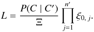 (31)
(31)
In particular, under assumption (Hs:o), Eqs. (31), (20), and (13)give 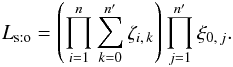 (32)Therefore, for any parameter xp and because the ξ0,j are independent of x,
 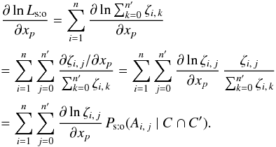 (33)(For reasons highlighted just after Eq. (73), it is convenient to express most results as a function of the probabilities P(Ai,j | C ∩ C′).)
Uncertainties on the unknown parameters may be computed from the covariance matrix V of . For large numbers of sources, V is asymptotically given (Kendall & Stuart 1979) by 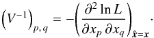 (34)
(34)
3.2.2. Fraction of sources with a counterpart
Consider, in particular, the case xp = f. We note that 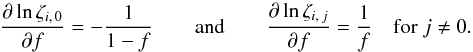 (35)Under the assumption (Hs:o) or (Ho:o) (but not under (Ho:s)),
  (36)so, using Eq. (35),
  (37)Summing Eq. (37)on i, we obtain from Eq. (33)that
  (38)Consequently, the maximum likelihood estimator of the fraction f of K-sources with a counterpart in K′ is
 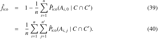 After some tedious calculations, it can be shown that
 ![\begin{equation} \label{concave} \frac{\partial^2\ln\Lhsto}{\partial f^2} = -\frac{ \sum_{i=1}^n{\left([1-f] - \Psto[A_{i\comma 0} \mid C \cap C']\right)^2} }{ f^2\multspace (1-f)^2 } < 0 \end{equation}](/articles/aa/full_html/2014/06/aa20021-12/aa20021-12-eq164.png) (41)for all f, so ∂lnLs:o/∂f has at most one zero in [0,1]:
(41)for all f, so ∂lnLs:o/∂f has at most one zero in [0,1]:  is unique.
Since appears on the two sides of Eq. (39)(remember that  is the value of Ps:o at
  ), we may try to determine it through an iterative back and forth computation between the lefthand and the righthand sides of this equation. (A similar idea was also proposed by Benn 1983.) We prove in Sect. 5.3 that this procedure converges for any starting value f ∈] 0,1 [.
An estimate  of the fraction f′ of K′-sources with a counterpart is given by
  (42)It can be checked from Eqs. (40), (42), and (26)that, as expected if assumption (Hs:o) is valid (cf. Sect. 2.2),
  . (Just notice that, for any numbers yi ∈ [0,1],
  , which is obvious by induction; apply this to
  and then sum on j.)
3.3. Probability of association: local computation
Under assumption (Hs:o), a purely local computation (subscript “loc” hereafter) of the probabilities of association is also possible. Consider a region Ui of area  containing the position of Mi, and such that we can safely hypothesize that the counterpart in K′ of Mi, if any, is inside. We assume that the local surface density
  of K′-sources unrelated to Mi is uniform on Ui. To avoid biasing the estimate if Mi has a counterpart, may be evaluated from the number of K′-sources in a region surrounding Ui, but not overlapping it (an annulus around a disk Ui centered on Mi, for instance).
Besides the Ai,j, we consider the following events:
-
 : Ui contains
  sources;
 -
 , where
  .
.
We want to compute the probability that a source in Ui is the counterpart of Mi, given the positions relative to Mi of all its possible counterparts ![\hbox{$(\Mp_k)^{}_{\smash[t]{k\in J_i}}$}](/articles/aa/full_html/2014/06/aa20021-12/aa20021-12-eq186.png) , i.e.
, i.e.  . Using Eq. (3)with ω1 = Ai,j,
  , and
, and  in the first equality below, and then with
  , ω2 = Ai,k, and ω3 unchanged in the last one, we obtain
 ![\begin{eqnarray} \Ploc(A_{i\comma j} \mid \COORDpi\cap \Npi) = \frac{\Ploc(A_{i\comma j} \cap \COORDpi \mid \Npi)}{ \Ploc(\COORDpi \mid \Npi)} \nonumber\\[1mm] = \frac{\Ploc(\COORDpi \cap A_{i\comma j} \mid \Npi)}{ \Ploc(\COORDpi \cap \biguplus_{k\in J_i\cup\{0\}} A_{i\comma k} \mid \Npi)} = \frac{\Ploc(\COORDpi \cap A_{i\comma j} \mid \Npi)}{ \sum_{k\in J_i\cup\{0\}} \Ploc(\COORDpi \cap A_{i\comma k} \mid \Npi)} \nonumber\\[1mm]= \frac{\Ploc(\COORDpi\mid A_{i\comma j} \cap \Npi)\multspace \Ploc(A_{i\comma j} \mid \Npi)}{ \sum_{k\in J_i\cup\{0\}} \Ploc(\COORDpi\mid A_{i\comma k} \cap \Npi) \multspace \Ploc(A_{i\comma k} \mid \Npi)}\cdot \label{P_loc(Aij|C,N)} \end{eqnarray}](/articles/aa/full_html/2014/06/aa20021-12/aa20021-12-eq192.png) (43)Now,
(43)Now,  (44)and
 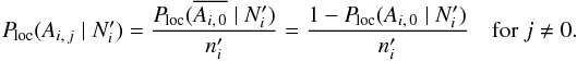 (45)(The probability Ploc(Ai,j) itself could not have been computed as
  because would be undefined, which is why event was introduced.) If clustering is negligible, the number of K′-sources randomly distributed with a mean surface density in an area follows a Poissonian distribution, so
 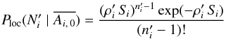 (46)(one counterpart and
  sources by chance in ) and
 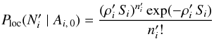 (47)(no counterpart and sources by chance in ). Thus, from Eqs. (45)–(47), and (2),
 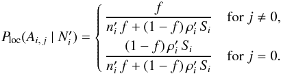 (48)We have
 ![\begin{eqnarray} \label{P_loc(C|Aij,N)} \Ploc(\COORDpi\mid A_{i\comma 0}\cap \Npi) = \prod_{k\in J_i} \frac{\df^2\vec r'_{\smash[t]{k}}}{\Si} \qquad\text{and}\qquad\nonumber\\ \Ploc(\COORDpi\mid A_{i\comma j} \cap \Npi) = \xi_{i\comma j}\multspace \df^2\vrpj\multspace \prod_{\substack{k\in J_i\\ k\neq j}} \frac{\df^2\vec r'_{\smash[t]{k}}}{\Si} \quad\text{for } j \neq 0 \end{eqnarray}](/articles/aa/full_html/2014/06/aa20021-12/aa20021-12-eq201.png) (49)(rigorously, ξi,j should be replaced by
(49)(rigorously, ξi,j should be replaced by 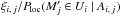 , but
, but  is negligible by definition of Ui), so, using Eqs. (43), (48), and (49), we obtain
 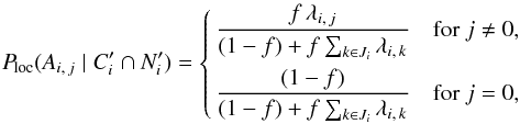 (50)where
  is the likelihood ratio (cf. Eq. (1)). Mutatis mutandis, we obtain the same result as Eq. (14) of Pineau et al. (2011) and the aforementioned authors. When the computation is extended from Ui to the whole surface covered by K′, is replaced by
  in Eq. (50), ∑ k ∈ Ji by
  , and we recover Eq. (24)since ξi, 0 = 1 /S for a uniform distribution.
The index jMLC(i) of the most likely counterpart  of Mi is the value of j ≠ 0 maximizing λi,j. Very often, λi,jMLC(i) ≫ ∑ k ∈ Ji; k ≠ jMLC(i)λi,k, so
 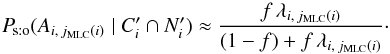 (51)As a “poor man’s” recipe, if the value of f is unknown and not too close to either 0 or 1, an association may be considered as true if λi,jMLC(i) ≫ 1 and as false if λi,jMLC(i) ≪ 1. Where to set the boundary between true associations and false ones is somewhat arbitrary (Wolstencroft et al. 1986). For a large sample, however, f can be estimated from the distribution of the positions of all sources, as shown in Sect. 3.2.
4. One-to-one associations
Under (Hs:o) (Sect. 3), a given can be associated with several Mi: there is no symmetry between K and K′ under this assumption and, while ![\hbox{$\sum_{\smash[t]{j=0}}^{\smash[t]{\np}} \Psto(A_{i\comma j}\mid C \cap C') = 1$}](/articles/aa/full_html/2014/06/aa20021-12/aa20021-12-eq220.png) for all Mi,
for all Mi, ![\hbox{$\sum_{\smash[t]{i=1}}^n \Psto(A_{i\comma j}\mid C \cap C')$}](/articles/aa/full_html/2014/06/aa20021-12/aa20021-12-eq221.png) could be strictly larger than 1 for some sources . We assume here that the much more constraining assumption (Ho:o) holds. As far as we know and despite some attempt by Rutledge et al. (2000), this problem has not been solved previously (see also Bartlett & Egret 1998 for a simple statement of the question).
could be strictly larger than 1 for some sources . We assume here that the much more constraining assumption (Ho:o) holds. As far as we know and despite some attempt by Rutledge et al. (2000), this problem has not been solved previously (see also Bartlett & Egret 1998 for a simple statement of the question).
Since a K′-potential counterpart of Mi within some neighborhood Ui of Mi might in fact be the true counterpart of another source Mkoutside of Ui, there is no obvious way to adapt the exact local several-to-one computation of Sect. 3.3 to the case of the one-to-one assumption. We therefore have to consider all the K- and K′-sources, as in Sect. 3.1.
Under assumption (Ho:o), catalogs K and K′ play symmetrical roles; in particular,  (52)For practical reasons (cf. Eq. (61)), we nonetheless name K the catalog with the fewer objects and K′ the other one, so
  in the following.
4.1. Probability of association
4.1.1. Computation of Po:o(C | C′)
The denominator of Eq. (4)is 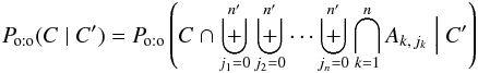 (53)(same reasons as for Eq. (6)). Because Ak,m ∩ Aℓ,m =? if k ≠ ℓ and m ≠ 0 by assumption (Ho:o), this reduces to
 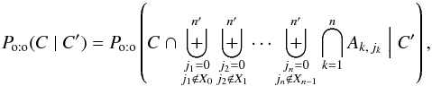 (54)where, to ensure that each K′-source is associated with at most one of K, the sets Xk of excluded counterparts are defined iteratively by
  (55)As a result,
 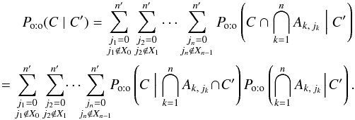 (56)The first factor in the product of Eq. (56)is still given by Eq. (12), so we just have to compute the second factor,
 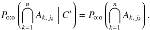 (57)Let
  and Q be a random variable describing the number of associations between K and K′:
  (58)Since
  by definition of q, we only have to compute
  and Po:o(Q = q).
There are n ! /(q ! [n − q] !) choices of q elements among n in K, and ![\hbox{$\np!/(q!\multspace [\np-q]!)$}](/articles/aa/full_html/2014/06/aa20021-12/aa20021-12-eq241.png) choices of q elements among in K′. The number of permutations of q elements is q !, so the total number of one-to-one associations of q elements from K to q elements of K′ is
choices of q elements among in K′. The number of permutations of q elements is q !, so the total number of one-to-one associations of q elements from K to q elements of K′ is  (59)The inverse of this number is
 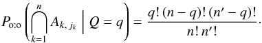 (60)With our definition of K and K′, , so all the elements of K may have a counterpart in K′ jointly. Therefore, Po:o(Q = q) is given by the binomial law:
 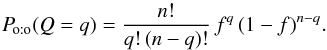 (61)From Eqs. (56), (12), (60), and (61), we obtain
 ![\begin{eqnarray} &&\Poto(C \mid C') \notag\\ &&= \Xi\multspace \sum_{\substack{j_1=0\\ j_1\not\in X_0}}^\np \sum_{\substack{j_2=0\\ j_2\not\in X_1}}^\np \cdots \sum_{\substack{j_n=0\\ j_n\not\in X_{n-1}}}^\np {\frac{(\np-q)!}{\np!} \multspace f^q \multspace (1-f)^{n-q}\multspace \prod_{k=1}^n \xi_{k\comma j_k}} ~~~~~~~~~~~~~~~~~ \\ &&= \Xi\multspace \sum_{\substack{j_1=0\\ j_1\not\in X_0}}^\np \sum_{\substack{j_2=0\\ j_2\not\in X_1}}^\np \cdots \sum_{\substack{j_n=0\\ j_n\not\in X_{n-1}}}^\np {\Left(\prod_{\ell=1}^q\frac{f}{\np-\ell+1}\Right)\multspace \Left(\prod_{\ell=1}^{n-q}[1-f]\Right)\multspace \prod_{k=1}^n \xi_{k\comma j_k}}.~~~~~~~~~~~~~~~~~ \label{P_oto(C|C)_eta} \end{eqnarray}](/articles/aa/full_html/2014/06/aa20021-12/aa20021-12-eq246.png) There are q factors “
There are q factors “ ” in the above equation, one for each index jk ≠ 0. There are also n − q factors “(1 − f)”, one for each null jk. For every jk ≠ 0,
  ; and, since
  , a different jk corresponds to each ℓ ∈ [[1,q]], so
  . With
 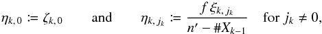 (64)Eq. (63)therefore simplifies to
 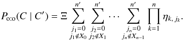 (65)
(65)
4.1.2. Computation of Po:o(Ai, j∩ C | C′)
The denominator of Eq. (4)is computed in the same way as Po:o(C | C′): 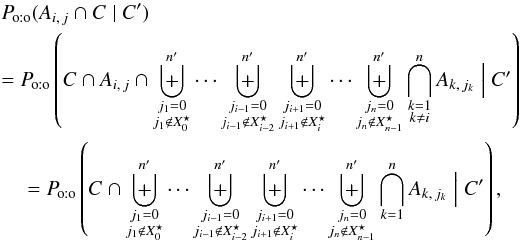 (66)where
 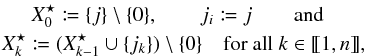 (67)so
 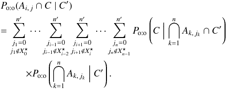 (68)Let
  . As for Po:o(C | C′),
 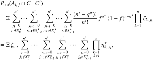 (69)where
 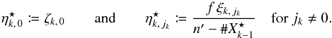 (70)
(70)
4.1.3. Final results
Finally, from Eqs. (4), (65), and (69), fori ≠ 0, 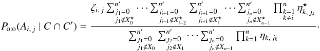 (71)
(71)
The probability that a source has no counterpart in K is simply given by 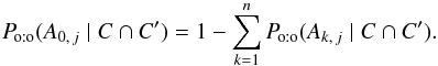 (72)
(72)
4.2. Likelihood and estimation of unknown parameters
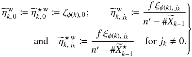
As in Sect. 3.2, an estimate  of the set x of unknown parameters may be obtained by solving Eq. (28). Under assumption (Ho:o), we obtain from Eqs. (65), (31), and (13)that
 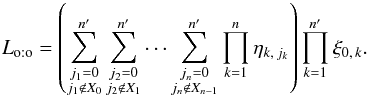 (73)Because the number of terms in Eq. (73)grows exponentially with n and , this equation seems useless. In fact, the prior computation of Lo:o is not necessary if the probabilities Po:o(Ai,j | C ∩ C′) are calculable (we see how to evaluate these in Sect. 5.4).
Indeed, for any parameter xp, we get the same result (Eq. (33)) as under assumption (Hs:o). First, we note that, since the ξ0,j are independent of x, we obtain from Eq. (31)that 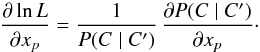 (74)Now, for any set Υ of indices and any product of strictly positive functions hk of some variable y,
 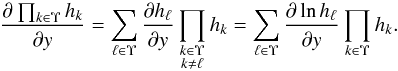 (75)With hk = ηk,jk, y = xp and Υ = [[1,n]], we therefore obtain from Eq. (65)that
 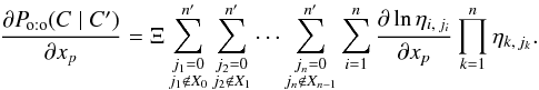 (76)The expression of Po:o(Ai,j ∩ C | C′) (Eq. (69)) may also be written
 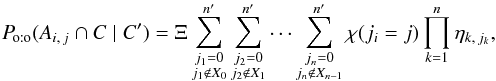 (77)where χ is the indicator function (i.e. χ(ji = j) = 1 if proposition “ji = j” is true and χ(ji = j) = 0 otherwise), so
 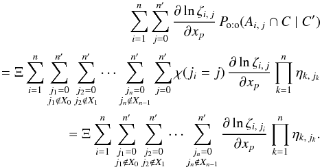 (78)If ji = 0, then ηi,ji = ζi,ji; and if ji ≠ 0, the numerators of ηi,ji and ζi,ji are the same and their denominators do not depend on xp: in all cases, ∂lnηi,ji/∂xp = ∂lnζi,ji/∂xp. The righthand sides of Eqs. (76)and (78)are therefore identical. Dividing their lefthand sides by Po:o(C | C′) and using Eqs. (74)and (4), we obtain, as announced,
 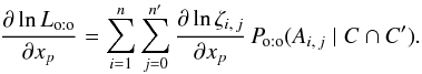 (79)
(79)
For xp = f in particular, because of Eq. (37), and as under assumption (Hs:o), Eq. (79)reduces to  (80)From Eq. (28), a maximum likelihood estimator of f is thus
 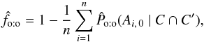 (81)where
  is the value of Po:o at
  .
.
To compare assumptions (Hs:o), (Ho:o), and (Hs:o) and to select the most appropriate one to compute P(Ai,j | C ∩ C′), an expression is needed for Lo:o. If probabilities Po:o(Ai, 0 | C ∩ C′) are calculable, Lo:o may be obtained for any f by integrating Eq. (80)with respect to f. Since all K- and K′-sources are unrelated and randomly distributed for f = 0, the integration constant is (cf. Eq. (73)) 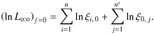 (82)
(82)
5. Practical implementation: the Aspects code
5.1. Overview
To implement the results established in Sects. 3.1, 3.2, 4.1, and 4.2, we have built a Fortran 95 code, Aspects – a French acronym (pronounced [aspε] in International Phonetic Alphabet, not [æspekts]) for “Association positionnelle/probabiliste de catalogues de sources”, or “probabilistic positional association of source catalogs” in English. The source files are freely available 4 at www2.iap.fr/users/fioc/Aspects/ . The code compiles with IFort and GFortran.
Given two catalogs of sources with their positions and the uncertainties on these, Aspects computes, under assumptions (Hs:o), (Ho:o), and (Ho:s), the overall likelihood L, estimates of f and f′, and the probabilities P(Ai,j | C ∩ C′). It may also simulate all-sky catalogs for various association models (cf. Sect. 6.1).
We provide hereafter explanations of general interest for the practical implementation in Aspects of Eqs. (23), (39), (32), (71), (81), and (73). Some more technical points (such as the procedures used to search for nearby objects, simulate the positions of associated sources and integrate Eq. (80)) are only addressed in appendices to the documentation of the code (Fioc 2014). The latter also contains the following complements: another (but equivalent) expression for Lo:o, formulae derived under Ho:s, computations under Ho:o for  , a calculation of the uncertainties on unknown parameters under Hs:o, and a proof of Eq. (41).
5.2. Elimination of unlikely counterparts
Under assumption (Hs:o), computing the probability of association Ps:o(Ai,j | C ∩ C′) between Mi and from Eq. (23)is straightforward if f and the positional uncertainties are known. However, the number of calculations for the whole sample or for determining is on the order of  , a huge number for the catalogs available nowadays. We must therefore try to eliminate all unnecessary computations.
Since ξi,k is given by a normal law if i ≠ 0 and k ≠ 0, it rapidly drops to almost 0 when we consider sources  at increasing angular distance ψi,k from Mi. Therefore, there is no need to compute Ps:o(Ai,j | C ∩ C′) for all couples
  or to sum on all k from 1 to in Eq. (24). More explicitly, let R′ be some angular distance such that, for all
  , if
, if  then ξi,k ≈ 0, say
 ![\begin{equation} \label{def_R} R' \ga 5\multspace \!\sqrt{ \smash[b]{ \max_{\ell\in\integinterv{1}{n}} a_\ell^2 + \max_{\ell\in\integinterv{1}{\np}} a_{\ell}'^2 } }, \vphantom{ \max_{\ell\in\integinterv{1}{n}} a_\ell^2 + \max_{\ell\in\integinterv{1}{\np}} a_{\ell}'^2 } \end{equation}](/articles/aa/full_html/2014/06/aa20021-12/aa20021-12-eq313.png) (83)where the aℓ and
(83)where the aℓ and ![\hbox{$a'_{\smash[t]{\ell}}$}](/articles/aa/full_html/2014/06/aa20021-12/aa20021-12-eq315.png) are the semi-major axes of the positional uncertainty ellipses of K- and K′-sources (cf. Appendix A.2.1; the square root in Eq. (83)is thus the maximal possible uncertainty on the relative position of associated sources). We may set Ps:o(Ai,j | C ∩ C′) to 0 if ψi,j>R′, and replace the sums
are the semi-major axes of the positional uncertainty ellipses of K- and K′-sources (cf. Appendix A.2.1; the square root in Eq. (83)is thus the maximal possible uncertainty on the relative position of associated sources). We may set Ps:o(Ai,j | C ∩ C′) to 0 if ψi,j>R′, and replace the sums ![\hbox{$\smash[t]{\sum_{\smash[t]{k=1}}^\np}$}](/articles/aa/full_html/2014/06/aa20021-12/aa20021-12-eq317.png) by
by ![\hbox{$\smash[t]{\sum_{\smash[t]{k=1{;}\, \psi_{i\comma k}\leqslant R'}}^\np}$}](/articles/aa/full_html/2014/06/aa20021-12/aa20021-12-eq318.png) in Eq. (24): only nearby K′-sources matter.
in Eq. (24): only nearby K′-sources matter.
5.3. Fraction of sources with a counterpart
All the probabilities depend on f and, possibly, on other unknown parameters like and (cf. Appendices A.2.2 and A.2.3). Under assumption (Hs:o), estimates of these parameters may be found by solving Eq. (28)using Eq. (33).
If the fraction of sources with a counterpart is the only unknown, the ξi,j need to be computed only once and may easily be determined from Eq. (39)by an iterative procedure. Denoting by g the function ![\begin{equation} \label{fonction_g} g\colon f \in [0, 1] \longmapsto 1-\frac{1}{n}\multspace \sum_{i=1}^n\Psto(A_{i\comma 0} \mid C \cap C'), \end{equation}](/articles/aa/full_html/2014/06/aa20021-12/aa20021-12-eq320.png) (84)we now prove that, for any f0 ∈] 0,1 [, the sequence (fk)k ∈? defined by fk + 1 := g(fk) tends to .
(84)we now prove that, for any f0 ∈] 0,1 [, the sequence (fk)k ∈? defined by fk + 1 := g(fk) tends to .
As is obvious from Eq. (24b), Ps:o(Ai, 0 | C ∩ C′) decreases for all i when f increases: g is consequently an increasing function. Note also that, from Eqs. (38)and (84),  (85)The only fixed points of g are thus 0, 1 and the unique solution to ∂lnLs:o/∂f = 0. Because ∂2lnLs:o/∂f2< 0 (cf. Eq. (41)) and
  , we have
  if
if ![\hbox{$f \in [0, \hat f_\sto]$}](/articles/aa/full_html/2014/06/aa20021-12/aa20021-12-eq330.png) , so
, so  in this interval by Eq. (85). Similarly, if
 ![\hbox{$f \in [\hat f_\sto, 1]$}](/articles/aa/full_html/2014/06/aa20021-12/aa20021-12-eq332.png) , then
, then  and thus
  .
.
Consider the case ![\hbox{$f_0 \in \mathopen{]}0, \hat f_\sto]$}](/articles/aa/full_html/2014/06/aa20021-12/aa20021-12-eq335.png) . If
. If  , then as just shown,
  ; we also have
  , because g is an increasing function and is a fixed point of it. Since g(fk) = fk + 1, the sequence (fk)k ∈? is increasing and bounded from above by : it therefore converges in
 ![\hbox{$[f_0, \hat f_\sto]$}](/articles/aa/full_html/2014/06/aa20021-12/aa20021-12-eq340.png) . Because g is continuous and is the only fixed point in this interval, (fk)k ∈? tends to . Similarly, if
. Because g is continuous and is the only fixed point in this interval, (fk)k ∈? tends to . Similarly, if  , then (fk)k ∈? is a decreasing sequence converging to .
Because of Eq. (81), this procedure also works in practice under assumption (Ho:o) (with Ps:o replaced by Po:o in Eq. (84)), although it is not obvious that Po:o(Ai, 0 | C ∩ C′) decreases for all i when f increases, nor that ∂2lnLo:o/∂f2< 0. A good starting value f0 may be .
5.4. Computation of one-to-one probabilities of association
What was said in Sect. 5.2 about eliminating unlikely counterparts in the calculation of probabilities under Hs:o still holds under Ho:o. However, because of the combinatorial explosion of the number of terms in Eq. (71), computing Po:o(Ai,j | C ∩ C′) exactly is still clearly hopeless. Yet, after some wandering (Sects. 5.4.1 and 5.4.2), we found a working solution (Sect. 5.4.3).
5.4.1. A first try
Our first try was inspired by the (partially wrong) idea that, although all K-sources are involved in the numerator and denominator of Eq. (71), only those close to Mi should matter in their ratio. A sequence of approximations converging to the true value of Po:o(Ai,j | C ∩ C′) might then be built as follows (all quantities defined or produced in this first try are written with the superscript “w” for “wrong”).
To make things clear, consider M1 and some possible counterpart within its neighborhood ( ) and assume that M2 is the first nearest neighbor of M1 in K, M3 its second nearest neighbor, etc. For any d ∈ [[1,n]], define
 ![\begin{equation} p^\wrong_{\smash[t]{d}}(1, j) \coloneqq \frac{ \zeta_{1\comma j}\multspace \sum_{\leftsubstack{j_2=0\\ j_2\not\in X^{\star}_1}}^\np \cdots \sum_{\leftsubstack{j_d=0\\ j_d\not\in X^{\star}_{d-1}}}^\np \prod_{k=2}^d \eta^{\star}_{k\comma j_k} }{ \sum_{\leftsubstack{j_1=0\\ j_1\not\in X_0}}^\np \sum_{\leftsubstack{j_2=0\\ j_2\not\in X_1}}^\np \cdots \sum_{\leftsubstack{j_d=0\\ j_d\not\in X_{d-1}}}^\np \prod_{k=1}^d \eta_{k\comma j_k} }\cdot \end{equation}](/articles/aa/full_html/2014/06/aa20021-12/aa20021-12-eq349.png) (86)The quantity
(86)The quantity ![\hbox{$p^\wrong_{\smash[t]{d}}(1, j)$}](/articles/aa/full_html/2014/06/aa20021-12/aa20021-12-eq350.png) thus depends only on M1 and its d − 1 nearest neighbors in K. As
thus depends only on M1 and its d − 1 nearest neighbors in K. As  is the one-to-one probability of association between M1 and (cf. Eq. (71)), the sequence
 ![\hbox{$(p^\wrong_{\smash[t]{d}}[1, j])$}](/articles/aa/full_html/2014/06/aa20021-12/aa20021-12-eq353.png) tends to Po:o(A1,j | C ∩ C′) when the depth d of the recursive sums tends to n. After some initial fluctuations, enters a steady state. This occurs when ψ(M1,Md + 1) exceeds a distance R equal to a few times R′ (at least 2 R′). We may therefore think that the convergence is then achieved and stop the recursion at this d. It is all the more tempting that
tends to Po:o(A1,j | C ∩ C′) when the depth d of the recursive sums tends to n. After some initial fluctuations, enters a steady state. This occurs when ψ(M1,Md + 1) exceeds a distance R equal to a few times R′ (at least 2 R′). We may therefore think that the convergence is then achieved and stop the recursion at this d. It is all the more tempting that  and that the several-to-one probability looks like a first-order approximation to Po:o...
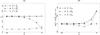 |
Fig. 1 One-to-one simulations for f = 1/2, |


More formally and generally, for any Mi, let φ be a permutation on K ordering the elements Mφ(1), Mφ(2), ..., Mφ(n) by increasing angular distance to Mi (in particular, Mφ(1) = Mi). For j = 0 or within a distance R′ (cf. Sect. 5.2) from Mi, and for any d ∈ [[1,n]], define ![\begin{equation} \label{P_oto_iter_w} p^\wrong_{\smash[t]{d}}(i, j) \coloneqq \frac{ \zeta_{i\comma j}\multspace\sum_{\leftsubstack{j_2=0\\ j_2\not\in \widetilde X^{\star}_1}}^\np \cdots \sum_{\leftsubstack{j_d=0\\ j_d\not\in \widetilde X^{\star}_{d-1}}}^\np \prod_{k=2}^d \widetilde\eta^{\,\star\,\wrong}_{k\comma j_k} }{ \sum_{\leftsubstack{j_1=0\\ j_1\not\in \widetilde X_0}}^\np \sum_{\leftsubstack{j_2=0\\ j_2\not\in \widetilde X_1}}^\np \cdots \sum_{\leftsubstack{j_d=0\\ j_d\not\in \widetilde X_{d-1}}}^\np \prod_{k=1}^d \widetilde\eta^{\,\wrong}_{k\comma j_k} }, \vspace*{3mm} \end{equation}](/articles/aa/full_html/2014/06/aa20021-12/aa20021-12-eq372.png) (87)where, as in Eqs. (55), (67), (64), and (70),
(87)where, as in Eqs. (55), (67), (64), and (70),
 (88)
(88) (89)Let
 ![\begin{equation} \label{min_prof} \depthmin(i) \coloneqq \min\left(d \in \integinterv{1}{n} \bigm| \psi[M_i, M_{\phi(d+1)}] > R\right). \end{equation}](/articles/aa/full_html/2014/06/aa20021-12/aa20021-12-eq375.png) (90)Given above considerations, Po:o(Ai,j | C ∩ C′) can be evaluated as
(90)Given above considerations, Po:o(Ai,j | C ∩ C′) can be evaluated as ![\hbox{$p^\wrong_\oto(i, j) \coloneqq p^\wrong_{\smash[t]{\depthmin(i)}}(i, j)$}](/articles/aa/full_html/2014/06/aa20021-12/aa20021-12-eq376.png) .
.
The computation of ![\hbox{$p^\wrong_{\smash[t]{d}}(i, j)$}](/articles/aa/full_html/2014/06/aa20021-12/aa20021-12-eq377.png) may be further restricted (and in practice, because of the recursive sums in Eq. (87), must be) to sources
may be further restricted (and in practice, because of the recursive sums in Eq. (87), must be) to sources  in the neighborhood of the objects (Mφ(k))k ∈ [[1,d]], as explained in Sect. 5.2.
5.4.2. Failure of the first try
To test the reliability of the evaluation of Po:o(Ai,j | C ∩ C′) by  , we simulated all-sky mock catalogs for one-to-one associations and analyzed them with a first version of Aspects. Simulations were run for f = 1/2,
  ,
,  , and known circular positional uncertainties with
  (see Sects. 6.1 and 6.2 for a detailed description).
Three estimators of f were compared to the input value:
-
, the value maximizing Ls:o (Eq. (39));
-
 , the value maximizing the one-to-one likelihood
  derived from the
  . This estimator is computed from Eq. (81)with
  instead of Po:o(Ai, 0 | C ∩ C′);
 -
 , an estimator built from the one-to-several assumption in the following way: because (Ho:s) is fully symmetric to (Hs:o), we just need to swap K and K′ (i.e., swap f and f′, n and , etc.) in Eqs. (24), (26), and (39)to obtain
  instead of , and then, from Eq. (42), instead of . The one-to-several likelihood Lo:s is computed from Eq. (32)in the same way.
The mean values of these estimators are plotted as a function of n in Fig. 1a (error bars are smaller than the size of the points). As is obvious, the ad hoc estimator diverges from f when n increases. This statistical inconsistency 5 seems surprising for a maximum likelihood estimator since the model on which it is based is correct by construction. However, all the demonstrations of consistency of maximum likelihood estimators we found in the literature (e.g., in Kendall & Stuart 1979) rest on the assumption that the overall likelihood is the product of the probabilities of each datum, which is not the case for Lo:o (cf. Eq. (73)). Since is a good estimator of f, it might be used to compute Po:o(Ai,j | C ∩ C′) from – if the latter correctly approximates the former. By itself, the inconsistency of  is therefore not a problem.
More embarrassing is that (Ho:o) is not the most likely assumption (see Fig. 1b): the mean value of  is less than that of
  over the full interval of n ! These two failures hint that the sequence
 ![\hbox{$(p^\wrong_{\smash[t]{d}}[i, j])$}](/articles/aa/full_html/2014/06/aa20021-12/aa20021-12-eq393.png) has not yet converged to Po:o(Ai,j | C ∩ C′) at d = dmin(i).
has not yet converged to Po:o(Ai,j | C ∩ C′) at d = dmin(i).
To check this, we ran simulations with small numbers of sources (n and less than 10), so that we could compute  exactly and study how
 ![\hbox{$(p^\wrong_{\smash[b]d}[i, j])$}](/articles/aa/full_html/2014/06/aa20021-12/aa20021-12-eq397.png) tends to it. To test whether source confusion might be the reason for the problem, we created mock catalogs with very large positional uncertainties 6, comparable to the distance between unrelated sources. Because the expressions given in Appendix A for ξi,j are for planar normal laws and become wrong when the distance between Mi and is more than a few degrees because of the curvature, we ran simulations on a whole circle instead of a sphere; nevertheless, we took
tends to it. To test whether source confusion might be the reason for the problem, we created mock catalogs with very large positional uncertainties 6, comparable to the distance between unrelated sources. Because the expressions given in Appendix A for ξi,j are for planar normal laws and become wrong when the distance between Mi and is more than a few degrees because of the curvature, we ran simulations on a whole circle instead of a sphere; nevertheless, we took  because the linear normal law is inappropriate on a circle for higher values, due to its finite extent. What we found is that, after the transient phase where it oscillates, slowly drifts to Po:o(Ai,j | C ∩ C′) and only converges at d = n ! This drift was imperceptible for the high values of n and used in Sect. 5.4.1.
5.4.3. Reconsideration and solution
To understand where the problem comes from, we consider the simplest case of interest:  . We assume moreover that ξ1, 2 ≈ ξ2, 1 ≈ 0. We then have
 ![\begin{eqnarray} \Poto(C \mid C') \approx \Biggl([1-f]^2\multspace \xi_{1\comma 0}\multspace \xi_{2\comma 0} + \frac{[1-f]\multspace f}{2}\multspace [\xi_{1\comma 0}\multspace \xi_{2\comma 2} + \xi_{1\comma 1}\multspace \xi_{2\comma 0}] \nonumber \\ +\frac{f^2}{2}\multspace \xi_{1\comma 1}\multspace \xi_{2\comma 2}\Biggr) \multspace \df^2\vec r_1\multspace \df^2\vec r_2, \end{eqnarray}](/articles/aa/full_html/2014/06/aa20021-12/aa20021-12-eq402.png) (91)
(91)![\begin{eqnarray} && \Poto(A_{1\comma 0} \cap C \mid C') \approx (1\!-\!f)\multspace \xi_{1\comma 0}\multspace \Biggl([1\!-\!f]\multspace \xi_{2\comma 0} + \frac{f}{2}\multspace \xi_{2\comma 2}\Biggr) \multspace \df^2\vec r_1\multspace \df^2\vec r_2, ~~~~~~~~~~~~~~~~~~~~~~~\\ &&\Poto(A_{1\comma 1} \cap C \mid C') \approx \frac{f}{2}\multspace \xi_{1\comma 1}\multspace \left([1-f]\multspace \xi_{2\comma 0} + f\multspace \xi_{2\comma 2}\right)\multspace \df^2\vec r_1 \multspace \df^2\vec r_2.~~~~~~~~~~~~~~~~~~~~~~~ \end{eqnarray}](/articles/aa/full_html/2014/06/aa20021-12/aa20021-12-eq403.png) The probabilities Po:o(A1,j | C ∩ C′) = Po:o(A1,j ∩ C | C′) /Po:o(C | C′) obviously depend on ξ2, 2. In particular, ifξ2, 2 ≪ ξ2, 0,
The probabilities Po:o(A1,j | C ∩ C′) = Po:o(A1,j ∩ C | C′) /Po:o(C | C′) obviously depend on ξ2, 2. In particular, ifξ2, 2 ≪ ξ2, 0, 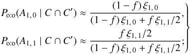 (94)in that case, Po:o(A2, 2 | C ∩ C′) ≈ 0, and both
  and
and  are free for M1. On the other hand, ifξ2, 2 ≫ ξ2, 0,
 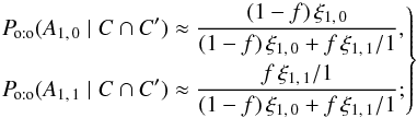 (95)in that case, Po:o(A2, 2 | C ∩ C′) ≈ 1: M2 and
  are almost certainly bound, so may not be associated to M1, and
  is the only possible counterpart of M1.
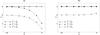 |
Fig. 2 Mean value of different estimators |
The difference between the results obtained for ξ2, 2 ≪ ξ2, 0 and ξ2, 2 ≫ ξ2, 0 shows that probabilities Po:o(A1,j | C ∩ C′) depend on the relative positions of M2 and , even when both M2 and are distant from M1 and : unlike the idea stated in Sect. 5.4.1, distant K-sources do matter for Po:o probabilities! However, as highlighted by the “/ 2” and “/ 1” factors in Eqs. (94)and (95), the distant K-source M2 only changes the number of K′-sources (two for ξ2, 2 ≪ ξ2, 0, one for ξ2, 2 ≫ ξ2, 0) that may be identified to M1: its exact position is unimportant.
This suggests the following solution: replace in Eq. (89)by the number  of K′-sources that may effectively be associated to Mi and its d − 1 nearest neighbors in K; i.e., dropping the superscript “w”, define
 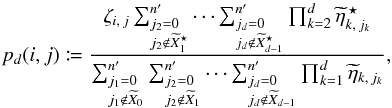 (96)where
 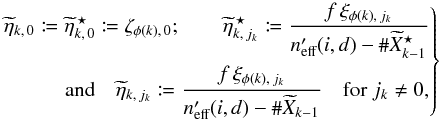 (97)and use po:o(i,j) := pdmin(i)(i,j), where dmin(i) is defined by Eq. (90), to evaluate Po:o(Ai,j | C ∩ C′).
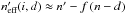
An estimate of  is given by 7
![\begin{equation} \label{n_eff} \npeff(i,d) = \np - \sum_{k=d+1}^n{\left(1 - \Poto[A_{\phi(k)\comma0} \mid C \cap C']\right)}. \end{equation}](/articles/aa/full_html/2014/06/aa20021-12/aa20021-12-eq425.png) (98)The sum in Eq. (98)is nothing but the typical number of counterparts in K′ associated to distant K-sources. Note that
(98)The sum in Eq. (98)is nothing but the typical number of counterparts in K′ associated to distant K-sources. Note that  , so we recover the theoretical result for Po:o(Ai,j | C ∩ C′) when all sources are considered. As Po:o depends on which in turn depends on Po:o, both may be computed with a back and forth iteration; this procedure converges in a few steps if, instead of Po:o, the value of Ps:o is taken to initiate the sequence.
5.5. Tests of Aspects
As computations made under assumption (Ho:o) are complex (they involve recursive sums for instance), we made several consistency checks of the code. In particular, we swapped K and K′ for  and compared quantities resulting from this swap (written with the superscript “↔”) to original ones: within numerical errors,
  and, for f′ ↔ = f, we get
  and
and  for all .
We moreover numerically checked for small n and (≲5) that Eq. (73)and the integral of Eq. (80)with respect to f are consistent and that Aspects returns the same value as Mathematica (Wolfram 1996). For even smaller n and ( 3), we confirmed that manual analytical expressions, obtained from the enumeration of all possible associations between K and K′, are identical to Mathematica’s symbolic calculations. For the large n and of practical interest, although we did not give a formal proof of the solution of Sect. 5.4.3, the analysis of simulations (Sect. 6) makes us confident in the code.
6. Simulations
In this section, we analyze various estimators of the unknown parameters. Because of the complexity of the expressions we obtained, we did not try to do it analytically but used simulations. We also compare the likelihood of the assumptions (Hs:o), (Ho:o), and (Ho:s), given the data.
6.1. Creation of mock catalogs
We have built all-sky mock catalogs with Aspects in the cases of several- and one-to-one associations. To do this, we first selected the indices of fn objects in K, and associated randomly the index of a counterpart in K′ to each of them; for one-to-one simulations, a given K′-source was associated at most once. We then drew the true positions of K′-sources uniformly on the sky. The true positions of K-sources without counterpart were also drawn in the same way; for sources with a counterpart, we took the true position of their counterpart. The observed positions of K- and K′-sources were finally computed from the true positions for given parameters (ai,bi,βi) and ![\hbox{$(a'_{\smash[t]{j}}, b'_{\smash[t]{j}}, \betapj)$}](/articles/aa/full_html/2014/06/aa20021-12/aa20021-12-eq437.png) of the positional uncertainty ellipses (see Appendix A.2.1).
of the positional uncertainty ellipses (see Appendix A.2.1).
6.2. Estimation of f if positional uncertainty ellipses are known and circular
Mock catalogs were created with ai = bi = σ (see notations in Appendix A.2.1) for all Mi ∈ K and with ![\hbox{$a'_{\smash[t]{j}} = b'_{\smash[t]{j}} = \sigma'$}](/articles/aa/full_html/2014/06/aa20021-12/aa20021-12-eq440.png) for all
for all  . Positional uncertainty ellipses are therefore circular here. Only two parameters matter in that case: f and
 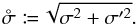 (99)Hundreds of simulations were run for f = 1/2,
  , , and n ∈ [[103, 105]]. We analyzed them with Aspects, knowing positional uncertainties, and plot the mean value of the estimators of f listed in Sect. 5.4.2 as a function of n in Fig. 2. This time, however, we replaced by the estimator
  computed from the po:o.
For several-to-one simulations, is by far the best estimator of f and does not show any significant bias, whatever the value of n. Estimators and do not recover the input value of f, which is not surprising since they are not built from the right assumption here; moreover, while , , and are obtained by maximizing Ls:o, Lo:s, and Lo:o, respectively, is not directly fitted to the data.
For one-to-one simulations, and unlike , is a consistent estimator of f, as expected. Puzzlingly, also works very well, maybe because (Hs:o) is a more relaxed assumption than (Ho:o); whatever the reason, this is not a problem.
6.3. Simultaneous estimation of f and
6.3.1. Circular positional uncertainty ellipses
How do different estimators of f and behave when the true values of positional uncertainties are also ignored? We show in Fig. 3 the result of simulations with the same input as in Sect. 6.2, except that  . The likelihood Ls:o peaks very close to the input value of
  for both types of simulations:
  is still an unbiased estimator of x. For one-to-one simulations, Lo:o is also maximal near the input value of x, so is unbiased, too.
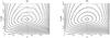 |
Fig. 3 Contour lines of Ls:o (solid) and Lo:o (dashed) in the |

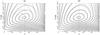 |
Fig. 4 Contour lines of Ls:o (solid) and Lo:o (dashed) in the |
6.3.2. Elongated positional uncertainty ellipses
To test the robustness of estimators of f, we ran simulations with the same parameters, but with elongated positional uncertainty ellipses: we took ![\hbox{$a_i = a'_{\smash[t]{j}} = 1.5\times10^{-3}\,\radian$}](/articles/aa/full_html/2014/06/aa20021-12/aa20021-12-eq449.png) and
and ![\hbox{$b_i = b'_{\smash[t]{j}} = a_i/3$}](/articles/aa/full_html/2014/06/aa20021-12/aa20021-12-eq450.png) for all . These ellipses were randomly oriented; i.e., position angles (cf. Appendix A.2.1) βi and
for all . These ellipses were randomly oriented; i.e., position angles (cf. Appendix A.2.1) βi and  have uniform random values in [0,ß [. We then estimated f, but ignoring these positional uncertainties (see Fig. 4).
Although the model from which the parameters are fitted is inaccurate here (the ξi,j are computed assuming circular positional uncertainties instead of the unknown elliptical ones), the input value of f is still recovered by for both types of simulations and by for one-to-one simulations. The fitting also provides the typical positional uncertainty on the relative positions of associated sources.
6.4. Choice of association model
Now, given the two catalogs, which assumption should we adopt to compute the probabilities P(Ai,j | C ∩ C′): several-to-one, one-to-one or one-to-several? As shown in Fig. 5, for known positional uncertainties and a given , source confusion is rare at low values of n (there is typically at most one possible counterpart) and all assumptions are equally likely. At larger n,  for several-to-one simulations; as expected, for one-to-one simulations,
  and
and  , with
  for
for  . In all cases, on average, the right assumption is the most likely. This is also true when positional uncertainties are ignored (Sect. 6.3).
The calculation of Lo:o is lengthy, and as a substitute to the comparison of the likelihoods, the following procedure may be applied to select the most appropriate assumption to compute the probabilities of association: if  , use (Ho:o); if
  , then use (Hs:o) if
  , and (Ho:s) otherwise.
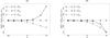 |
Fig. 5 Normalized average maximum value |

7. Conclusion
In this paper, we computed the probabilities of positional association of sources between two catalogs K and K′ under two different assumptions: first, the easy case where several K-objects may share the same counterpart in K′, then the more natural but numerically intensive case of one-to-one associations only between K and K′.
These probabilities depend on at least one unknown parameter: the fraction of sources with a counterpart. If the positional uncertainties are unknown, other parameters are required to compute the probabilities. We calculated the likelihood of observing all the K- and K′-sources at their effective positions under each of the two assumptions described above, and estimated the unknown parameters by maximizing these likelihoods. The latter are also used to select the best association model.
These relations were implemented in a code, Aspects, which we make public and with which we analyzed all-sky several-to-one and one-to-one simulations. In all cases, the assumption with the highest likelihood is the right one, and estimators of unknown parameters obtained for it do not show any bias.
In the simulations, we assumed that the density of K- and K′-sources was uniform on the sky area S: the quantities ξi, 0 and ξ0,j used to compute the probabilities are then equal to 1 /S. If the density of objects is not uniform, we might take ξi, 0 = ρ(Mi) /n and  , where ρ and ρ′ are, respectively, the local surface densities of K- and K′-sources; but if the ρ′rho ratio varies on the sky, so will the fraction of sources with a counterpart – something we did not try to model. Considering clustering or the side effects 8 due to a small S, as well as taking priors on the SED of objects into account was also beyond the scope of this paper.
In spite of these limitations, Aspects is a robust tool that should help astronomers cross-identify astrophysical sources automatically, efficiently and reliably.
For instance, de Ruiter et al. (1977) wrongly state that, if there is a counterpart, the closest object is always the right one.
For the sake of clarity, we mention that we adopt the same decreasing order of precedence for operators as in Mathematica (Wolfram 1996): × and /; Π; ∑; + and −.
Computing Ps:o(C | C′) is easier than for Ps:o(C′ | C): the latter would require calculating ![\hbox{$\Psto(c'_{\smash[t]{\ell}} \mid \bigcap_{\smash[t]{k=1{;}\, j_k=\ell}}^n {[c_k \cap A_{k\comma j_k}]})$}](/articles/aa/full_html/2014/06/aa20021-12/aa20021-12-eq592.png) (cf. Eq. (9)) because several Mk might be associated with the same
(cf. Eq. (9)) because several Mk might be associated with the same  . This does not matter for computations made under assumption (Ho:o).
Fortran 90 routines from Numerical Recipes (Press et al. 1992) are used to sort arrays and locate a value in an ordered table. Because of license constraints, we cannot provide them, but they may easily be replaced by free equivalents.

None of the results established outside of Appendix A depends on this assumption.
If it were not the case, the probability of and might be modeled using Kent (1982) distributions (an adaptation to the sphere of the planar normal law), but no result like Eq. (A.8)would then hold: unlike Gaussians, Kent distributions are not stable.
We seize this opportunity to correct Eqs. (A.8) to (A.11) of Pineau et al. (2011): and should be replaced by their squares in these formulae.
However, as noticed by de Vaucouleurs & Head (1978) in a different context, if three samples with unknown uncertainties σi (i ∈ [[1, 3]]) are available and if the combined uncertainties  may be estimated for all the pairs (i,j)j ≠ i ∈ [[1, 3]]2, as in our case, then σi may be determined for each sample. Paturel & Petit (1999) used this technique to compute the accuracy of galaxy coordinates.
Acknowledgments
The initial phase of this work took place at the NASA/ Goddard Space Flight Center, under the supervision of Eli Dwek, and was supported by the National Research Council through the Resident Research Associateship Program. We acknowledge them sincerely. We also thank Stéphane Colombi for the discussions we had on the properties of maximum likelihood estimators.
References
- Bartlett, J. G., & Egret, D. 1998, in New Horizons from Multi-Wavelength Sky Surveys, eds. B. J. McLean, D. A. Golombek, J. J. E. Hayes, & H. E. Payne, IAU Symp., 179, 437 [Google Scholar]
- Bauer, F. E., Condon, J. J., Thuan, T. X., & Broderick, J. J. 2000, ApJS, 129, 547 [NASA ADS] [CrossRef] [Google Scholar]
- Benn, C. R. 1983, The Observatory, 103, 150 [NASA ADS] [Google Scholar]
- Brand, K., Brown, M. J. I., Dey, A., et al. 2006, ApJ, 641, 140 [NASA ADS] [CrossRef] [Google Scholar]
- Budavári, T., & Szalay, A. S. 2008, ApJ, 679, 301 [NASA ADS] [CrossRef] [PubMed] [Google Scholar]
- Condon, J. J., Balonek, T. J., & Jauncey, D. L. 1975, AJ, 80, 887 [NASA ADS] [CrossRef] [Google Scholar]
- Condon, J. J., Anderson, E., & Broderick, J. J. 1995, AJ, 109, 2318 [NASA ADS] [CrossRef] [Google Scholar]
- de Ruiter, H. R., Arp, H. C., & Willis, A. G. 1977, A&AS, 28, 211 [NASA ADS] [Google Scholar]
- de Vaucouleurs, G., & Head, C. 1978, ApJS, 36, 439 [NASA ADS] [CrossRef] [Google Scholar]
- de Vaucouleurs, G., de Vaucouleurs, A., Corwin, Jr., H. G., et al. 1991, Third Reference Catalogue of Bright Galaxies (New York: Springer) [Google Scholar]
- Fioc, M. 2014, Aspects: code documentation and complements [arXiv:1404.4224] [Google Scholar]
- Fleuren, S., Sutherland, W., Dunne, L., et al. 2012, MNRAS, 423, 2407 [NASA ADS] [CrossRef] [Google Scholar]
- Haakonsen, C. B., & Rutledge, R. E. 2009, ApJS, 184, 138 [NASA ADS] [CrossRef] [Google Scholar]
- Kendall, M., & Stuart, A. 1979, The advanced theory of statistics. Vol. 2: Inference and relationship (London: Griffin) [Google Scholar]
- Kent, J. T. 1982, J. Roy. Stat. Soc. Ser. B, Stat. Methodol., 44, 71 [Google Scholar]
- Kim, S., Wardlow, J. L., Cooray, A., et al. 2012, ApJ, 756, 28 [NASA ADS] [CrossRef] [Google Scholar]
- Kuchinski, L. E., Freedman, W. L., Madore, B. F., et al. 2000, ApJS, 131, 441 [NASA ADS] [CrossRef] [Google Scholar]
- McAlpine, K., Smith, D. J. B., Jarvis, M. J., Bonfield, D. G., & Fleuren, S. 2012, MNRAS, 423, 132 [NASA ADS] [CrossRef] [Google Scholar]
- Moshir, M., Kopman, G., & Conrow, T. A. O. 1992, IRAS Faint Source Survey, Explanatory supplement version 2 (IPAC) [Google Scholar]
- Moshir, M., Copan, G., Conrow, T., et al. 1993, VizieR Online Data Catalog: II/156 [Google Scholar]
- Paturel, G., & Petit, C. 1999, A&A, 352, 431 [NASA ADS] [Google Scholar]
- Paturel, G., Bottinelli, L., & Gouguenheim, L. 1995, Astrophys. Lett. Commun., 31, 13 [Google Scholar]
- Paturel, G., Petit, C., Prugniel, P., et al. 2003, VizieR Online Data Catalog: VII/237 [Google Scholar]
- Pineau, F.-X., Motch, C., Carrera, F., et al. 2011, A&A, 527, A126 [NASA ADS] [CrossRef] [EDP Sciences] [Google Scholar]
- Press, W. H., Teukolsky, S. A., Vetterling, W. T., & Flannery, B. P. 1992, Numerical recipes in Fortran. The art of scientific computing (Cambridge: University press) [Google Scholar]
- Prestage, R. M., & Peacock, J. A. 1983, MNRAS, 204, 355 [NASA ADS] [Google Scholar]
- Rohde, D. J., Gallagher, M. R., Drinkwater, M. J., & Pimbblet, K. A. 2006, MNRAS, 369, 2 [NASA ADS] [CrossRef] [Google Scholar]
- Roseboom, I. G., Oliver, S., Parkinson, D., & Vaccari, M. 2009, MNRAS, 400, 1062 [NASA ADS] [CrossRef] [Google Scholar]
- Rutledge, R. E., Brunner, R. J., Prince, T. A., & Lonsdale, C. 2000, ApJS, 131, 335 [NASA ADS] [CrossRef] [Google Scholar]
- Sutherland, W., & Saunders, W. 1992, MNRAS, 259, 413 [NASA ADS] [CrossRef] [Google Scholar]
- Vignali, C., Fiore, F., Comastri, A., et al. 2009, in Multi-wavelength Astronomy and Virtual Observatory (European Space Agency), eds. D. Baines, & P. Osuna, 53 [Google Scholar]
- Wolfram, S. 1996, The Mathematica book (Cambridge University Press) [Google Scholar]
- Wolstencroft, R. D., Savage, A., Clowes, R. G., et al. 1986, MNRAS, 223, 279 [NASA ADS] [Google Scholar]
Appendix A: Probability distribution of the observed relative positions of associated sources
Appendix A.1: Properties of normal laws
We first recall a few standard results. The probability that an m-dimensional normally distributed random vector W of mean μ and variance Γ falls in some domain Ω is ![\appendix \setcounter{section}{1} \begin{equation} \Prob(\vec W \in \Omega) = \int_{\vec w \in \Omega} \frac{ \exp\left(-\frac{1}{2}\multspace \transpose{[\vec w-\vec\mu]_B} \cdot \Gamma_B^{-1} \cdot [\vec w-\vec\mu]_B\right) }{ (2\multspace \piup)^{m/2} \multspace \!\sqrt{\det\Gamma_B} } \multspace \df^m\vec w_B, \end{equation}](/articles/aa/full_html/2014/06/aa20021-12/aa20021-12-eq475.png) (A.1)where B := (u1,...,um) is a basis, w is a vector, wB = (w1,...,wm)t (resp. μB) is the column vector expression of w (resp. μ) in B,
(A.1)where B := (u1,...,um) is a basis, w is a vector, wB = (w1,...,wm)t (resp. μB) is the column vector expression of w (resp. μ) in B,  , and ΓB is the covariance matrix of W (i.e. the matrix representation of Γ) in B. We denote this by W ~ Gm(μ,Γ).
In another basis ![\hbox{$B' \coloneqq (\vec u'_{\smash[t]{1}}, \ldots, \vec u'_{\smash[t]{m}})$}](/articles/aa/full_html/2014/06/aa20021-12/aa20021-12-eq485.png) , we have wB = TB → B′·wB′, where TB → B′ is the transformation matrix from B to B′ (i.e.
, we have wB = TB → B′·wB′, where TB → B′ is the transformation matrix from B to B′ (i.e. ![\hbox{$\vec u'_{\smash[t]{j}} = \sum_{i=1}^m {(T_{B\rightarrow B'})_{i\comma j}\multspace \vec u_i}$}](/articles/aa/full_html/2014/06/aa20021-12/aa20021-12-eq489.png) ). Since dmwB = | detTB → B′ | dmwB′ and
). Since dmwB = | detTB → B′ | dmwB′ and ![\appendix \setcounter{section}{1} \begin{eqnarray} \transpose{(\vec w-\vec\mu)_B} \cdot \Gamma_B^{-1} \cdot (\vec w-\vec\mu)_B \nonumber\\ = \transpose{(\vec w-\vec\mu)_{B'}} \cdot \left(T_{B\rightarrow B'}^{-1} \cdot \Gamma_B \cdot \transpose{[T_{B\rightarrow B'}^{-1}]}\right)^{-1} \cdot (\vec w-\vec\mu)_{B'}, \end{eqnarray}](/articles/aa/full_html/2014/06/aa20021-12/aa20021-12-eq491.png) (A.2)we still obtain
(A.2)we still obtain ![\appendix \setcounter{section}{1} \begin{equation} \Prob(\vec W \in \Omega) = \int_{\vec w \in \Omega}\!\!\!\!\! \frac{ \exp\left(-\frac{1}{2}\multspace \transpose{[\vec w\!-\!\vec\mu]_{B'}} \cdot \Gamma_{B'}^{-1} \cdot [\vec w\!-\!\vec\mu]_{B'}\right) }{ (2\multspace \piup)^{m/2} \multspace \!\sqrt{\det\Gamma_{B'}} } \multspace \df^m\vec w_{B'}, \end{equation}](/articles/aa/full_html/2014/06/aa20021-12/aa20021-12-eq492.png) (A.3)where
(A.3)where  is the covariance matrix of W in B′. In the following, B and B′ are orthonormal bases, so TB → B′ is a rotation matrix. From
  , we get
  (A.4)
(A.4)
For independent random vectors W1 ~ Gm(μ1,Γ1) and W2 ~ Gm(μ2,Γ2), we have  (A.5)
(A.5)
Appendix A.2: Covariance matrix of the probability distribution of relative positions
We now use these results to derive the probability distribution of vector  , where ri and are, respectively, the observed positions of source Mi of K and of its counterpart in K′. Introducing the true positions r0,i and
  of Mi and , we have
  (A.6)
(A.6)
Appendix A.2.1: Covariance matrix for identical true positions and known positional uncertainties
Assume9, as is usual, that  (A.7)If the true positions of Mi and are identical (case of point sources), then, from Eqs. (A.5)–(A.7),
  (A.8)(See also Condon et al. 1995.) In Eqs. (A.7), ri − r0,i and
  must be considered as the projections (gnomonic ones, for instance) of these vectors on the planes tangent to the sphere at Mi and , respectively; Eqs. (A.7)are approximations, valid only because positional uncertainties are small 10. Equation (A.8)is also an approximation: it is appropriate because the observed positions of associated sources Mi and are close, so the tangent planes to the sphere at both points nearly coincide.
To use Eq. (A.8), we now compute the column vector expression of ri,j and the covariance matrices associated to Γi,  , and Γi,j in some common basis. For convenience, we drop the subscript and the “prime” symbol in the following whenever an expression only depends on either Mi or .
Let (ux,uy,uz) be a direct orthonormal basis, with uz oriented from the Earth’s center O to the North Celestial Pole and ux from O to the Vernal Point. At a point M of right ascension α and declination δ, a direct orthonormal basis (ur,uα,uδ) is defined by ![\appendix \setcounter{section}{1} \begin{eqnarray} \vec u_r &&\coloneqq \frac{\vec{OM}}{\lVert\vec{OM}\rVert} = \cos\delta\multspace \cos\alpha\multspace \vec u_x + \cos\delta\multspace \sin\alpha\multspace \vec u_y + \sin\delta\multspace \vec u_z,~~~~~~~~~~~~~~~~~~~~~~~~~~~~ \label{u_r} \\[2mm] \vec u_\alpha &&\coloneqq \frac{\partial\vec u_r/\partial\alpha}{ \lVert\partial\vec u_r/\partial\alpha\rVert} = -\!\sin\alpha\multspace \vec u_x + \cos\alpha\multspace \vec u_y,~~~~~~~~~~~~~~~~~~~~~~~~~~~~ \label{u_alpha} \\[2mm] \vec u_\delta &&\coloneqq \frac{\partial\vec u_r/\partial\delta}{ \lVert\partial\vec u_r/\partial\delta\rVert} = -\!\sin\delta\multspace \cos\alpha\multspace \vec u_x - \sin\delta\multspace \sin\alpha\multspace \vec u_y + \cos\delta\multspace \vec u_z.~~~~~~~~~~~~~~~~~~~~~~~~~~~~ \label{u_delta} \end{eqnarray}](/articles/aa/full_html/2014/06/aa20021-12/aa20021-12-eq518.png) The uncertainty ellipse on the position of M is characterized by the lengths a and b of its semi-major and semi-minor axes, and by the position angle β between the north and the semi-major axis. Let ua and ub be unit vectors directed along the major and the minor axes, respectively, and such that (ur,ua,ub) is a direct orthonormal basis and that β := ∠(uδ,ua) is in [0,ß [ when counted eastward. Since (uα,uδ) is obtained from (ua,ub) by a (β − ß/2)-counterclockwise rotation in the plane oriented by + ur, we have T(ua,ub) → (uα,uδ) = Rot(β − ß/2), where, for any angle τ,
The uncertainty ellipse on the position of M is characterized by the lengths a and b of its semi-major and semi-minor axes, and by the position angle β between the north and the semi-major axis. Let ua and ub be unit vectors directed along the major and the minor axes, respectively, and such that (ur,ua,ub) is a direct orthonormal basis and that β := ∠(uδ,ua) is in [0,ß [ when counted eastward. Since (uα,uδ) is obtained from (ua,ub) by a (β − ß/2)-counterclockwise rotation in the plane oriented by + ur, we have T(ua,ub) → (uα,uδ) = Rot(β − ß/2), where, for any angle τ,  (A.12)Using notation
  (A.13)for diagonal matrices, we have 11
 and
and  (A.14)As noticed by Pineau et al. (2011), around the Poles, even for sources Mi and close to each other, we may have (uα,i,uδ,i) ≉ (uα′,j,uδ′,j): the covariance matrices (Γi)(uα,i,uδ,i) and
  must therefore be first converted to a common basis before their summation in Eq. (A.8). We use the same basis as Pineau et al. (2011), denoted by (t,n) below. While the results we get are intrinsically the same, some people may find our expressions more convenient.
Denote by n := ur,i × ur′,j/ ∥ ur,i × ur′,j ∥ a unit vector perpendicular to the plane  . Because ψi,j := ∠(ur,i,ur′,j) ∈ [0,ß], we have ur,i·ur′,j = cosψi,j and ∥ ur,i × ur′,j ∥ = sinψi,j, so
 ![\appendix \setcounter{section}{1} \begin{equation} \label{psi_arccos} \psi_{i\comma j} = \arccos\left( \cos\delta_i\multspace \cos\deltapj\multspace \cos[\alphapj-\alpha_i] + \sin\delta_i\multspace \sin\deltapj \right), \end{equation}](/articles/aa/full_html/2014/06/aa20021-12/aa20021-12-eq545.png) (A.15)and
(A.15)and  (A.16)Let γi := ∠(n,uδ,i) and
  be angles oriented clockwise around + ur,i and + ur′,j, respectively. Angle γi is fully determined by the following expressions (cf. Eqs. (A.16)and (A.9)–(A.11)):
 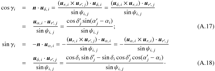 Similarly,
 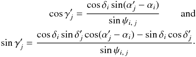 (A.19)Let
  (A.20)(≈n × ur′,j since Mi and are close): vector t is a unit vector tangent in Mi to the minor arc of great circle going from Mi to . Project the sphere on the plane (Mi,t,n) tangent to the sphere in Mi (the specific projection does not matter since we consider only K′-sources in the neighborhood of Mi). We have
  (A.21)and the basis (t,n) is obtained from (ua,ub) by a (β + γ − ß/2)-counterclockwise rotation around + ur, so,
 ![\appendix \setcounter{section}{1} \begin{eqnarray} (\Gamma_i)_{(\vec t,\,\vec n)} &=& \transpose{\Rot}(\beta_i+\gamma_i-\piup/2) \!\cdot\! \Diag\left(a_i^2, b_i^2\right) \! \cdot\! \Rot(\beta_i+\gamma_i-\piup/2), ~~~~~~~~~~~~~~~~~~~~~~~~~~~~ \\ (\Gammapj)_{(\vec t,\,\vec n)} &=& \transpose{\Rot}(\betapj+\gammapj-\piup/2)\! \cdot\! \Diag\left(a_{\smash[t]{j}}'^2, b_{\smash[t]{j}}'^2\right) \! \cdot\! \Rot(\betapj+\gammapj\!-\!\piup/2).~~~~~~~~~~~~~~~~~~~~~~~~~~~~ \end{eqnarray}](/articles/aa/full_html/2014/06/aa20021-12/aa20021-12-eq561.png)
Appendix A.2.2: Case of unknown positional uncertainties
If the positional uncertainty on Mi is unknown, we may model it with (Γi)(t,n) = σ2 Diag(1,1), using the same σ for all K-sources, and derive an estimate of  by maximizing the likelihood to observe the distribution of K- and K′-sources (see Sects. 3.2 and 4.2). For a galaxy, however, the positional uncertainty on its center is likely to increase with its size. If the position angle θi (counted eastward from the north) and the major and minor diameters Di and di of the best-fitting ellipse of some isophote are known for Mi (for instance, parameters PA, D25 and d25 := D25/R25 taken from the RC3 catalog (de Vaucouleurs et al. 1991) or HyperLeda (Paturel et al. 2003)), we may model the positional uncertainty with
 ![\appendix \setcounter{section}{1} \begin{eqnarray} (\Gamma_i)_{(\vec t,\,\vec n)} &=& \transpose{\Rot}(\theta_i+\gamma_i-\piup/2) \cdot \Diag\left(\sigma^2 + [\nu\multspace D_i]^2, \sigma^2 + [\nu\multspace d_i]^2\right) \notag \\&&\quad\cdot \Rot(\theta_i+\gamma_i-\piup/2) \notag \\ &=& \sigma^2\multspace \Diag(1, 1) + \nu^2\multspace \transpose{\Rot}(\theta_i+\gamma_i-\piup/2) \notag \\&&\quad\cdot \Diag\left(D_i^2, d_i^2\right) \cdot \Rot(\theta_i+\gamma_i-\piup/2), \end{eqnarray}](/articles/aa/full_html/2014/06/aa20021-12/aa20021-12-eq571.png) (A.24)and derive estimates of and
(A.24)and derive estimates of and  from the likelihood. Such a technique might indeed be used to estimate the accuracy of coordinates in some catalog (see Paturel & Petit 1999 for another method).
If the positional uncertainty on is unknown too, we can also put 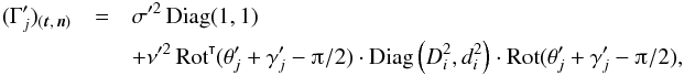 (A.25)with the same σ′ and ν′ for all K′-sources. As
  , only estimates of
  and
and  may be obtained 12 by maximizing the likelihood, not the values of σ, σ′, ν or ν′ themselves.
Appendix A.2.3: Possibly different true positions
A similar technique can be applied if the true centers of K-sources and of their counterparts in K′ sometimes differ. This might be useful in particular when associating galaxies from an optical catalog and from a ultraviolet or far-infrared one, because, while the optical is dominated by smoothly-distributed evolved stellar populations, the ultraviolet and the far-infrared mainly trace star-forming regions. Observations of galaxies (e.g., Kuchinski et al. 2000) have indeed shown that galaxies are very patchy in the ultraviolet, and the same has been observed in the far-infrared.
Since the angular distance between the true centers should increase with the size of the galaxy, we might model this as 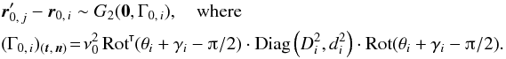 (A.26)We then have
  (A.27)
Once again, if σ, σ′, ν, ν′ and ν0 are unknown, only and  may be estimated through likelihood maximization.
All Figures
|
Fig. 1 One-to-one simulations for f = 1/2, |
| In the text | |
|
Fig. 2 Mean value of different estimators |
| In the text | |
|
Fig. 3 Contour lines of Ls:o (solid) and Lo:o (dashed) in the |
| In the text | |
|
Fig. 4 Contour lines of Ls:o (solid) and Lo:o (dashed) in the |
| In the text | |
|
Fig. 5 Normalized average maximum value |
| In the text | |
Current usage metrics show cumulative count of Article Views (full-text article views including HTML views, PDF and ePub downloads, according to the available data) and Abstracts Views on Vision4Press platform.
Data correspond to usage on the plateform after 2015. The current usage metrics is available 48-96 hours after online publication and is updated daily on week days.
Initial download of the metrics may take a while.