| Issue |
A&A
Volume 565, May 2014
|
|
|---|---|---|
| Article Number | A65 | |
| Number of page(s) | 5 | |
| Section | Interstellar and circumstellar matter | |
| DOI | https://doi.org/10.1051/0004-6361/201322743 | |
| Published online | 12 May 2014 | |
Formation of large-scale magnetic structures associated with the Fermi bubbles
1
Max-Planck-Institut für Kernphysik,
Saupfercheckweg 1,
69117
Heidelberg,
Germany
e-mail:
This email address is being protected from spambots. You need JavaScript enabled to view it.
2
Space Research Institute RAS, 84/32 Profsoyuznaya Street, Moscow
117997,
Russia
3
Astrophysical Big Bang Laboratory, RIKEN, 351-0198
Saitama,
Japan
4
Departament d’Astronomia i Meteorologia, Institut de Ciències del
Cosmos (ICC), Universitat de Barcelona (IEEC-UB), Martí i Franquès 1, 08028
Barcelona,
Spain
e-mail:
This email address is being protected from spambots. You need JavaScript enabled to view it.
Received:
24
September
2013
Accepted:
26
November
2013
Abstract
Context. The Fermi bubbles are part of a complex region of the Milky Way. This region presents broadband extended non-thermal radiation, apparently coming from a physical structure rooted at the Galactic centre and with a partly ordered magnetic field threading it.
Aims. We explore the possibility of an explosive origin for the Fermi bubble region to explain its morphology, in particular that of the large-scale magnetic fields, and provide context for the broadband non-thermal radiation.
Methods. We performed 3D magnetohydrodynamical simulations of an explosion that occurred a few million years ago that pushed and sheared a surrounding magnetic loop, anchored in the molecular torus around the Galactic centre.
Results. Our results can explain the formation of the large-scale magnetic structure in the Fermi bubble region. Consecutive explosive events may match the morphology of the region better. Faster velocities at the top of the shocks than at their sides may explain the hardening with distance from the Galactic plane found in the GeV emission.
Conclusions. In the framework of our scenario, we estimate the lifetime of the Fermi bubbles as ≈2 × 10⁶ yr, with a total energy injected in the explosion(s) of ≳1055 ergs. The broadband non-thermal radiation from the region may be explained by leptonic emission, which is more extended in radio and X-rays, and is confined to the Fermi bubbles in gamma rays.
Key words: shock waves / methods: numerical / Galaxy: center
© ESO, 2014
1. Introduction
Originating in the Galactic centre and extending up to a distance of ≈15 kpc from the Galactic plane, there is a large bipolar structure with counterparts in different wavelengths, from radio to gamma rays. This structure was seen for the first time by ROSAT in X-rays (Snowden et al. 1997). An overlapping extended source was also detected in radio by WMAP (Finkbeiner 2004), and a few years later Fermidetected a somewhat smaller structure in the GeV range, the Fermi bubbles, with a height of ≈8 kpc (Su et al. 2010). A hint of an extension of the GeV emission beyond the Fermi bubbles was also found on scales similar to those of the ROSAT emission (Ackermann et al. 2012). S-PASS (Carretti et al. 2013) and WMAP (Jones et al. 2012) detected a large-scale, partly ordered magnetic-field structure placed at 20°−50° from the Galactic plane in the Fermibubble region, which is larger than the bubbles themselves.
The origin of the Fermi bubbles is still under debate. There are two main hypotheses, which were already discussed in Su et al. (2010): active galactic nucleus (AGN) activity, or a bipolar galactic wind. In fact, a combined origin of central accretion activity and a galactic wind fed by star formation may be possible, as discussed in Carretti et al. (2013). In that work, the authors adopted a leptonic scenario for the Fermi bubbles emission, whereas Crocker & Aharonian (2011) considered hadronic radiation.
Numerical simulations of the dynamics of the Fermi bubbles can be useful to unveil the relevant physical processes underlying the detected radiation. In this regard, numerical hydrodynamical simulations of the Fermi bubbles were performed in 2D by Guo & Mathews (2012) and Guo et al. (2012) and 3D by Yang et al. (2012). In the latter paper, the authors took into account anisotropic diffusion of cosmic rays to explain the sharp edges of the Fermi bubbles in gamma rays. In Guo & Mathews (2012), the X-rays detected by ROSAT were explained as thermal radiation from the surrounding medium heated by a shock, and the gamma rays from the Fermi bubbles as coming from relativistic electrons in the ejecta.
Motivated in particular by the recent detection of a partly-ordered magnetic-field structure in the Fermibubble region, we here present the results of 3D magnetohydrodynamical (MHD) simulations of the structures associated with the Fermi bubbles in the framework of a mini-AGN event in which material is ejected from the central Galactic black hole (see Bland-Hawthorn et al. 2013, for recent observational support for the AGN scenario). We interpret in this context the recent observational findings in radio, in particular concerning the large-scale magnetic field, and suggest a non-thermal nature for the X-ray radiation detected by ROSAT, which is produced by electrons accelerated in the shock driven by the ejecta in the surrounding medium. The GeV emission from the Fermi bubbles might result from particle acceleration in the shock wave of a second explosive event in a recurrent-activity scenario, or particle acceleration within the ejecta, in which shocks, turbulence, and suitable conditions for magnetic reconnection are present. Throughout, we adopted the notation Ab = A/10b, where A has cgs units.
2. Physical scenario
We present an MHD model for the formation of the large-scale magnetic-field structure in the Fermibubble region in the context of accretion-driven explosive events. The evolution and observational properties of the Fermi bubbles and accompanying structures can be strongly influenced by the presence of this large-scale magnetic field.
We assumed that the very central region of the Galaxy is surrounded by a rotating gaseous torus or disc with outer radius RD, effective thickness or inner radius of the torus rD, and rotation speed υD. Loops of magnetic field thread the central region. These magnetic loops, of strength Bl, are anchored in the disc and surround the central region, as shown in Fig. 1.
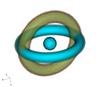 |
Fig. 1 Sketch of the initial configuration: the opaque horizontal torus is a gaseous disc with the distance from the centre of the tube to the centre of the torus RD = 1 kpc and the radius of the tube rD = 0.2 kpc; the translucent vertical ring is a magnetic loop with the same radius and thickness as that of the gaseous disc. The central sphere of radius rs = 0.2 kpc represents a central region with high pressure and velocity: the ejection region. |
In this scenario, the formation of the Fermibubble region proceeds as follows: a molecular disc, with a lifetime ~107 years (Molinari et al. 2011), surrounds the Galactic centre. A magnetic-field loop anchored in the disc also crosses the disc polar regions. At a given time, and possibly episodically, the accretion rate in the central black hole increases dramatically because of for instance the capture of a molecular cloud. Such an accretion event can launch a powerful outflow in the polar direction, as occurs in AGN. The ejecta will stretch the magnetic-field loops that cross the polar regions, and push the external medium up- and sidewards, shocking it. Simultaneously, the external layers of the whole structure, where the ejecta and the external medium are in contact, will be twisted by the rotating gaseous disc through the surrounding magnetic field anchored in the disc and will also be sheared by differential rotation. As shown below, this scenario can produce the partly ordered magnetic-field structure similar to that found in S-PASS.
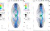 |
Fig. 2 Distribution of the gas velocity modulus and the magnetic-field lines for two models: on the left panel, Etot = 3 × 1055 erg at a time t = 2.3 Myr; on the right panel, Etot = 1055 erg at t = 3.4 Myr. The velocity is presented in units of 108 cm/s and the magnetic-field strength (shown in colour) in units of 400 μG. |
3. Simulations
The simulations presented here were implemented in 3D Cartesian geometry using the PLUTO code (Mignone et al. 2007, 2012), the piece-parabolic method (PPM, Colella & Woodward 1984; Mignone et al. 2005), an HLLD Riemann solver (Miyoshi & Kusano 2008), and applying AMR using the Chombo code (Colella et al. 2009). The flow was approximated as an ideal, adiabatic gas with a magnetic field, one-particle species, and a polytropic index of 5/3. The adopted resolution was 48 × 48 × 96 cells and three levels of AMR, which gives an effective resolution of 384 × 384 × 768 cells. The size of the domain was x ∈ [0,18 kpc], y ∈ [0,18 kpc], and z ∈ [0,36 kpc]. The calculations were carried out in the Moscow State University cluster Chebyshev. The visualization of the results were arranged with VisIt.
3.1. Initial setup
In the centre of our galaxy there is a massive gaseous disc of ~3 × 10⁷ M⊙, a radius of 100 pc, and a rotation speed ~80 km s-1 (see Molinari et al. 2011). The initial configuration of the simulation sets an horizontal gaseous torus in the plane XY (the disc), and a vertical magnetic-field loop in the plane XZ. The torus radius and effective thickness were taken to be RD = 1 kpc and rD = 0.2 kpc, respectively. We fix the central particle density of the torus to 103 cm-3, and assumed constant angular momentum and hydrostatic equilibrium to determine the torus pressure and temperature distribution. We used a truncated Keplerian gravitational potential φ ∝ 1/max(r,0.6 kpc). This potential will not significantly influence the calculation results because the speed of the shock wave at all radii is significantly higher than the escape velocity. The magnetic-loop radius and thickness were taken to be equal to those of the torus (see Fig. 1). The initial strength of the magnetic field in the loop was 100 μG, similar to the observed value in the Galactic centre (Crocker et al. 2010, 2011). Numerical limitations led us to adopt a larger size of the disc/torus and the associated magnetic loop. This also implied that the disc was simulated to be rotating in the gravitational potential of the central region with a rather high speed, υD = 800 km s-1, to obtain a disc angular velocity equal to the actual angular velocity of the molecular disc in the centre of the Galaxy. Hence, in practice, the main difference between our simulation and a more realistic setup is the width of the inner ejection region, which is expected to have a minor impact on the long-term evolution of the simulated structures. In addition, the somewhat unrealistic torus properties do not allow a precise, quantitative comparison between the simulated magnetic-field strength and the observed values. However, given that the magnetic field is not dynamically relevant, it is determined by the fluid evolution, and the obtained global field geometry is expected to be reliable. The lifetime of the central engine activity was assumed to be much shorter than that of the disc or the dynamical scale of the simulation.
The explosive activity produces an axial outflow from a central sphere of radius
rs =
0.2 kpc. The outflow, initially confined to this sphere, was set with
two different total energies for one simulation with one ejection: Etot =
1055 and 3 ×
1055 erg; a particle density of 1 cm-3, and a velocity of
 cm s-1 at ejection,
which is directed along the Z-axis. The gas density of the surrounding medium was
set as in Miller & Bregman (2013):
cm s-1 at ejection,
which is directed along the Z-axis. The gas density of the surrounding medium was
set as in Miller & Bregman (2013):
![Mathematical equation: \hbox{$ n_{\rm bg}=\frac{n_0}{ \left[1\,+\,(R/R_{\rm C})^2 \,+\,(z/z_{\rm C})^2 \right]^{3\beta/2} }, $}](/articles/aa/full_html/2014/05/aa22743-13/aa22743-13-eq41.png) where
n0 =
0.46 cm-3, R is the cylindrical radius, z the distance from the
Galactic plane, and β =
0.71, RC = 0.42 kpc and zC = 0.26 pc are
normalizing constants. The temperature of this medium was fixed to 1.2 × 10⁶ K. Assuming that
accretion events may be recurrent, we performed an additional simulation with two active
episodes. An amount of energy Etot = 1055 erg was now
injected twice, at t =
0 and at t
= 2.5 Myr. The central engine activity was taken to be shorter than the
flow-crossing time, rs/ve ~
104 yr. Because they are much shorter than any relevant
dynamical process in the simulation, the activity periods can indeed be considered as
discrete events. Note that the formation timescale of this magnetic field structure is
~100 pc / 80 km
s-1 ≈ 1 Myr,
which implies that the magnetic loop can continue to be generated between events.
where
n0 =
0.46 cm-3, R is the cylindrical radius, z the distance from the
Galactic plane, and β =
0.71, RC = 0.42 kpc and zC = 0.26 pc are
normalizing constants. The temperature of this medium was fixed to 1.2 × 10⁶ K. Assuming that
accretion events may be recurrent, we performed an additional simulation with two active
episodes. An amount of energy Etot = 1055 erg was now
injected twice, at t =
0 and at t
= 2.5 Myr. The central engine activity was taken to be shorter than the
flow-crossing time, rs/ve ~
104 yr. Because they are much shorter than any relevant
dynamical process in the simulation, the activity periods can indeed be considered as
discrete events. Note that the formation timescale of this magnetic field structure is
~100 pc / 80 km
s-1 ≈ 1 Myr,
which implies that the magnetic loop can continue to be generated between events.
3.2. Results
The distributions of velocity and magnetic-field lines are presented in Fig. 2 for two models, Etot = 3 × 1055 and Etot = 1055 erg, at the time when the size along the Z-direction of the whole structure reached ≈15 kpc. The expansion of the high-pressure region inflates the bubbles and stretches the magnetic-field lines, and meanwhile the rotation of the magnetic-line footpoints twist the magnetic field into a spiral structure. This spiral structure is similar to that observed in Carretti et al. (2013).
The ejected matter from the central engine forms a bipolar, elongated and wide structure. The shock wave travelling through the Galactic halo forms an external bubble of shocked external medium almost as wide as it is long. Surrounded by this shocked external medium, the ejected matter forms a narrower second bubble with its neck at the Galactic centre (see Fig. 3). Covering the inner bubble, at the contact layer between the ejecta and the shocked external medium, the pushed magnetic field is threaded, sheared and anchored in the rotating disc. The magnetic structure induces minor perturbations at the contact layer. In the simulation with two active episodes a second bubble forms inside the first one, as shown in Fig. 4. In this case, the sheared magnetic lines anchored in the molecular disc surround the shock wave formed by the second bubble on the earlier one. An interesting property of the computed solution is the higher speed at the top of the bubble shocks than at their sides. This effect is produced by a decreasing background-density profile.
4. Discussion
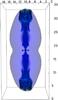 |
Fig. 3 Distribution of the ejected matter tracer (opaque blue-green) and pressure surface (transparent magenta) indicating the position of the shock wave from the model with Etot = 3 × 1055 erg at t = 2.3 Myr. |
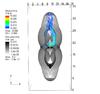 |
Fig. 4 Distribution of the gas pressure (bottom and top) and magnetic-field lines (top) at t = 3.4 Myr for a model with two active episodes, with Etot = 1055 erg each at times t = 0 and t = 2.5 Myr. The pressure is presented in units of 1.67 × 10⁻⁸ pa and the magnetic field (shown in colour) in units of 400 μG. |
We proposed an accretion-ejection, explosive scenario for the formation of the large-scale
magnetic-field structure around the Fermi bubbles. As shown in Fig. 3, one explosion produces very extended ejecta, much larger
than the Fermi bubbles themselves, whose head reaches up to the external
boundary of the whole structure. This mismatch in size may be explained by invoking
acceleration and confinement of the GeV-emitting particles only deep into the ejecta.
Another possibility would come from accretion-ejection events recurring on timescales
≳106 Myr. Such a timescale, and the
energetics derived here, would imply an average injection luminosity of ~1041 erg s-1, compatible with cosmic-ray injection. As shown in Fig.
4, the two-episodes scenario, with this
characteristic timescale and energy budget, nicely reproduces the overall morphology of the
whole Fermibubble region, in particular the sharp edge of the Fermi
bubbles themselves1. It is worth noting that
independently of the simulation, the assumption of a magnetic structure anchored in the
central molecular disc already provides a constraint on the age of the Fermi
bubbles of ≲107 yr. If this were true, such a short lifetime would
disfavour the hadronic scenario. This is so because of the long cooling time of
proton-proton collisions (Kelner et al. 2006):
 yr, ~104 times longer than the dynamical
time of the magnetic field. This low efficiency would require a total energy only in
high-energy protons ~Lγtpp/0.17 = 2 × 1056 ergs, ten times higher than the total
energetics of the Fermi bubbles if they are related to the large-scale
magnetic-field structure, as assumed here. Accounting for dynamical constraints, that is, to
explain the growth of the structure in the surrounding medium on the timescales considered
here, one derives an estimate on the luminosity injected into the Fermi
bubbles of ~1041 ergs. This is ~103 times higher than the energy required to explain the
gamma-ray luminosity, which means that the energy budget is not tight when considering a
leptonic origin of the gamma-ray emission.
yr, ~104 times longer than the dynamical
time of the magnetic field. This low efficiency would require a total energy only in
high-energy protons ~Lγtpp/0.17 = 2 × 1056 ergs, ten times higher than the total
energetics of the Fermi bubbles if they are related to the large-scale
magnetic-field structure, as assumed here. Accounting for dynamical constraints, that is, to
explain the growth of the structure in the surrounding medium on the timescales considered
here, one derives an estimate on the luminosity injected into the Fermi
bubbles of ~1041 ergs. This is ~103 times higher than the energy required to explain the
gamma-ray luminosity, which means that the energy budget is not tight when considering a
leptonic origin of the gamma-ray emission.
We now briefly consider a framework for the broadband detected radiation. Electrons and protons can be accelerated at the shock produced by the ejected matter in the surrounding medium. As just argued, protons are disfavoured by the relatively short timescales involved in the adopted scenario. For electrons, on the other hand, this is not a problem, with the most efficient radiation process at low energies being synchrotron, and at high energies, inverse Compton (IC) with soft Galactic photons of ~1 eV. The maximum energy of the photons produced via synchrotron from shock-accelerated electrons can be estimated as ϵs ≈ 0.12(υs,8)2 η-1 keV (Aharonian & Atoyan 1999), where υs is the forward-shock speed. However, given the slow steepening with energy above ϵs of the synchrotron spectrum of shock-accelerated electrons (Zirakashvili & Aharonian 2007), the effective maximum energy of the synchrotron photons can be estimated to be about 10 × ϵs. With a speed of the shock wave of ~2 × 108 cm s-1, synchrotron X-rays can reach up to few keV. This synchrotron radiation might be able to explain the X-ray shell or arch found by ROSAT (Snowden et al. 1997), which would then have a non-thermal origin instead of a thermal one (both possibilities were discussed for instance); IC emission from the same electrons might explain the hint of GeV radiation found on similar scales (see Fig. 6 in Ackermann et al. 2012). A diffuse lower-energy electron population, extended also beyond the Fermi bubbles, but partially embedded in the spiral-like magnetic lines, might explain the WMAP extended source. The Fermi bubbles themselves would have an IC origin. They would remain confined to the fresher material of the most recent episode, or alternatively, to deeper regions of the whole region if only one explosion took place, as was discussed by Guo & Mathews (2012). A hardening of the GeV radiation along the Z-direction has been observed for the Fermi bubbles (Hooper & Slatyer 2013). This hardening might be explained by the varying speed of the bubble shocks mentioned in Sect. 3.2, affecting (at least slightly) the slope of the distribution of the GeV emitting particles. This hardening might also be consistent with a stronger shock at the top of the bubbles than at their sides.
This explanation for the sharp edge of the Fermi bubbles is only valid as long as the bubbles and the structures at larger scales have a common origin.
Acknowledgments
We thank the anonymous referee for useful and constructive comments. The calculations were carried out in the cluster of Moscow State University Chebyshev. We thank Andrea Mignone and the PLUTO team for the possibility to use the PLUTO code. We also thank the Chombo team for the possibility to use the Chombo code. We would like to thank the VisIt visualization packet team. B.M.V. acknowledges partial support by RFBR grant 12-02-01336-a. V.B-R. acknowledges support by DGI of the Spanish Ministerio de Economía y Competitividad (MINECO) under grants AYA2010-21782-C03-01 and FPA2010-22056-C06-02. V.B-R. acknowledges financial support from MINECO through a Ramón y Cajal fellowship. This research has been supported by the Marie Curie Career Integration Grant 321520.
References
- Ackermann, M., Ajello, M., Atwood, W. B., et al. 2012, ApJ, 750, 3 [NASA ADS] [CrossRef] [Google Scholar]
- Aharonian, F. A., & Atoyan, A. M. 1999, A&A, 351, 330 [NASA ADS] [Google Scholar]
- Bland-Hawthorn, J., Maloney, P., Sutherland, R., & Madsen, G. 2013, ApJ, 778, 58 [NASA ADS] [CrossRef] [Google Scholar]
- Carretti, E., Crocker, R. M., Staveley-Smith, L., et al. 2013, Nature, 493, 66 [NASA ADS] [CrossRef] [PubMed] [Google Scholar]
- Colella, P., Graves, D. T., Keen, N. D., et al. 2009, Chombo Software Package for AMR Applications Design Document, https://seesar.lbl.gov/anag/chombo/ChomboDesign-3.1.pdf [Google Scholar]
- Colella, P., & Woodward, P. R. 1984, J. Comp. Phys., 54, 174 [Google Scholar]
- Crocker, R. M., & Aharonian, F. 2011, Phys. Rev. Lett., 106, 101102 [NASA ADS] [CrossRef] [PubMed] [Google Scholar]
- Crocker, R. M., Jones, D. I., Melia, F., Ott, J., & Protheroe, R. J. 2010, Nature, 463, 65 [NASA ADS] [CrossRef] [Google Scholar]
- Crocker, R. M., Jones, D. I., Aharonian, F., et al. 2011, MNRAS, 413, 763 [NASA ADS] [CrossRef] [Google Scholar]
- Finkbeiner, D. P. 2004, ApJ, 614, 186 [NASA ADS] [CrossRef] [Google Scholar]
- Guo, F., & Mathews, W. G. 2012, ApJ, 756, 181 [NASA ADS] [CrossRef] [Google Scholar]
- Guo, F., Mathews, W. G., Dobler, G., & Oh, S. P. 2012, ApJ, 756, 182 [NASA ADS] [CrossRef] [Google Scholar]
- Hooper, D., & Slatyer, T. R. 2013, in Physics of the Dark Universe, 2, 118 [Google Scholar]
- Jones, D. I., Crocker, R. M., Reich, W., Ott, J., & Aharonian, F. A. 2012, ApJ, 747, L12 [NASA ADS] [CrossRef] [Google Scholar]
- Kelner, S. R., Aharonian, F. A., & Bugayov, V. V. 2006, Phys. Rev. D, 74, 034018 [NASA ADS] [CrossRef] [Google Scholar]
- Mignone, A., Plewa, T., & Bodo, G. 2005, ApJS, 160, 199 [NASA ADS] [CrossRef] [Google Scholar]
- Mignone, A., Bodo, G., Massaglia, S., et al. 2007, ApJS, 170, 228 [Google Scholar]
- Mignone, A., Zanni, C., Tzeferacos, P., et al. 2012, ApJS, 198, 7 [Google Scholar]
- Miller, M. J., & Bregman, J. N. 2013, ApJ, 770, 118 [NASA ADS] [CrossRef] [Google Scholar]
- Miyoshi, T., & Kusano, K. 2008, in Numerical Modeling of Space Plasma Flows, eds. N. V. Pogorelov, E. Audit, & G. P. Zank, ASP Conf. Ser., 385, 279 [Google Scholar]
- Molinari, S., Bally, J., Noriega-Crespo, A., et al. 2011, ApJ, 735, L33 [NASA ADS] [CrossRef] [Google Scholar]
- Snowden, S. L., Egger, R., Freyberg, M. J., et al. 1997, ApJ, 485, 125 [NASA ADS] [CrossRef] [Google Scholar]
- Su, M., Slatyer, T. R., & Finkbeiner, D. P. 2010, ApJ, 724, 1044 [NASA ADS] [CrossRef] [Google Scholar]
- Yang, H.-Y. K., Ruszkowski, M., Ricker, P. M., Zweibel, E., & Lee, D. 2012, ApJ, 761, 185 [NASA ADS] [CrossRef] [Google Scholar]
- Zirakashvili, V. N., & Aharonian, F. 2007, A&A, 465, 695 [NASA ADS] [CrossRef] [EDP Sciences] [Google Scholar]
All Figures
|
Fig. 1 Sketch of the initial configuration: the opaque horizontal torus is a gaseous disc with the distance from the centre of the tube to the centre of the torus RD = 1 kpc and the radius of the tube rD = 0.2 kpc; the translucent vertical ring is a magnetic loop with the same radius and thickness as that of the gaseous disc. The central sphere of radius rs = 0.2 kpc represents a central region with high pressure and velocity: the ejection region. |
| In the text | |
|
Fig. 2 Distribution of the gas velocity modulus and the magnetic-field lines for two models: on the left panel, Etot = 3 × 1055 erg at a time t = 2.3 Myr; on the right panel, Etot = 1055 erg at t = 3.4 Myr. The velocity is presented in units of 108 cm/s and the magnetic-field strength (shown in colour) in units of 400 μG. |
| In the text | |
|
Fig. 3 Distribution of the ejected matter tracer (opaque blue-green) and pressure surface (transparent magenta) indicating the position of the shock wave from the model with Etot = 3 × 1055 erg at t = 2.3 Myr. |
| In the text | |
|
Fig. 4 Distribution of the gas pressure (bottom and top) and magnetic-field lines (top) at t = 3.4 Myr for a model with two active episodes, with Etot = 1055 erg each at times t = 0 and t = 2.5 Myr. The pressure is presented in units of 1.67 × 10⁻⁸ pa and the magnetic field (shown in colour) in units of 400 μG. |
| In the text | |
Current usage metrics show cumulative count of Article Views (full-text article views including HTML views, PDF and ePub downloads, according to the available data) and Abstracts Views on Vision4Press platform.
Data correspond to usage on the plateform after 2015. The current usage metrics is available 48-96 hours after online publication and is updated daily on week days.
Initial download of the metrics may take a while.