| Issue |
A&A
Volume 565, May 2014
|
|
|---|---|---|
| Article Number | A47 | |
| Number of page(s) | 10 | |
| Section | Stellar structure and evolution | |
| DOI | https://doi.org/10.1051/0004-6361/201321830 | |
| Published online | 05 May 2014 | |
Impact of rotation on stochastic excitation of gravity and gravito-inertial waves in stars
1 Laboratoire AIM, CEA/DSM − CNRS − Université Paris Diderot, IRFU/SAp Centre de Saclay, 91191 Gif-sur-Yvette, France
e-mail: This email address is being protected from spambots. You need JavaScript enabled to view it.
2 LESIA, Observatoire de Paris, CNRS UMR 8109, UPMC, Univ. Paris-Diderot, 5 place Jules Janssen, 92195 Meudon, France
e-mail: This email address is being protected from spambots. You need JavaScript enabled to view it.
Received: 4 May 2013
Accepted: 24 March 2014
Abstract
Context. Gravity waves (or their signatures) are detected in stars thanks to helio- and asteroseismology, and they may play an important role in the evolution of stellar angular momentum. Moreover, a previous observational study of the CoRoT target HD 51452 demonstrated the potential strong impact of rotation on the stochastic excitation of gravito-inertial waves in stellar interiors.
Aims. Our goal is to explore and unravel the action of rotation on the stochastic excitation of gravity and gravito-inertial waves in stars.
Methods. The dynamics of gravito-inertial waves in stellar interiors in both radiation and in convection zones is described with a local non-traditional f-plane model. The coupling of these waves with convective turbulent flows, which leads to their stochastic excitation, is studied in this framework.
Results. First, we find that in the super-inertial regime in which the wave frequency is twice as high as the rotation frequency (σ > 2Ω), the evanescence of gravito-inertial waves in convective regions decreases with decreasing wave frequency. Next, in the sub-inertial regime (σ < 2Ω), gravito-inertial waves become purely propagative inertial waves in convection zones. Simultaneously, turbulence in convective regions is modified by rotation. Indeed, the turbulent energy cascade towards small scales is slowed down, and in the case of rapid rotation, strongly anisotropic turbulent flows are obtained that can be understood as complex non-linear triadic interactions of propagative inertial waves. These different behaviours, due to the action of the Coriolis acceleration, strongly modify the wave coupling with turbulent flows. On one hand, turbulence weakly influenced by rotation is coupled with evanescent gravito-inertial waves. On the other hand, rapidly rotating turbulence is intrinsically and strongly coupled with sub-inertial waves. Finally, to study these mechanisms, the traditional approximation cannot be assumed because it does not properly treat the coupling between gravity and inertial waves in the sub-inertial regime.
Conclusions. Our results demonstrate the action of rotation on stochastic excitation of gravity waves thanks to the Coriolis acceleration, which modifies their dynamics in rapidly rotating stars and turbulent flows. As the ratio 2Ω/σ increases, the couplings and thus the amplitude of stochastic gravity waves are amplified.
Key words: hydrodynamics / waves / turbulence / stars: rotation / stars: evolution
Nguyet Tran Minh passed away on January 11, 2013.
© ESO, 2014
1. Introduction
Gravity waves propagate in stably stratified stellar radiation zones, such as the radiative core of low-mass stars and the external radiative envelope of intermediate-mass and massive stars (e.g. Aerts et al. 2010). When such waves (or their signatures) are detected by means of helioseismology (Garcia et al. 2007) and asteroseismology (e.g. Beck et al. 2011; Pápics et al. 2012; Neiner et al. 2012), they constitute a powerful probe of stellar structure (e.g. Turck-Chièze & Couvidat 2011; Bedding et al. 2011) and internal dynamics, for example of differential rotation (Garcia et al. 2007; Beck et al. 2012; Deheuvels et al. 2012; Mosser et al. 2012). Furthermore, when they propagate, gravity waves are able to transport and deposit a net amount of angular momentum because of their radiative damping and corotation resonances (e.g. Goldreich & Nicholson 1989; Schatzman 1993; Zahn et al. 1997). Therefore, they are invoked, together with magnetic torques, to explain the quasi-uniform rotation until 0.2 R⊙ in the solar radiative core (Charbonnel & Talon 2005), the mixing of light elements in low-mass stars (Talon & Charbonnel 2005), the weak differential rotation in subgiant and red giant stars (Ceillier et al. 2012), and the transport of angular momentum necessary to explain mass-loss in active massive stars such as Be stars (Huat et al. 2009; Neiner et al. 2013; Lee & Saio 1993; Lee 2013). Thus, it is necessary to understand their excitation mechanisms well and precisely predict their amplitude.
In single stars, two mechanisms can excite gravity waves: the κ-mechanism due to opacity bumps (e.g. Unno et al. 1989; Gastine & Dintrans 2008) and stochastic motions in both the bulk of convective regions and at their interfaces with adjacent radiation zones where turbulent convective structures (plumes) penetrate because of their inertia (e.g. Press 1981; Browning et al. 2004; Rogers & Glatzmaier 2005; Belkacem et al. 2009b; Cantiello et al. 2009; Samadi et al. 2010; Brun et al. 2011; Rogers et al. 2012; Shiode et al. 2013; Alvan et al. 2014). In this work, we focus on stochastic excitation.
In addition to stochastically excited mixed gravito-acoustic modes that are currently detected with space asteroseismology, for example in red giants (e.g. Beck et al. 2011), a detection has been obtained with CoRoT in the hot Be star HD 51452 (Neiner et al. 2012). In this star, which rotates close to its critical angular velocity, we discovered gravity modes that are strongly influenced by the Coriolis acceleration that are gravito-inertial modes (Dintrans & Rieutord 2000; Mathis 2009; Ballot et al. 2010). It was proposed that these modes are probably excited stochastically by turbulent convection in the core or/and in the subsurface convection zone, since this star is too hot to excite gravity modes with the κ-mechanism. Moreover, the detected gravito-inertial modes with the largest amplitudes have frequencies below the inertial one at 2Ω (where Ω is the angular velocity of the star), which are those most influenced by the Coriolis acceleration. Therefore, this discovery points out the potentially important action of rotation on stochatic excitation of gravity and gravito-inertial waves (GIWs) in stellar interiors. This has been little explored until now (Belkacem et al. 2009a; Rogers et al. 2013).
To identify the associated mechanisms and unravel the related signatures, we choose here to generalise the work by Goldreich & Kumar (1990) and Lecoanet & Quataert (2013) taking the action of the Coriolis acceleration into account. First, in Sect. 2, we present the local rotating set-up in which we describe the different regimes of the dynamics of GIWs in both radiation and convection zones. Next, we study in Sect. 3 their stochastic excitation by turbulent convective flows with particular attention on the effects of slow and rapid rotation. Finally, in Sect. 4, we conclude on the impact of rotation on the stochastic excitation of GIWs in stars and discuss the consequences for asteroseismology and for studying their angular momentum evolution.
2. Gravito-inertial waves in stellar interiors
The first step to explore the impact of rotation on GIWs stochastic excitation in stellar interiors is to describe properly their different propagation regimes as a function of their frequencies.
2.1. Rotating “f-plane” reference frame
To reach our objective, we followed the local approach adopted by Goldreich & Kumar (1990) and Lecoanet & Quataert (2013), but taking rotation into account. We therefore considered a Cartesian region, centred on a point M of a radiation-convection interface, where Θ is the angle between the local effective gravity geff1 and the rotation vector Ω (see Fig. 1). Mx, My, and Mz are the axes along the local azimuthal, latitudinal, and vertical (along geff) directions. We define zc, the altitude of the transition between the radiation and convection zones. This so-called f-plane (Pedlosky 1982) is co-rotating with the stellar angular velocity Ω. To write equations of wave dynamics in this reference frame, we then introduce the two components of this vector  (1)along the vertical and latitudinal directions, respectively. Following Gerkema & Shrira (2005), both components are taken into account to ensure a complete and correct treatment of the GIWs dynamics in the radiation and convective regions. Assuming constant f gives the so-called non-traditional f-plane, contrary to the usual traditional approximation in which the horizontal component
  is neglected (Eckart 1961). Taking
  into account allows one to correctly treat the coupling between GIWs and inertial waves (Gerkema et al. 2008).
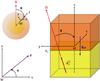 |
Fig. 1 Local studied f-plane reference frame( is the unit-vector along the rotation axis). Here, the radiative and convective regions are plotted in yellow and orange. This configuration corresponds to the case of low-mass stars; zc is the altitude of the transition radiation/convection. The vertical structure of this set-up can be inverted to treat the case of intermediate-mass and massive stars. |
2.2. Poincaré equation
To obtain the equation that governs the GIWs dynamics, the Poincaré equation, we write the linearised equations of motion of the stellar stratified fluid on the non-traditional f-plane assuming the Boussinesq and the Cowling approximations (Gerkema & Shrira 2005; Cowling 1941). First, we introduce the GIWs’ velocity field u = (u,v,w), where u, v and w are the components in the local azimuthal, latitudinal, and vertical directions. Next, we define the fluid buoyancy  (2)and the corresponding Brunt-Väisälä frequency
  (3)where ρ′ and
  are the density fluctuation and the reference background density, and t is the time. The three linearised components of the momentum equation are given by
  (4)Next, we write the continuity equation in the Boussinesq approximation
 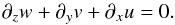 (5)Finally, we get the equation for energy conservation in the adiabatic limit
 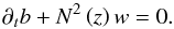 (6)Eliminating the horizontal components of the velocity, the pressure and the buoyancy, we reduce the system to an equation for the vertical velocity
 ![Mathematical equation: \begin{equation} \partial_{t,t}\left[{\nabla}^{2} w\right]+4\left({\vec\Omega}\cdot{\vec\nabla}\right)^{2}w+N^2{\nabla}_{\rm H}^{2}w=0, \label{M1} \end{equation}](/articles/aa/full_html/2014/05/aa21830-13/aa21830-13-eq33.png) (7)where
(7)where  is the horizontal Laplacian. We then consider a given monochromatic GIW with a frequency σ that propagates in the direction (cosα,sinα) in the (Mxy) plane (see Fig. 1). Introducing the reduced horizontal coordinate χ = xcosα + ysinα (with ∂x = cosα∂χ and ∂y = sinα∂χ) and substituting
 ![Mathematical equation: \hbox{$w\left(\vec r,t\right)=W\left(\vec r\right)\exp\left[{\rm i}\sigma\,t\right]$}](/articles/aa/full_html/2014/05/aa21830-13/aa21830-13-eq40.png) , we finally obtain the Poincaré equation for GIWs:
, we finally obtain the Poincaré equation for GIWs:  (8)where
  (9)Moreover, even if the GIWs dynamics constitutes a bidimensionnal problem because of the mixed derivative ∂χ,z (e.g. Dintrans & Rieutord 2000), it is possible in our set-up to introduce the transformation
 ![Mathematical equation: \begin{equation} W=\Psi\left(z\right)\exp\left[{\rm i} k_{\perp}\left(\chi+{\tilde\delta} z\right)\right]\hbox{ }\hbox{ }\hbox{where}\hbox{ }\hbox{ }{\tilde\delta}=-\frac{B}{C}, \label{vert} \end{equation}](/articles/aa/full_html/2014/05/aa21830-13/aa21830-13-eq44.png) (10)that leads to
(10)that leads to  (11)where
 ![Mathematical equation: \begin{equation} k_{V}^{2}\left(z\right)=k_{\perp}^2\left[\frac{B^2-AC}{C^2}\right]=k_{\perp}^2\left[\frac{N^2\left(z\right)-\sigma^2}{\sigma^2-f^2}+\left(\frac{\sigma\,f_{\rm s}}{\sigma^2-f^2}\right)^2\right], \label{M3} \end{equation}](/articles/aa/full_html/2014/05/aa21830-13/aa21830-13-eq46.png) (12)k⊥ being the wave number in the χ direction (Gerkema & Shrira 2005). This enables us to use the method of vertical modes as in the non-rotating case and the associated tools since, as demonstrated in Gerkema & Shrira (2005), the modal functions Wj that verify boundary conditions constitute an orthogonal and complete basis.
(12)k⊥ being the wave number in the χ direction (Gerkema & Shrira 2005). This enables us to use the method of vertical modes as in the non-rotating case and the associated tools since, as demonstrated in Gerkema & Shrira (2005), the modal functions Wj that verify boundary conditions constitute an orthogonal and complete basis.
2.3. Gravito-inertial wave propagation in rotating stars
We now describe the GIWs propagation as a function of their frequency σ.
At a given z, GIWs are propagative if Δ = B2 − AC> 0. This leads to an allowed frequency spectrum σ−<σ<σ+, where ![Mathematical equation: \begin{equation} \sigma_{\pm}=\frac{1}{\sqrt 2}\sqrt{\left[N^2+f^2+f_{s}^{2}\right]\pm\sqrt{\left[N^2+f^2+f_{s}^{2}\right]^{2}-\left(2fN\right)^{2}}}. \end{equation}](/articles/aa/full_html/2014/05/aa21830-13/aa21830-13-eq53.png) (13)In convective regions, which excite GIWs, the local vertical wave number (Eq. (12)) becomes
(13)In convective regions, which excite GIWs, the local vertical wave number (Eq. (12)) becomes ![Mathematical equation: \begin{equation} k^{2}_{\rm CZ}\equiv k_{\perp}^2\frac{\sigma^2}{\left(\sigma^2-f^2\right)^2}\left[\left(f^2+f_{s}^{2}\right)-\sigma^2\right]=k_{\perp}^{2}\frac{\left[\left[{{\widetilde R}_{\rm o}}\left(\Theta,\alpha\right)\right]^{-2}-1\right]}{\left(1-R_{\rm o}^{-2}\cos^2\Theta\right)^{2}}, \label{M4} \end{equation}](/articles/aa/full_html/2014/05/aa21830-13/aa21830-13-eq54.png) (14)where we defined a local wave Rossby number
(14)where we defined a local wave Rossby number ![Mathematical equation: \begin{equation} {\widetilde R}_{\rm o}=R_{\rm o}\left[\cos^{2}\Theta+\sin^{2}\alpha\sin^{2}\Theta\right]^{-1/2} \end{equation}](/articles/aa/full_html/2014/05/aa21830-13/aa21830-13-eq55.png) (15)expressed as a function of the wave’s Rossby number Ro = σ/ 2Ω.
(15)expressed as a function of the wave’s Rossby number Ro = σ/ 2Ω.
Then, we identify for α = π/ 2 the allowed frequency domain for inertial waves 0 <σ< 2Ω (i.e. Ro< 1). On one hand, in the local super-inertial regime ( ), there are turning points (zt;i) in the radiation zones for which
  (see Eq. (16)) and GIWs are evanescent in convection zones. On the other hand, in the local sub-inertial domain (
 ), GIWs propagate in the whole radiation zone and become propagative inertial waves in convection zones.
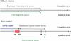 |
Fig. 2 Low-frequency spectrum of waves in a non-rotating (Ω = 0, top) and in a rotating (bottom) star. For each case, waves in the convection and radiation zones are indicated at the top and bottom. The red box corresponds to sub-inertial gravito-inertial waves where the cavities of gravity and inertial waves are coupled. |
These two behaviours (see Fig. 2) have been isolated by Dintrans & Rieutord (2000) for a 1.5 M⊙ star (see their Fig. 6). The cases of typical solar-type stars (1 M⊙) and massive stars (12 M⊙) are illustrated in Fig. 3 for a small horizontal cross-section box along a given radius. By defining a synthetic profile of positive Brunt-Vaïsälä frequency with a maximum value Nmax computed using a 1D stellar evolution code, we plot {σ−,σ+} profiles for various values of the rotation rate: Ω = 0.1Ωc (in blue), 0.5Ωc (in purple) and Ωc (in red). The critical angular velocity is  , where G, M and R are the gravity universal constant, the stellar mass, and radius, respectively. For the 12 M⊙ massive star, we filtered out the bumps of N at the top of the convective core and just below the stellar surface. We point out that SΩ = Nmax/ 2Ω(andSΩ;c = Nmax/ 2Ωc) are the control parameters that determine whether the second regime, in which GIWs propagate in the whole radiation zone and become inertial waves in the convection zone, spreads over a wide frequency range. As shown in Fig. 3, this can be the case of rapidly rotating massive stars. Therefore, we distinguish these two regimes from now.
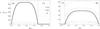 |
Fig. 3 Synthetic profiles of {σ−,σ+} (color lines) and N (solid black line) in μHz for a 1 M⊙ solar-type star (left) and a 12 M⊙ massive star (right) for α = π/ 2, Θ = 5π/ 12, and various rotation rates: Ω = 0.1Ωc (blue dotted-dashed line), 0.5Ωc (green dashed line), 1Ωc (red long-dashed line). The border between the convection and radiation zones (CZ and RZ) is given by the grey vertical line. For the 12 M⊙ massive star, we filtered out the bumps of N at the top of the convective core and just below the stellar surface. In convection zones, σ− ~ N ~ 0. |
2.3.1. Super-inertial regime 
There are two turning points (zt;1, zt;2 with zt;1<zt;2) in the radiation zone in the super-inertial regime for which  that corresponds to values of z where
 ![Mathematical equation: \begin{equation} N^2=\sigma^2\frac{\left[\sigma^2-\left(f^2+f_{s}^{2}\right)\right]}{\left(\sigma^2-f^2\right)}\cdot \label{TP} \end{equation}](/articles/aa/full_html/2014/05/aa21830-13/aa21830-13-eq89.png) (16)To derive an asymptotic expression of Ψ (defined in Eq. (10)) in the whole radiation zone, we went beyond the usual JWKB approximation (Fröman & Fröman 2005), which fails at turning points, and adopted the uniform Airy approximation (Berry & Mount 1972). The latter has been introduced in quantum mechanics and allows us to derive asymptotic expressions in terms of Airy functions, which are valid close and far from turning points. Following Brault et al. (1988), we obtain for an external convective zone
(16)To derive an asymptotic expression of Ψ (defined in Eq. (10)) in the whole radiation zone, we went beyond the usual JWKB approximation (Fröman & Fröman 2005), which fails at turning points, and adopted the uniform Airy approximation (Berry & Mount 1972). The latter has been introduced in quantum mechanics and allows us to derive asymptotic expressions in terms of Airy functions, which are valid close and far from turning points. Following Brault et al. (1988), we obtain for an external convective zone ![Mathematical equation: \begin{equation} \Psi\left(z<z_{\rm c}\right)=A\left(\frac{\Phi\left(z\right)}{k_{V}^{2}\left(r\right)}\right)^{1/4}{\rm Ai}\left[\Phi\left(z\right)\right], \end{equation}](/articles/aa/full_html/2014/05/aa21830-13/aa21830-13-eq91.png) (17)where
(17)where  (18)and kV given in Eq. (12). In the convective region, GIWs are evanescent, and we obtain using the asymptotic properties of Airy functions and Eq. (14)
 ![Mathematical equation: \begin{equation} \Psi\left(z>z_{\rm c}\right)=\frac{A}{\sqrt{k_{\perp}{p}}}\exp\left[-k_{\perp}{p}\left(z-z_{\rm c}\right)-\Delta\left(z_{t;2},z_{\rm c}\right)\right], \end{equation}](/articles/aa/full_html/2014/05/aa21830-13/aa21830-13-eq94.png) (19)where we define
(19)where we define  (20)We recall that zc is the altitude of the transition radiation/convection. In this regime, p corresponds to the decay rate of the velocity in the convection zone. If we verify no-slip boundary conditions w(zb,χ,t) = w(zs,χ,t) = 0,where zb and zs are the altitudes corresponding to the bottom and the top of the box, we can deduce eigenfrequencies using Bohr quantisation (Landau & Lifshitz 1965)
  , where k is an integer.
Then, the complete bidimensionnal expression for the vertical velocity is obtained using Eq. (10): ![Mathematical equation: \begin{eqnarray} W\left(z>z_{\rm c},\chi\right)&=&\frac{A}{\sqrt{k_{\perp}{p}}}\exp\left[-k_{\perp}{p}\left(R_{\rm o}\right)\left(z-z_{\rm c}\right)-\Delta\left(z_{t;2},z_{\rm c}\right)\right]\nonumber\\ &&\times\cos\left[k_{\perp}\left(\chi+{\tilde\delta}\left(R_{\rm o}\right)z\right)\right], \label{bidisuper} \end{eqnarray}](/articles/aa/full_html/2014/05/aa21830-13/aa21830-13-eq102.png) (21)where
(21)where  (22)The evolution of p and
  as a function of Ro and Θ are plotted in Fig. 4. In the super-inertial regime, p increases with Ro (with p → 1 for Ro → ∞). This means that the decay rate of the wave function in the convective zone decreases when the rotation rate increases until Ro = 1. Moreover, tends to vanish at large Ro while it increases with the rotation rate until Ro = 1. This corresponds to the fact that, as soon as rotation becomes important, the problem is non-separable in z and χ while it is completely separable in the non-rotating case (i.e. Ro → ∞). Accordingly, modifications of GIW velocity fields occur. This shows the important impact of the Coriolis acceleration, which will modify their couplings with convective flows.
We used the uniform Airy approximation. For a of very steep transition from convection to radiation on a characteristic distance d such that k⊥d< 1, Lecoanet & Quataert (2013) pointed that it would be better to adopt solutions of Eq. (11) corresponding to a buoyancy frequency profile expressed as a function of an hyperbolic tangent. This combination of steep transition and rotation will be examined in the near future and is beyond the scope of this work. In fact, the evanescent or propagative behaviours of GIWs in convection zones only depend on the sign of  .
.
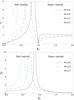 |
Fig. 4 Evolution of p (top) and |
2.3.2. Sub-inertial regime 
For the sub-inertial regime, waves propagate in the whole domain without any turning point ( ). Assuming the JWKB approximation in the radiation zone, we can write
  (23)where kV is given in Eq. (12). In the convective region, we derive for inertial waves using Eq. (14):
 ![Mathematical equation: \begin{equation} \Psi\left(z>z_{\rm c}\right)=\frac{A}{\sqrt{k_{\perp}p}}\sin\left[k_{\perp}p\left(z-z_{\rm c}\right)+\Delta\left(z_{\rm b},z_{\rm c}\right)\right], \end{equation}](/articles/aa/full_html/2014/05/aa21830-13/aa21830-13-eq120.png) (24)where p and Δ have been defined in Eq. (20). As in the super-inertial case, we can use Bohr quantisation to obtain eigenfrequencies in the case of no-slip boundary conditions, that is
(24)where p and Δ have been defined in Eq. (20). As in the super-inertial case, we can use Bohr quantisation to obtain eigenfrequencies in the case of no-slip boundary conditions, that is  , where n is an integer.
The complete bidimensionnal expression for the vertical velocity is obtained using Eq. (10): ![Mathematical equation: \begin{eqnarray} W\left(z>z_{\rm c},\chi\right)&=&\frac{A}{\sqrt{k_{\perp}{p}}}\sin\left[k_{\perp}p\left(R_{\rm o}\right)\left(z-z_{\rm c}\right)+\Delta\left(z_{\rm b},z_{\rm c}\right)\right]\nonumber\\ &&\times\cos\left[k_{\perp}\left(\chi+{\tilde\delta}\left(R_{\rm o}\right)z\right)\right]. \label{bidisub} \end{eqnarray}](/articles/aa/full_html/2014/05/aa21830-13/aa21830-13-eq124.png) (25)In this regime, p (see Eq. (20)) is the vertical wave number of the propagative inertial wave in the convection zone. The variations of p and as a function of Ro in the sub-inertial regime, shown in Fig. 4, imply that the velocity field becomes more and more oscillatory as the rotation rate increases until Ro = cos(Θ), where the denominators of p and vanish.
(25)In this regime, p (see Eq. (20)) is the vertical wave number of the propagative inertial wave in the convection zone. The variations of p and as a function of Ro in the sub-inertial regime, shown in Fig. 4, imply that the velocity field becomes more and more oscillatory as the rotation rate increases until Ro = cos(Θ), where the denominators of p and vanish.  corresponds to the critical colatitude above which GIWs are trapped in the radiation zone in the sub-inertial regime (e.g. Mathis & de Brye 2012). This behaviour is strongly different from the one obtained in the super-inertial regime and will modify the GIWs stochastic excitation by convective flows, as represented in Fig. 5.
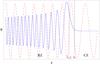 |
Fig. 5 Cartoon for the general behaviours of Ψ in the super-inertial (solid blue line) and in the sub-inertial (red dashed line) regimes around the external turning point zt;2 (vertical purple line) for a star with a convective envelope (for z>zc). The border between the convection and radiation zones (CZ and RZ) is given by the black vertical line. |
3. Gravito-inertial wave stochastic excitation by turbulent convection
3.1. Forced Poincaré equation
To obtain the amplitude of GIWs excited by turbulent convective zones, we followed Goldreich & Kumar (1990) and Lecoanet & Quataert (2013). The equation for the vertical component of the wave velocity (w) is given for the radiation zone in Eq. (7) and for the convective region by ![Mathematical equation: \begin{equation} \partial_{t,t}\left[\nabla^{2}w\right]+4\left({\vec\Omega}\cdot{\vec\nabla}\right)^{2}w=\partial_{t}{\mathcal S}=\partial_{t}\left[\partial_{z}{\vec\nabla}\cdot{\vec F}-\nabla^{2}F_{z}\right]. \label{InH} \end{equation}](/articles/aa/full_html/2014/05/aa21830-13/aa21830-13-eq128.png) (26)We introduce the turbulent source function
(26)We introduce the turbulent source function  , defined as a function of the convective Reynolds stresses
  . A complete overview of the different excitation sources that can excite GIWs in a rotating star has been given in Belkacem et al. (2009a, see also Samadi & Goupil 2001). They demonstrated that we can focus on this term
  .
.
Using the orthogonality of GIW functions in our Cartesian set-up, which has been demonstrated by Gerkema & Shrira (2005), we can derive a formal expression for the amplitude of GIWs depending on their super- or sub-inertial behaviour. Following Goldreich & Kumar (1990) and Lecoanet & Quataert (2013), we expand the solution of Eq. (26) as  (27)where σi are the eigenfrequencies, Wi the corresponding eigenfunctions of the homogeneous equation, and
  is the horizontal cross-section of the box. We obtain
 ![Mathematical equation: \begin{eqnarray} \left| A_{\hbox{sup}}\right|&=&\frac{\sqrt {\mathcal A}\left|\sigma^2-f^2\right|}{2 \sigma\ k_{\perp}^{2}}\frac{1}{\left|\mathcal C\right|}\nonumber\\ &&\times\frac{1}{\sqrt{k_{\perp}{p}}}\int_{-\infty}^{\,t}{\rm d}\tau \int_{\mathcal V}{\rm d}x\,{\rm d}y\,{\rm d}{\zeta}\,\partial_{t}{\mathcal S}\left(x,y,\zeta,\tau\right)\nonumber\\ &&\times \exp\left[-{\rm i}\,k_{\perp}\left[\left(x\cos\alpha+y\sin\alpha\right)+{\tilde\delta}\left(R_{\rm o}\right)\zeta\right]-{\rm i}\sigma\tau\right]\nonumber\\ &&\times \exp\left[-k_{\perp}{p\left(R_{\rm o}\right)}\left(\zeta-z_{\rm c}\right)-\Delta\left(z_{t;2},z_{\rm c}\right)\right] \label{FA1} \end{eqnarray}](/articles/aa/full_html/2014/05/aa21830-13/aa21830-13-eq136.png) (28)and
(28)and ![Mathematical equation: \begin{eqnarray} \left| A_{\hbox{sub}}\right|&=&\frac{\sqrt {\mathcal A}\left|\sigma^2-f^2\right|}{2 \sigma\ k_{\perp}^{2}}\frac{1}{\left|\mathcal C\right|}\nonumber\\ &&\times \frac{1}{\sqrt{k_{\perp}{p}}}\int_{-\infty}^{\,t}{\rm d}\tau \int_{\mathcal V}{\rm d}x\,{\rm d}y\,{\rm d}{\zeta}\,\partial_{t}{\mathcal S}\left(x,y,\zeta,\tau\right)\nonumber\\ &&\times \exp\left[-{\rm i}\,k_{\perp}\left[\left(x\cos\alpha+y\sin\alpha\right)+{\tilde\delta}\left(R_{\rm o}\right)\zeta\right]-{\rm i}\sigma\tau\right]\nonumber\\ &&\times \sin\left[k_{\perp}p\left(R_{\rm o}\right)\left(\zeta-z_{\rm c}\right)+\Delta\left(z_{\rm b},z_{\rm c}\right)\right], \label{FA2} \end{eqnarray}](/articles/aa/full_html/2014/05/aa21830-13/aa21830-13-eq137.png) (29)where
(29)where  is the volume of the box. The normalisation coefficient (Gerkema & Shrira 2005)
 ![Mathematical equation: \begin{equation} {\mathcal C}\equiv\left[\int{\rm d}\chi\int_{z_{\rm b}}^{z_{\rm s}}\left[N^{2}\left(z\right)-R^2\left(z\right)\right]W_{i}\left(z,\chi\right)W_{i}^{*}\left(z,\chi\right){\rm d}z\right], \end{equation}](/articles/aa/full_html/2014/05/aa21830-13/aa21830-13-eq139.png) (30)where
(30)where  (31)is introduced because the eigenfunctions Wi are only orthogonal. Applying Eqs. (28)−(29) to the non-rotating case and working with the vertical displacement ξz, where w = ∂tξz, we recover Eq. (C3) in Lecoanet & Quataert (2013). These formal expressions demonstrate that the coupling between the wave’s velocity and convective turbulence is a function of Ro = σ/ 2Ω (via p, see Eq. (20), and δ, see Eq. (22)). In the super-inertial regime, turbulent convective flows are correlated with an evanescent gravito-inertial wave (the last exponential term), while in the sub-inertial regime they couple with a propagative inertial wave (the sinusoidal term). To proceed, we have to be more specific on the turbulent source function, and to discuss its modification by rotation.
3.2. Modification of turbulence by rotation
3.2.1. Various regimes
Rotation strongly modifies the properties of turbulent flows. First, it induces anisotropy of the flows with a tendency to a bi-dimensionalisation. Next, the turbulent energy cascade towards small scales is slowed down, in particular in the case of decaying turbulence. Finally, relatively strong columnar structures along the direction of the axis of rotation appear.
We consider the non-linear Navier-Stockes equation in the rotating reference frame for an homogeneous fluid:  (32)where b corresponds to the buoyancy. If we introduce the characteristic scales of velocity (U), length (L) and time (T) tonon-dimensionalised Eq. (32), we obtain
 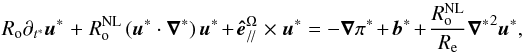 (33)where t∗ = t/T, ∇∗ = L∇, u∗ = u/U, π∗ = P/ (ρ2ΩLU), b∗ = b/ (2ΩU) and is the unit vector along the rotation axis (
 is respectively the perpendicular one). We have introduced the linear and non-linear Rossby numbers and the Reynoldsnumber
 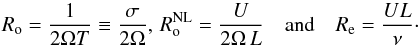 (34)Then, neglecting the buoyancy force, different regimes can be identified.
-
When Ro<< 1,
 and Re>> 1, we identify the geostrophic equilibrium between theCoriolis acceleration and the pressure gradient.
 -
When Ro ≤ 1 and
, we obtain linear progressive inertial waves, superimposed on the geostrophic equilibrium state. -
When
 and Re>> 1, we obtain the so-called wave turbulence regime, where the rotating strongly anisotropic turbulent flow can be described as a system of inertial waves in interaction. In this regime, thanks to non-linearities, transfers of energy occur between the various scales of the flow.
 -
When
 and Re>> 1, we recover the case of the “classical” turbulence perturbed by rotation, with a characteristic time-scale that is longer than or of the order of the turbulent convective turnover time L/U. The turbulent flows are close to the assumption of homogeneous and isotropic turbulence if
  . Finally, turbulence is coupled to super-inertial GIWs (Ro> 1) that are evanescent in convection zones.
In stellar convection zones, characteristic dimensionless numbers can be qualitatively evaluated using the scaling-law for the convective velocities proposed by Brun (2014) ![Mathematical equation: \begin{equation} u_{\rm c}\approx\left[\frac{L_{*}}{{\overline \rho}_{\rm CZ}R^{2}}\right]^{1/3}, \label{Vc} \end{equation}](/articles/aa/full_html/2014/05/aa21830-13/aa21830-13-eq167.png) (35)where L∗ is the luminosity of the star, R its radius and
(35)where L∗ is the luminosity of the star, R its radius and  the mean density of the studied convective region. Then, the convective Rossby number can be evaluated as
 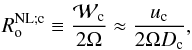 (36)where
  is the convective vorticity and Dc the thickness of the convective zone.
3.2.2. Asymptotic case of slow rotation
We consider the regime with discussed above, where rotation only weakly affects turbulence. This regime has been previously studied in the literature (Samadi & Goupil 2001; Samadi et al. 2003a,b; Belkacem et al. 2009a; Samadi et al. 2010). We followed the method of Samadi & Goupil (2001) and Samadi et al. (2003a,b, 2010), and introduce the volumetric excitation rate, which is obtained from an integration by part of Eq. (28): ![Mathematical equation: \begin{equation} {\mathcal P}_{\rm R}=\frac{\pi^3}{I}\int_{0}^{M}{\rm d}m\left\{\,F_{\rm kin}\, L_{\rm c}^{4}\int_{0}^{\infty}\, \frac{{\rm d}k}{k^2}\left[\frac{16}{15} \left(\frac{{\rm d}^{2}W}{{\rm d}z^{2}}\right)^{2}{\tilde{\mathcal S}}\left(k,\sigma\right)\right]\right\}, \label{Pf} \end{equation}](/articles/aa/full_html/2014/05/aa21830-13/aa21830-13-eq173.png) (37)where
(37)where ![Mathematical equation: \begin{equation} {\tilde{\mathcal S}}\left(k,\sigma\right)=w_{\rm c}^{-3}L_{\rm c}^{-4}\left[E\left(k\right)\right]^{2}G_{k}\left(\sigma\right). \label{Pf-in} \end{equation}](/articles/aa/full_html/2014/05/aa21830-13/aa21830-13-eq174.png) (38)In these equations, wc is the rms value of the vertical component of the convective velocity uc,
(38)In these equations, wc is the rms value of the vertical component of the convective velocity uc,  the vertical flux of kinetic energy, Lc the characteristic length of convective flows, dm the infinitesimal mass element, and I the mass-mode. Moreover,
  is the kinetic energy spectrum associated with the turbulent convective velocity field, where k is the eddy wavenumber in the Fourier space, and
  describes the time-dependent part of the turbulent spectrum, which models the correlation time-scale of an eddy with a wavenumber k. As pointed out by Samadi (2011), the separation between turbulent velocities and waves and this expansion of the turbulent source function can only be applied to isotropic turbulence in the regime of slow rotation, and we show in Sect. 3.2.3 that they must be abandoned for rapid rotation. For a quantitative estimate of the amplitude, E and Gk can be computed using 3D numerical simulations (e.g. Samadi et al. 2003a; Belkacem et al. 2009b; Rogers et al. 2013).
Until Sect. 3.2, the action of rotation has been taken into account for the modification of waves’ velocity field alone. In particular, we have demonstrated that super-inertial GIWs are less and less evanescent when their Rossby number (Ro) is decreased. This increases the possibility of couplings between GIWs and turbulent eddies. In fact, the weaker  for a wave, the stronger the possibility for its coupling with an eddy of characteristic length-scale 1 /k⊥. In Eq. (37), we introduced wc, the rms value of the vertical component of the convective velocity (Eq. (35)). However, while it provides us the strength of the vertical flux of kinetic energy transported by convective flows, it does not take their modification by rotation into account. We therefore considered the evolution of the kinetic energy spatial spectrum () as a function of the non-linear Rossby number (
 ). Indeed, while in the non-rotating case, we can approximate the spectrum using a Kolmogorov-like form
  , it becomes steeper as soon as rotation is increased:
  (see e.g. Zhou 1995; Morize et al. 2005). Therefore, it is necessary to obtain spectra of rotating turbulent flows using numerical simulations and laboratory experiments to take into account the action of the Coriolis acceleration on convective flows.
The rate of energy injection in GIWs is also a function of their time-correlation with turbulent eddies (Samadi et al. 2010). On one hand, it is highest for P = 2π/σ ≥ Tc, where Tc is the characteristic eddy turn-over time and P is the period of the modes. On the other hand, it decreases strongly when P<Tc. Since rotation affects general properties of turbulent eddies, it will also affect the time-correlation function.
To evaluate how turbulent convective flows are influenced by rotation, we can use results obtained in numerical simulations and laboratory experiments. We introduce the Rayleigh number, Ra = αTgΔTD3/κν, which compares the strength of buoyancy and diffusion in convective regions, and the Ekman number, E = ν/ 2ΩD2, which compares the viscous force and the Coriolis acceleration. αT is the fluid’s thermal expansion coefficient, g the gravity, ΔT the temperature difference across the convective region, and D its thickness. ν and κ are the fluid viscous and thermal diffusivities, respectively. King et al. (2012) and Julien et al. (2012a) showed that the control parameter of the problem is a transition Rayleigh number that scales as a power-law of the Ekman number, that is Ra;t ~ Eγ (Julien et al. 2012a gives γ = −8/5, while King et al. 2012 predicted γ = −3/2). At a given rotation rate, if Ra>Ra;t, the convection is weakly modified by rotation, while cases where Ra<Ra;t are in the rapidly rotating regime. A complete discussion of the properties of the flows can be found in King et al. (2013; see also Julien et al. 2012b).
The modification of the amplitude of super-inertial GIWs in the slowly rotating case thus results from the modification of their propagation in convection zones by the Coriolis acceleration (Sect. 2.3) and of its impact on convective eddies.
3.2.3. Asymptotic case of rapid rotation
In the case of rapid rotation, as explained in Sect. 3.2.1, we cannot separate turbulence from propagative inertial waves (which correspond to sub-inertial GIWs in the radiation zones). Indeed, turbulent flows, which become highly anisotropic, can be understood as non-linearly interacting inertial waves. Following Sen et al. (2012; see also e.g. Smith & Waleffe 1999; Galtier 2003; Cambon et al. 2004; Bourouiba et al. 2012), we introduce the wave-vector expansion 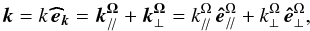 (39)which has been decomposed along the directions respectively parallel and orthogonal to the rotation axis. Note that for α = π/ 2 (see Fig. 1), we have
  (40)which corresponds to and for the inertial waves described in Sect. 2.3.2. Then, the general solution for the velocity field (u) of propagative inertial waves in the convection zone can be expanded (see Smith & Waleffe 1999):
 ![Mathematical equation: \begin{equation} {\vec u}\left(\vec x,t\right)=\sum_{\vec k,s}b_{s}\left(\vec k\right){\vec h}_{s}\left(\vec k\right)\exp\left[{\rm i}\left(\vec k\cdot\vec x-\sigma_{s}\,t\right)\right], \label{v_rapid} \end{equation}](/articles/aa/full_html/2014/05/aa21830-13/aa21830-13-eq211.png) (41)where
(41)where  (42)is the Craya-Herring helical basis and
  (43)Waves are circularly polarised and propagate with velocities that are normal to k and rotate around it during their propagation with a group velocity vg = sk × (2Ω × k)/ | k | 3. Waves with a negative helicity (s = 1) propagate upward (vg·Ω> 0), while those with a positive helicity (s = −1) travel downward (vg·Ω< 0).
If we adopt the framework of the weak inertial-wave turbulence theory (e.g. Galtier 2003), we substitute Eq. (41) in Eq. (32), which leads to the following equation for bs(k) ≡ bsk: ![Mathematical equation: \begin{eqnarray} \left(\partial_{t}+\nu\, {\vec k}^{2} \right)b_{s_k}=R_{\rm o}^{\rm NL}\sum_{{\vec k}+{\vec p}+{\vec q}\,=\,0}^{\sigma_{s_k}+\sigma_{s_p}+\sigma_{s_q}\,=\,0}\sum_{s_p,s_q}\left\{C_{{\vec k},{\vec p},{\vec q}}^{{s_k},{s_p},{s_q}}b_{s_p}^{*}b_{s_q}^{*}\right.\nonumber\\ {\left.\times\exp\left[{\rm i}\left(\sigma_{s_k}+\sigma_{s_p}+\sigma_{s_q}\right)t\right] \right\}}, \end{eqnarray}](/articles/aa/full_html/2014/05/aa21830-13/aa21830-13-eq221.png) (44)with
(44)with ![Mathematical equation: \begin{equation} C_{{\vec k},{\vec p},{\vec q}}^{s_k,s_p,s_q}=\left(s_q\,q-s_p\,p\right)\left[\left({\vec h}_{s_k}^{*}\times{\vec h}_{s_p}^{*}\right)\cdot{\vec h}_{s_q}^{*}\right], \end{equation}](/articles/aa/full_html/2014/05/aa21830-13/aa21830-13-eq222.png) (45)where ∗ indicates a complex conjugate. The non-linear terms on the right-hand side correspond to triadic interactions and are of the order of . In the rapidly rotating case where is small, the inertial waves oscillate on a rapid time-scale (2Ω)-1 while their amplitudes (bsk) evolve on the slow time-scale
(45)where ∗ indicates a complex conjugate. The non-linear terms on the right-hand side correspond to triadic interactions and are of the order of . In the rapidly rotating case where is small, the inertial waves oscillate on a rapid time-scale (2Ω)-1 while their amplitudes (bsk) evolve on the slow time-scale  . In this framework, the terms
 ![Mathematical equation: \hbox{$\exp\left[{\rm i}\left(\sigma_{s_k}+\sigma_{s_p}+\sigma_{s_q}\right)t\right] $}](/articles/aa/full_html/2014/05/aa21830-13/aa21830-13-eq227.png) with σsk + σsp + σsq ≠ 0 are rapidly oscillating but they average out to zero when one considers the long time-scale of order
with σsk + σsp + σsq ≠ 0 are rapidly oscillating but they average out to zero when one considers the long time-scale of order  . Therefore we only consider near resonance configurations in which
  (46)If we assume the Waleffe instability assumption (Smith & Waleffe 1999), these equations allow us to understand the mechanism of transfer of energy towards 2D vortical modes (with ) that is responsible for the formation of strong columnar flows observed in rapidly rotating fluids in laboratory experiments and in numerical simulations.
However, as pointed out by Sen et al. (2012), it is necessary to go beyond this formalism. Indeed, in realistic flows there are energy transfers from 3D to 2D modes but also from 2D to 3D modes that cannot be described by the weak inertial-wave turbulence theory. Following Sen et al. (2012), we decompose the velocity field in the convective region as a superposition of 3D (or wave modes) and of slow 2D vortical modes:  (47)where
  (48)The total kinetic energy is expanded as
 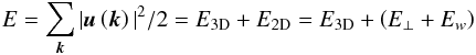 (49)where
  (50)By multiplying the spectral form of the momentum equation by u∗(k), we can derive the two coupled differential equations for the total energy in 3D inertial modes and in 2D slow modes (see Sen et al. 2012):
  (51)In these equations, εj, where j = {3D,2D}, corresponds to the forced energy injection into j-modes and Πj is the energy that is transferred to small scales and dissipated per unit of time, balancing εj. Finally, Π2D → 3D, which is of the order of , is the flux of energy that is transferred from 2D to 3D modes when it is positive (and from 3D to 2D modes when it is negative).
When applied to numerical simulations of rapidly rotating turbulent flows (e.g. Sen et al. 2012), these equations allow us to isolate the energy contained in 3D and in 2D modes and thus their respective strength. Moreover, Mininni et al. (2011) and Sen et al. (2012) tested various types of forcing and demonstrated that in most of their simulations, Π2D → 3D is negative for low values of , which indicates that the energy goes from 3D modes towards 2D ones for larger scales, and positive for high values of (energy is transferred to 3D modes for smaller scales; see also Fig. 12 in Sen et al. 2012). Moreover, to identify wave vectors in rapidly rotating turbulent regions, it is interesting to define the axisymmetric energy spectrum  (52)where θk is the colatitude with respect to the rotation axis in the Fourier space. We identify
 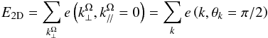 (53)and
 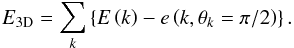 (54)An interesting application of this diagnosis was reported by Clark di Leoni et al. (2014) who examined the strength of inertial waves in a rotating turbulent flow. Moreover, Sen et al. (2013) proposed a weak-wave turbulence theory for rotationally constrained slow inertial waves. For non-helical dynamics, it leads to a spectrum of the form
  (55)which has been observed in several numerical simulations (e.g. Teitelbaum & Mininni 2012; Mininni et al. 2012). In the helical case, the scaling ∝
 isobserved (see also Mininni & Pouquet 2010). This anisotropic kinetic energy spectrum is directly related to the amplitude coefficients of inertial waves (bs(k); see Eqs. (41) and (54)) that become sub-inertial GIWs in the adjacent radiative zone. It corresponds to Eqs. (37) and (38) derived for the slowly rotating case, the important differences being that for rapid rotation, waves and turbulent flows cannot be separated as in the slowly rotating regime and that turbulence becomes anisotropic.
In the context of the stochastic excitation of GIWs in rapidly rotating stars, these diagnoses are very important. First, as we showed in Figs. 3 and 5, 3D inertial modes that propagate in turbulent convection zones convert into sub-inertial GIWs in the adjacent radiative regions. Next, the turbulent structures associated to 2D modes, in which the energy propagates along the rotation axis, will also excite GIWs because of their penetration at the interfaces between convection and radiation (e.g. Takehiro & Lister 2001). In this context, it is mandatory to go beyond the traditional approximation, the non-traditional terms being those that allow us to properly couple the gravity and inertial modes (see Fig. 3).
In the two above subsections, we have discussed the way in which rotation deeply impacts the nature of turbulent flows that stochastically excite GIWs in stellar interiors. On one hand, in the case of slow rotation, turbulence is only weakly perturbed by rotation and is coupled to super-inertial GIWs, which are evanescent in convective zones. When rotation is increased, they are increasingly less evanescent until Ro = 1. On the other hand, in the case of rapidly rotating stars, turbulent flows are deeply modified by rotation and become intrisically coupled with inertial waves, which corresponds to sub-inertial GIWs. This theoretical picture shows the importance of computing high-resolution numerical simulations of rapidly rotating turbulent convective stellar regions with adjacent radiative zones in a near future to test our scenario as a function of Ro and of for various stellar types (e.g. Browning et al. 2004; Ballot et al. 2007; Brown et al. 2008; Matt et al. 2011; Brun et al. 2011; Rogers et al. 2013; Alvan et al. 2013, 2014).
 |
Fig. 6 Wave-turbulence couplings as a function of the non-linear Rossby number |


4. Discussion and conclusions
We have formally demonstrated that rotation, through the Coriolis acceleration, modifies the stochastic excitation of gravity waves and GIWs, the control parameters being the wave’s Rossby number Ro = σ/ 2Ω and the non-linear Rossby number of convective turbulent flows. On one hand, in the super-inertial regime (σ> 2Ω,i.e.Ro> 1), the evanescent behaviour of GIWs above (below) the external (internal) turning point becomes increasingly weaker as the rotation speed grows until Ro = 1. Simultaneously, the turbulent energy cascade towards small scales is slowed down. The coupling between super-inertial GIWs and given turbulent convective flows is then amplified as described in Eq. (28). On the other hand, in the sub-inertial regime (σ< 2Ω,i.e.Ro< 1), GIWs become propagative inertial waves in the convection zone. In the case of rapid rotation, turbulent flows, which become strongly anisotropic, result from their non-linear interactions. Sub-inertial GIWs that correspond to propagating inertial waves in convection zones are then intrinsically and strongly coupled to rapidly rotating turbulence, as discussed in Sect. 3.2.3. These different regimes are summarised in Fig. 6.
These effects are of great interest for asteroseismic studies of rotating stars since gravity wave and GIW amplitudes are thus expected to be stronger in rapidly rotating stars, a conclusion that is supported by recent numerical simulations (Rogers et al. 2013). For example, until recently, stochastically excited gravity waves were thought to be of too low an amplitude to be detected even with space missions such as CoRoT (Samadi et al. 2010). The discovery of stochastically excited GIWs in the rapid rotator HD 51452 (Neiner et al. 2012) proved that such waves can be detected. Our results show that the amplitude of these waves can be enhanced by rotation. The interpretation of observed pulsational frequencies in rapid rotators should take this into account. In particular, oscillations observed in β Cep and slowly pulsating B (SPB) stars should not be systematically attributed to the κ-mechanism, as was done until now, if the star rotates fast. For example, the GIWs observed in HD 43317 (Pápics et al. 2012) might be of stochastic origin and might have been enhanced by rapid rotation. This is of course especially true for Be and Bn stars.
Moreover, the related transport of angular momentum, which until now was believed to become less efficient because of the GIWs equatorial trapping in the sub-inertial regime (Mathis et al. 2008; Mathis 2009; Mathis & de Brye 2012), may be sustained thanks to the stronger stochastic excitation by turbulent convective flows. This may have important consequences for example for rapidly rotating young low-mass stars (Talon & Charbonnel 2008; Charbonnel et al. 2013) and active intermediate-mass and massive stars such as Be stars. For example, Neiner et al. (2013) proposed that the outburst of the Be star HD 49330 observed by CoRoT (Huat et al. 2009) might have been caused by to the deposit of angular momentum by GIWs just below the surface (see also Lee 2013).
Our prediction now needs to be compared with realistic numerical simulations of stochastic excitation of GIWs in stellar interiors (e.g. Brun et al. 2011; Rogers et al. 2012, 2013; Alvan et al. 2013), laboratory experiments (Perrard et al. 2013), and with a larger statistical sample of observed pulsating stars with detected GIWs. Moreover, a global formalism to treat the problem in the spheroidal geometry corresponding to rotating stars must be built in a near future.
This effective gravity is the sum of the self-gravity g and of the centrifugal acceleration 1/2 Ω2∇S2, where S is the distance from the rotation axis.
Acknowledgments
We thank the referee for her/his remarks and suggestions that improved the original manuscript. This work was supported by the French Programme National de Physique Stellaire (PNPS) of CNRS/INSU, the CNES-SOHO/GOLF grant and asteroseismology support at CEA-Saclay, the CNES-CoRoT grant at LESIA, and by the Programme Physique Théorique et ses interfaces of CNRS/INP. Authors are grateful to A.-S. Brun, L. Alvan, R. A. Garcia, T. Rogers, M. Lebars, and D. Lecoanet for fruitful discussions and to P. Eggenberger, T. Decressin and M. Briquet for providing stellar models.
References
- Aerts, C., Christensen-Dalsgaard, J., & Kurtz, D. W. 2010, Asteroseismology, Astron. Astrophys. Lib. (Springer Science + Business Media) [Google Scholar]
- Alvan, L., Brun, A.-S., & Mathis, S. 2013, in SF2A-2013: Proc. of the Annual meeting of the French Society of Astronomy and Astrophysics, eds. L. Cambresy, F. Martins, E. Nuss, & A. Palacios, 77 [Google Scholar]
- Alvan, L., Brun, A. S., & Mathis, S. 2014 [arXiv:1403.4052] [Google Scholar]
- Ballot, J., Brun, A. S., & Turck-Chièze, S. 2007, ApJ, 669, 1190 [Google Scholar]
- Ballot, J., Lignières, F., Reese, D. R., & Rieutord, M. 2010, A&A, 518, A30 [NASA ADS] [CrossRef] [EDP Sciences] [Google Scholar]
- Beck, P. G., Bedding, T. R., Mosser, B., et al. 2011, Science, 332, 205 [NASA ADS] [CrossRef] [PubMed] [Google Scholar]
- Beck, P. G., Montalban, J., Kallinger, T., et al. 2012, Nature, 481, 55 [NASA ADS] [CrossRef] [Google Scholar]
- Bedding, T. R., Mosser, B., Huber, D., et al. 2011, Nature, 471, 608 [NASA ADS] [CrossRef] [PubMed] [Google Scholar]
- Belkacem, K., Mathis, S., Goupil, M. J., & Samadi, R. 2009a, A&A, 508, 345 [NASA ADS] [CrossRef] [EDP Sciences] [Google Scholar]
- Belkacem, K., Samadi, R., Goupil, M. J., et al. 2009b, A&A, 494, 191 [NASA ADS] [CrossRef] [EDP Sciences] [Google Scholar]
- Berry, M. V., & Mount, K. E. 1972, Rep. Prog. Phys., 35, 315 [Google Scholar]
- Bourouiba, L., Straub, D. N., & Waite, M. L. 2012, J. Fluid Mech., 690, 129 [NASA ADS] [CrossRef] [Google Scholar]
- Brault, P., Vallee, O., & Tran Minh, N. 1988, J. Phys. A, 21, L67 [NASA ADS] [CrossRef] [Google Scholar]
- Brown, B. P., Browning, M. K., Brun, A. S., Miesch, M. S., & Toomre, J. 2008, ApJ, 689, 1354 [CrossRef] [Google Scholar]
- Browning, M. K., Brun, A. S., & Toomre, J. 2004, ApJ, 601, 512 [NASA ADS] [CrossRef] [Google Scholar]
- Brun, A. S., Miesch, M. S., & Toomre, J. 2011, ApJ, 742, 79 [NASA ADS] [CrossRef] [Google Scholar]
- Cambon, C., Rubinstein, R., & Godeferd, F. S. 2004, New J. Phys., 6, 73 [NASA ADS] [CrossRef] [Google Scholar]
- Cantiello, M., Langer, N., Brott, I., et al. 2009, A&A, 499, 279 [NASA ADS] [CrossRef] [EDP Sciences] [Google Scholar]
- Ceillier, T., Eggenberger, P., García, R. A., & Mathis, S. 2012, Astron. Nachr., 333, 971 [NASA ADS] [CrossRef] [Google Scholar]
- Charbonnel, C., & Talon, S. 2005, Science, 309, 2189 [NASA ADS] [CrossRef] [PubMed] [Google Scholar]
- Charbonnel, C., Decressin, T., Amard, L., Palacios, A., & Talon, S. 2013, A&A, 554, A40 [NASA ADS] [CrossRef] [EDP Sciences] [Google Scholar]
- Clark di Leoni, P., Cobelli, P. J., Mininni, P. D., Dmitruk, P., & Matthaeus, W. H. 2014, Phys. Fluids, 26, 035106 [NASA ADS] [CrossRef] [Google Scholar]
- Cowling, T. G. 1941, MNRAS, 101, 367 [NASA ADS] [Google Scholar]
- Deheuvels, S., Garcia, R., Chaplin, W. J., et al. 2012, ApJ, 756, 19 [NASA ADS] [CrossRef] [Google Scholar]
- Dintrans, B., & Rieutord, M. 2000, A&A, 354, 86 [NASA ADS] [Google Scholar]
- Eckart, C. 1961, Phys. Fluids, 4, 791 [NASA ADS] [CrossRef] [Google Scholar]
- Fröman, N., & Fröman, P. O. 2005, Physical Problems Solved by the Phase-Integral Method (Cambridge: Cambridge University Press) [Google Scholar]
- Galtier, S. 2003, Phys. Rev. E, 68, 5301 [Google Scholar]
- Garcia, R. A., Turck-Chièze, S., Jiménez-Reyes, S. J., et al. 2007, Science, 316, 1591 [NASA ADS] [CrossRef] [PubMed] [Google Scholar]
- Gastine, T., & Dintrans, B. 2008, A&A, 490, 743 [NASA ADS] [CrossRef] [EDP Sciences] [Google Scholar]
- Gerkema, T., & Shrira, V. I. 2005, J. Fluid Mech., 529, 195 [NASA ADS] [CrossRef] [Google Scholar]
- Gerkema, T., Zimmerman, J. T. F., Maas, L. R. M., & van Haren, H. 2008, Rev. Geophys., 46, 2004 [NASA ADS] [CrossRef] [Google Scholar]
- Goldreich, P., & Kumar, P. 1990, ApJ, 363, 694 [NASA ADS] [CrossRef] [Google Scholar]
- Goldreich, P., & Nicholson, P. D. 1989, ApJ, 342, 1075 [NASA ADS] [CrossRef] [Google Scholar]
- Huat, A.-L., Hubert, A.-M., Baudin, F., et al. 2009, A&A, 506, 95 [NASA ADS] [CrossRef] [EDP Sciences] [Google Scholar]
- Julien, K., Knobloch, E., Rubio, A. M., & Vasil, G. M. 2012a, Phys. Rev. Lett., 109, 4503 [Google Scholar]
- Julien, K., Rubio, A. M., Grooms, I., & Knobloch, E. 2012b, Geophys. Astrophys. Fluid Dynamics, 106, 392 [Google Scholar]
- King, E. M., Stellmach, S., & Aurnou, J. M. 2012, J. Fluid Mech., 691, 568 [NASA ADS] [CrossRef] [Google Scholar]
- King, E. M., Stellmach, S., & Buffett, B. 2013, J. Fluid Mech., 717, 449 [NASA ADS] [CrossRef] [Google Scholar]
- Landau, L. D., & Lifshitz, E. M. 1965, Quantum mechanics (Oxford: Pergamon Press) [Google Scholar]
- Lecoanet, D., & Quataert, E. 2013, MNRAS, 773 [Google Scholar]
- Lee, U. 2013, PASJ, 65, 122 [NASA ADS] [Google Scholar]
- Lee, U., & Saio, H. 1993, MNRAS, 261, 415 [Google Scholar]
- Mathis, S. 2009, A&A, 506, 811 [NASA ADS] [CrossRef] [EDP Sciences] [Google Scholar]
- Mathis, S., & de Brye, N. 2012, A&A, 540, A37 [NASA ADS] [CrossRef] [EDP Sciences] [Google Scholar]
- Mathis, S., Talon, S., Pantillon, F.-P., & Zahn, J.-P. 2008, Sol. Phys., 251, 101 [NASA ADS] [CrossRef] [Google Scholar]
- Matt, S. P., Do Cao, O., Brown, B. P., & Brun, A. S. 2011, Astron. Nachr., 332, 897 [NASA ADS] [CrossRef] [Google Scholar]
- Mininni, P. D., & Pouquet, A. 2010, Phys. Fluids, 22, 035105 [Google Scholar]
- Mininni, P. D., Dmitruk, P., Matthaeus, W. H., & Pouquet, A. 2011, Phys. Rev. E, 83, 016309 [NASA ADS] [CrossRef] [Google Scholar]
- Mininni, P. D., Rosenberg, D., & Pouquet, A. 2012, J. Fluid Mech., 699, 263 [NASA ADS] [CrossRef] [Google Scholar]
- Morize, C., Moisy, F., & Rabaud, M. 2005, Phys. Fluids, 17, 095105 [NASA ADS] [CrossRef] [Google Scholar]
- Mosser, B., Goupil, M. J., Belkacem, K., et al. 2012, A&A, 548, A10 [NASA ADS] [CrossRef] [EDP Sciences] [Google Scholar]
- Neiner, C., Floquet, M., Samadi, R., et al. 2012, A&A, 546, A47 [NASA ADS] [CrossRef] [EDP Sciences] [Google Scholar]
- Neiner, C., Mathis, S., Saio, H., & Lee, U. 2013, in ASP Conf. Ser. 479, eds. H. Shibahashi, & A. E. Lynas-Gray, 319 [Google Scholar]
- Pápics, P. I., Briquet, M., Baglin, A., et al. 2012, A&A, 542, A55 [NASA ADS] [CrossRef] [EDP Sciences] [Google Scholar]
- Pedlosky, J. 1982, Geophysical fluid dynamics (Berlin: Springer-Verlag) [Google Scholar]
- Perrard, S., Le Bars, M., & Le Gal, P. 2013, in Lect. Notes Phys. 865, eds. M. Goupil, K. Belkacem, C. Neiner, F. Lignières, & J. J. Green (Berlin: Springer Verlag), 239 [Google Scholar]
- Press, W. H. 1981, ApJ, 245, 286 [NASA ADS] [CrossRef] [Google Scholar]
- Rogers, T. M., & Glatzmaier, G. A. 2005, MNRAS, 364, 1135 [NASA ADS] [CrossRef] [Google Scholar]
- Rogers, T. M., Lin, D. N. C., & Lau, H. H. B. 2012, ApJ, 758, L6 [NASA ADS] [CrossRef] [Google Scholar]
- Rogers, T. M., Lin, D. N. C., McElwaine, J. N., & Lau, H. H. B. 2013, ApJ, 772, 21 [NASA ADS] [CrossRef] [Google Scholar]
- Samadi, R. 2011, in Lect. Notes Phys. 832 eds. J.-P. Rozelot, & C. Neiner, (Berlin: Springer Verlag), 305 [Google Scholar]
- Samadi, R., & Goupil, M.-J. 2001, A&A, 370, 136 [NASA ADS] [CrossRef] [EDP Sciences] [Google Scholar]
- Samadi, R., Nordlund, Å., Stein, R. F., Goupil, M. J., & Roxburgh, I. 2003a, A&A, 404, 1129 [NASA ADS] [CrossRef] [EDP Sciences] [Google Scholar]
- Samadi, R., Nordlund, Å., Stein, R. F., Goupil, M. J., & Roxburgh, I. 2003b, A&A, 403, 303 [Google Scholar]
- Samadi, R., Belkacem, K., Goupil, M. J., et al. 2010, Ap&SS, 328, 253 [NASA ADS] [CrossRef] [Google Scholar]
- Schatzman, E. 1993, A&A, 279, 431 [NASA ADS] [Google Scholar]
- Sen, A., Mininni, P. D., Rosenberg, D., & Pouquet, A. 2012, Phys. Rev. E, 86, 036319 [NASA ADS] [CrossRef] [Google Scholar]
- Sen, A., Julien, K., & Pouquet, A. 2013 [arXiv:1312.7497] [Google Scholar]
- Shiode, J. H., Quataert, E., Cantiello, M., & Bildsten, L. 2013, MNRAS, 430, 1736 [NASA ADS] [CrossRef] [Google Scholar]
- Smith, L. M., & Waleffe, F. 1999, Phys. Fluids, 11, 1608 [NASA ADS] [CrossRef] [Google Scholar]
- Takehiro, S.-i., & Lister, J. R. 2001, Earth Planet. Sci. Lett., 187, 357 [NASA ADS] [CrossRef] [Google Scholar]
- Talon, S., & Charbonnel, C. 2005, A&A, 440, 981 [NASA ADS] [CrossRef] [EDP Sciences] [Google Scholar]
- Talon, S., & Charbonnel, C. 2008, A&A, 482, 597 [NASA ADS] [CrossRef] [EDP Sciences] [Google Scholar]
- Teitelbaum, T., & Mininni, P. D. 2012, Phys. Rev. E, 86, 6320 [Google Scholar]
- Turck-Chièze, S., & Couvidat, S. 2011, Rep. Prog. Phys., 74, 086901 [NASA ADS] [CrossRef] [Google Scholar]
- Unno, W., Osaki, Y., Ando, H., Saio, H., & Shibahashi, H. 1989, Nonradial oscillations of stars (Tokyo: University of Tokyo Press) [Google Scholar]
- Zahn, J.-P., Talon, S., & Matias, J. 1997, A&A, 322, 320 [Google Scholar]
- Zhou, Y. 1995, Phys. Fluids, 7, 2092 [NASA ADS] [CrossRef] [Google Scholar]
All Figures
|
Fig. 1 Local studied f-plane reference frame( is the unit-vector along the rotation axis). Here, the radiative and convective regions are plotted in yellow and orange. This configuration corresponds to the case of low-mass stars; zc is the altitude of the transition radiation/convection. The vertical structure of this set-up can be inverted to treat the case of intermediate-mass and massive stars. |
| In the text | |
|
Fig. 2 Low-frequency spectrum of waves in a non-rotating (Ω = 0, top) and in a rotating (bottom) star. For each case, waves in the convection and radiation zones are indicated at the top and bottom. The red box corresponds to sub-inertial gravito-inertial waves where the cavities of gravity and inertial waves are coupled. |
| In the text | |
|
Fig. 3 Synthetic profiles of {σ−,σ+} (color lines) and N (solid black line) in μHz for a 1 M⊙ solar-type star (left) and a 12 M⊙ massive star (right) for α = π/ 2, Θ = 5π/ 12, and various rotation rates: Ω = 0.1Ωc (blue dotted-dashed line), 0.5Ωc (green dashed line), 1Ωc (red long-dashed line). The border between the convection and radiation zones (CZ and RZ) is given by the grey vertical line. For the 12 M⊙ massive star, we filtered out the bumps of N at the top of the convective core and just below the stellar surface. In convection zones, σ− ~ N ~ 0. |
| In the text | |
|
Fig. 4 Evolution of p (top) and |
| In the text | |
|
Fig. 5 Cartoon for the general behaviours of Ψ in the super-inertial (solid blue line) and in the sub-inertial (red dashed line) regimes around the external turning point zt;2 (vertical purple line) for a star with a convective envelope (for z>zc). The border between the convection and radiation zones (CZ and RZ) is given by the black vertical line. |
| In the text | |
|
Fig. 6 Wave-turbulence couplings as a function of the non-linear Rossby number |
| In the text | |
Current usage metrics show cumulative count of Article Views (full-text article views including HTML views, PDF and ePub downloads, according to the available data) and Abstracts Views on Vision4Press platform.
Data correspond to usage on the plateform after 2015. The current usage metrics is available 48-96 hours after online publication and is updated daily on week days.
Initial download of the metrics may take a while.