| Issue |
A&A
Volume 564, April 2014
|
|
|---|---|---|
| Article Number | L10 | |
| Number of page(s) | 5 | |
| Section | Letters | |
| DOI | https://doi.org/10.1051/0004-6361/201423490 | |
| Published online | 07 April 2014 | |
B fields in OB stars (BOB): The discovery of a magnetic field in a multiple system in the Trifid nebula, one of the youngest star forming regions⋆
1 Leibniz-Institut für Astrophysik Potsdam (AIP), An der Sternwarte 16, 14482 Potsdam, Germany
e-mail: This email address is being protected from spambots. You need JavaScript enabled to view it.
2 Argelander-Institut für Astronomie, Universität Bonn, Auf dem Hügel 71, 53121 Bonn, Germany
3 Instituto de Ciencias Astronomicas, de la Tierra, y del Espacio (ICATE), 5400 San Juan, Argentina
4 Institute for Astro- and Particle Physics, University of Innsbruck, Technikerstr. 25/8, 6020 Innsbruck, Austria
5 European Southern Observatory, Karl-Schwarzschild-Str. 2, 85748 Garching, Germany
6 Universität Potsdam, Institut für Physik und Astronomie, 14476 Potsdam, Germany
7 Institut d’Astrophysique et de Géophysique, Université de Liège, Allée du 6 Août, Bât. B5c, 4000 Liège, Belgium
8 Main Astronomical Observatory, 27 Academica Zabolotnogo Str., 03680 Kiev, Ukraine
9 Dr. Karl Remeis-Observatory & ECAP, University Erlangen-Nuremberg, Sternwartstr. 7, 96049 Bamberg, Germany
Received: 23 January 2014
Accepted: 25 February 2014
Abstract
Aims. Recent magnetic field surveys in O- and B-type stars revealed that about 10% of the core-hydrogen-burning massive stars host large-scale magnetic fields. The physical origin of these fields is highly debated. To identify and model the physical processes responsible for the generation of magnetic fields in massive stars, it is important to establish whether magnetic massive stars are found in very young star-forming regions or whether they are formed in close interacting binary systems.
Methods. In the framework of our ESO Large Program, we carried out low-resolution spectropolarimetric observations with FORS 2 in 2013 April of the three most massive central stars in the Trifid nebula, HD 164492A, HD 164492C, and HD 164492D. These observations indicated a strong longitudinal magnetic field of about 500–600 G in the poorly studied component HD 164492C. To confirm this detection, we used HARPS in spectropolarimetric mode on two consecutive nights in 2013 June.
Results. Our HARPS observations confirmed the longitudinal magnetic field in HD 164492C. Furthermore, the HARPS observations revealed that HD 164492C cannot be considered as a single star as it possesses one or two companions. The spectral appearance indicates that the primary is most likely of spectral type B1–B1.5 V. Since in both observing nights most spectral lines appear blended, it is currently unclear which components are magnetic. Long-term monitoring using high-resolution spectropolarimetry is necessary to separate the contribution of each component to the magnetic signal. Given the location of the system HD 164492C in one of the youngest star formation regions, this system can be considered as a Rosetta Stone for our understanding of the origin of magnetic fields in massive stars.
Key words: binaries: close / stars: early-type / stars: fundamental parameters / stars: magnetic field / stars: variables: general / stars: individual: HD 164492C
Based on observations obtained in the framework of the ESO Prg. 191.D-0255(A,B).
© ESO, 2014
1. Introduction
Magnetic fields have fundamental effects not only on the evolution of massive stars, on their rotation, and on the structure, dynamics, and heating of their radiatively-driven winds, but also on their final display as supernova or gamma-ray burst. About a few dozen massive magnetic stars are currently known, just enough to establish the fraction of magnetic, core-hydrogen burning stars to be of the order of 8% (Grunhut et al. 2012), which appears to be similar to that of intermediate-mass stars. While it is established that the magnetic fields in massive stars are not dynamo-supported, but stable with decay times exceeding the stellar lifetime, their origin is highly debated. The two main competing ideas are that the fields are either “fossil” remnants of the Galactic ISM field that are amplified during the collapse of a magnetised gas cloud (e.g. Price & Bate 2007), or that they are formed in a dramatic close-binary interaction, i.e., in a merger of two stars or a dynamical mass transfer event (e.g. Ferrario et al. 2009). The intermediate-mass stars show a magnetic fraction during their pre-main sequence evolution similar to Herbig stars (e.g., Hubrig et al. 2009; 2013, and references therein; Alecian et al. 2013) as their main-sequence descendants, which may speak for fossil fields. On the other hand, there are almost no close binaries amongst the magnetic intermediate-mass main-sequence Ap-type stars (e.g. Carrier et al. 2002). Since this is expected if they were merger products, this argues for the binary hypothesis of the field origin.
We present our spectropolarimetric observations of three massive stars in the Trifid nebula in the framework of our “B fields in OB stars” (BOB) collaboration. This nebula is a very young (≲106 yrs) and active site of star formation containing a rich population of young stellar objects (YSOs) and protostars (e.g. Cernicharo et al. 1998). The spectacular, well-known optical H ii region provides an ideal place for investigating the onset of star birth and triggered star formation. This large nebula is ionised by the O7.5 Vz star HD 164492A (Sota et al. 2014), which is the central object of the multiple system ADS 10991, containing at least seven components (A to G; Kohoutek et al. 1999). Due to the faintness of the components HD 164492B and HD 164492E-G (all have visual magnitudes fainter than 10.6), we only searched for a magnetic field for the three most massive components, HD 164492A, C, and D.
2. Magnetic field measurements using FORS 2 spectropolarimetry
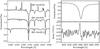 |
Fig. 1 Left panel: Stokes I FORS 2 spectra of three components of the multiple system ADS 10991 (HD 164492A, HD 164492C, and HD 164492D) in the vicinity of the Hγ line. Right panel: Stokes I (top) and V / I (bottom) FORS 2 spectra of HD 164492C in the vicinity of the Hβ line. |
Three components of the system ADS 10991, HD 164492A, C, and D, were observed with the FOcal Reducer low dispersion Spectrograph (FORS 2) mounted on the 8 m Antu telescope of the VLT on 2013 April 9. This multi-mode instrument is equipped with polarisation-analysing optics comprising super-achromatic half-wave and quarter-wave phase retarder plates, and a Wollaston prism with a beam divergence of 22″ in standard-resolution mode. We used the GRISM 600B and the narrowest available slit width of 0 4 to obtain a spectral resolving power of R ~ 2000. The observed spectral range from 3250 to 6215 Å includes all Balmer lines apart from Hα, and numerous He i lines. The position angle of the retarder waveplate was changed from + 45° to − 45° and vice versa every second exposure, i.e., we executed the sequence − 45°+ 45°, + 45°− 45°, − 45°+ 45°, etc. up to 6–8 times. For the observations we used a non-standard readout mode with low gain (200 kHz,1 × 1,low), which provides a broader dynamic range, hence allowed us to reach a higher signal-to-noise ratio (S/N) in the individual spectra. We achieved a S/N of 1670 per pixel for the component HD 164492A, 1490 for HD 164492C, and 835 for HD 164492D in the final integral spectra. The integral spectra of all three components in the spectral region around Hγ are presented in the left panel of Fig. 1. While the spectrum of component HD 164492A corresponds to that of a typical O7-type star, HD 164492C appears to be an early-B type star, and the spectrum of HD 164492D displays numerous emission lines similar to those observed in Herbig Be stars (e.g. Herbig 1957).
The mean longitudinal magnetic field is the average over the stellar hemisphere visible at the time of observation of the component of the magnetic field parallel to the line of sight, weighted by the local emerging spectral line intensity. The determination of the mean longitudinal magnetic field using low-resolution FORS 1/2 spectropolarimetry has been described in detail by two different groups: Bagnulo et al. (2002; 2012) and Hubrig et al. (2004a,b). To identify systematic differences that might exist when the FORS 2 data is treated by different groups, the mean longitudinal magnetic field, ⟨ Bz ⟩, was derived in all three stars by each group separately, using independent reduction packages. No magnetic field at a significance level of 3σ was detected in HD 164492A and HD 164492D. For HD 164492C, using a set of IRAF and IDL routines based on the recipes described by Bagnulo et al. (2012) and Fossati et al. (in prep.), we determined a mean longitudinal magnetic field of ⟨ Bz ⟩ all = 523 ± 37 G measured using the whole spectrum and ⟨ Bz ⟩ hyd = 600 ± 54 G using only the hydrogen lines, i.e. the magnetic field is discovered in this component at a significance level higher than 10σ. These measurements are consistent within a few tens of Gauss with those obtained using the software package developed by Hubrig et al. (2004a,b): ⟨ Bz ⟩ all = 472 ± 44 G and ⟨ Bz ⟩ hyd = 576 ± 60 G. To illustrate the strong magnetic field in HD 164492C, we present in the right panel of Fig. 1 the Stokes I and V spectra in which a distinct Zeeman feature is observed at the position of the Hβ line.
3. Magnetic field measurements using HARPS
To further investigate the spectral appearance and behaviour of the magnetic field in HD 164492C, we acquired two additional spectropolarimetric observations with the HARPS polarimeter (Snik et al. 2008) attached to ESO’s 3.6 m telescope (La Silla, Chile) on two consecutive nights at the beginning of 2013 June. The polarimetric spectra with a S/N of about 350 per pixel in the Stokes I spectra and a resolving power of R = 115 000 cover the spectral range 3780–6910 Å, with a small gap between 5259 and 5337 Å. Each observation was split into four subexposures, obtained with different orientations of the quarter-wave retarder plate relative to the beam splitter of the circular polarimeter. Again, the reduction and magnetic field measurements were carried out using independent software packages developed for the treatment of HARPS data.
Within the first package, the reduction and calibration was performed using the HARPS data reduction pipeline available at the 3.6 m telescope in Chile. The normalisation of the spectra to the continuum level consisted of several steps described in detail by Hubrig et al. (2013). The Stokes I and V parameters were derived following the ratio method described by Donati et al. (1997), and null polarisation spectra were calculated by combining the subexposures in such a way that polarisation cancels out. These steps ensure that the data contain no spurious signals (e.g. Ilyin 2012). Within the second software package, we reduced and calibrated the data with the REDUCE package (Piskunov & Valenti 2002), which performs an optimal extraction of the echelle orders after several standard steps, such as bias subtraction, flat-fielding, and cosmic-ray removal. The wavelength calibration and the continuum normalisation were treated using standard techniques.
 |
Fig. 2 I, V, and N SVD profiles obtained for HD 164492C for both nights. The V and N profiles were expanded by a factor of 75 and shifted upwards for better visibility. |
 |
Fig. 3 I, V, and N LSD profiles (from bottom to top) obtained for HD 164492C. The V and N profiles were expanded by a factor of 75 and shifted upwards for better visibility. |
One software package used to study the magnetic field in HD 164492C, the so-called multi-line singular value decomposition (SVD) method for Stokes profile reconstruction was recently introduced by Carroll et al. (2012). The results obtained with the SVD method using about 80 lines in the line mask, including He lines and avoiding hydrogen and telluric lines, are presented in Fig. 2. The line mask was constructed using the VALD database (e.g. Kupka et al. 2000). Observations on both nights show definite detections with a false-alarm probability (FAP) lower than 10-10. For the second software package we used the LSD technique (Donati et al. 1997; Kochukhov et al. 2010). The details of the analysis procedure can be found in Makaganiuk et al. (2011) and Fossati et al. (2013). About 170 lines were used in the line mask, but a test with the 80 lines used for the SVD program package did not show any significant difference in the results. Figure 3 shows that, similar to the SVD treatment, observations on both nights show definite detections with FAPs lower than 10-10.
 |
Fig. 4 Average profiles (except for the Mg ii 4481 line) calculated using several unblended lines: five Si iii lines, ten O ii lines, and four N ii lines. For comparison, we also present the average of ten He i lines. The emission feature on the red side of the N ii profile belongs to the O iii 5006.8 Å line. For each element, the upper spectrum presents the difference between the average profiles from both nights. The apparent features in these difference spectra are mostly due to the variation of the radial velocity from one night to the next. |
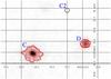 |
Fig. 5 HST WFPC2 image of HD 164492C and its surroundings obtained during a short 30.8 s exposure in the F502N filter. North is up and east to the left. The image size is |

The changes in the shape of the Stokes I and V profiles during two consecutive nights suggest that HD 164492C is either a spectroscopically variable star because of chemical spots or it is a double-lined spectroscopic binary in which the lines of the primary and the secondary appear strongly blended on both nights. The presence of the weak He ii 4686 Å line in the central strongest component indicates a spectral type B1 (for normal He content) or B1.5 (for enhanced He), implying an effective temperature of about 24 000–26 000 K (Nieva 2013). Moreover, the He lines appear in normal strength for the Teff estimated from the metal lines. Therefore a He-strong star can be excluded. To better understand the origin of the variability of this system we investigated the behaviour of a few individual elements. In Fig. 4, we display the average profiles of the best clean lines identified in the HARPS spectra. Remarkably, both the Si iii and Mg ii profiles exhibit several absorption peaks in this plot. In the same figure, the upper spectrum presents the difference between the average profiles from both nights for each element. The detected features in these difference spectra are mostly caused by the variation of the radial velocity from one night to the next, indicating that HD 164492C cannot be considered as a single star. According to the archive HST WFPC2 image of HD 164492C and its surroundings presented in Fig. 5, the source C coinciding with HD 164492C has an elongated shape, implying that we should see at least two stars in our HARPS spectra. If we assume that we observe a binary system, a reasonable interpretation of the observed line profiles might be that the main absorption peak corresponds to one star with vsini = 55 km s-1 that is superimposed on a broad-lined star with vsini of about 140 km s-1. This second fast-rotating star would contribute to the left and right wings of the profiles presented in Fig. 4. It is possible that this star also has surface chemical patches, since profiles of different elements look somewhat different. On the other hand, the relatively rapid radial velocity variation in the spectrum of the primary (~4 km s-1 per day) indicates that this star should have a close companion. Thus, we expect that the system HD 164492C is at least a triple system.
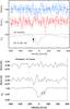 |
Fig. 6 I, V, and N profiles obtained for HD 164492C during the first night. Top panel: LSD profiles using metal lines. Bottom panel: SVD profiles using Si iii lines. The V and N profiles were expanded by factors of 25 and shifted upwards for better visibility. Additional absorption peaks are indicated by arrows. |
In the top panel of Fig. 6, we present I, V, and N LSD profiles obtained with the line mask excluding broad He i lines. In the bottom panel we show the SVD analysis where only 24 Si iii lines are included. In the SVD Stokes I Si iii line profile, the blend in the red wing of the primary appears double-peaked, while one more peak in the blue wing of the primary is best visible in the LSD Stokes I profile. The measurement of the strength of the mean longitudinal magnetic field using the first-order moment method is described by Rees & Semel (1979) and requires measuring the equivalent width of Stokes I. Because of the strong blending of the components, we are unable to estimate the strength of the detected magnetic field. Given the complex configuration and shape of the Stokes profiles, it is currently also impossible to conclude exactly which components possess a magnetic field. The detection of a significant Stokes V signature in the SVD and LSD profiles at about −100 km s-1 and +150 km s-1 from the line core of the primary suggests that more than one component might hold a magnetic field. The Stokes V profile obtained on June 3 is well centred on the position of the primary. Assuming that HD 164492C is a single star, with the SVD and LSD methods we obtain results very similar to those obtained with FORS 2: between 500 and 700 G for the first night, and 400 and 600 G for the second night.
4. Discussion
Using FORS 2 and HARPS in the framework of our ESO Large Program 191.D-0255, we detected a magnetic field in the poorly studied system HD 164492C. Although HD 164492C appears to be a multiple system, the multiplicity configuration is currently unclear and cannot be better elucidated without additional observations.
X-ray emission from HD 164492C is firmly detected using Chandra observations, but is blended with a nearby unidentified X-ray source (component C2; Rho et al. 2004). The total X-ray luminosity of these two marginally spatially resolved sources is 2 × 1032 erg s-1, with both components having similar X-ray brightness. The component C2 shows X-ray variability and is harder in X-rays than HD 164492C.
To identify and model the physical processes that are responsible for the generation of magnetic fields in massive stars, it is important to understand the formation mechanism of magnetic massive stars. Although the Trifid nebula has often been studied, its distance is not accurately known. Rho et al. (2008) reviewed literature values between 1.68 and 2.84 kpc and adopted a distance of about 1.7 kpc. Cambrésy et al. (2011) found 2.7 ± 0.5 kpc in their analysis of new near- and mid-infrared data. Torii et al. (2011) used both 1.7 and 2.7 kpc in their discussion. Even shorter distances of 816 pc and 1093 pc were estimated by Kharchenko et al. (2005; 2013) by combining proper-motion data with optical and near-infrared photometry in their cluster analysis, respectively. The spatial distribution of the components of the multiple system ADS 10991 and the photometric study by Kohoutek et al. (1999), which revealed almost the same E(B − V) values for components A–C, suggest that these components build a physical system in the nucleus of the Trifid nebula.
The age of the Trifid nebula is only a few 0.1 Myr according to Cernicharo et al. (1998), who considered the spatial extent of the H ii region. HD 164492 is a member of the cluster M20, which is probably older than 0.1 Myr and has been forming stars for longer than we discuss here. Torii et al. (2011) argued that the formation of first-generation stars in the Trifid nebula, including the main ionising O7.5 star HD 164492A, was triggered by the collision of two molecular clouds on a short time-scale of ~1 Myr. New insights into the understanding of massive star formation in the Trifid nebula can be expected from a recently established large project based on infrared and X-ray observations of 20 massive star-forming regions, among them the Trifid nebula (Feigelson et al. 2013).
The presented first detection of a magnetic massive multiple system in one of the youngest star-forming regions implies that this system may play a pivotal role in our understanding of the origin of magnetic fields in massive stars. Future spectropolarimetric monitoring of this system is urgently needed to better characterise the components, their orbital parameters, and the magnetic field topology.
Acknowledgments
We thank J. Maíz Apellániz, A. de Koter, A. Herrero, and F. Schneider for useful comments. T.M. acknowledges financial support from Belspo for contract PRODEX GAIA-DPAC.
References
- Alecian, E., Wade, G. A., Catala, C., et al. 2013, MNRAS, 429, 1001 [NASA ADS] [CrossRef] [Google Scholar]
- Bagnulo, S., Szeifert, T., Wade, G. A., et al. 2002, A&A, 389, 191 [NASA ADS] [CrossRef] [EDP Sciences] [Google Scholar]
- Bagnulo, S., Landstreet, J. D., Fossati, L., & Kochukhov, O. 2012, A&A, 538, A129 [NASA ADS] [CrossRef] [EDP Sciences] [Google Scholar]
- Cambrésy, L., Rho, J., Marshall, D. J., & Reach, W. T. 2011, A&A, 527, A141 [NASA ADS] [CrossRef] [EDP Sciences] [Google Scholar]
- Carrier, F., North, P., Udry, S., & Babel, J. 2002, A&A, 394, 1 [Google Scholar]
- Carroll, T. A., Strassmeier, K. G., Rice, J. B., & Künstler, A. 2012, A&A, 548, A95 [NASA ADS] [CrossRef] [EDP Sciences] [Google Scholar]
- Cernicharo, J., Lefloch, B., Cox, P., et al. 1998, Science, 282, 462 [NASA ADS] [CrossRef] [PubMed] [Google Scholar]
- Donati, J.-F., Semel, M., Carter, B. D., et al. 1997, MNRAS, 291, 658 [NASA ADS] [CrossRef] [MathSciNet] [Google Scholar]
- Feigelson, E. D., Townsley, L. K., Bross, P. S., et al. 2013, ApJ, 209, 26 [Google Scholar]
- Ferrario, L., Pringle, J. E, Tout, C. A, & Wickramasinghe, D. T. 2009, MNRAS, 400, L7 [Google Scholar]
- Fossati, L., Kochukhov, O., Jenkins, J. S., et al. 2013, A&A, 551, A85 [NASA ADS] [CrossRef] [EDP Sciences] [Google Scholar]
- Grunhut, J. H., Wade, G. A., & MiMeS Collaboration 2012, ASP Conf. Ser., 465, 42 [Google Scholar]
- Herbig, G. H. 1957, ApJ, 125, 654 [NASA ADS] [CrossRef] [Google Scholar]
- Hubrig, S., Kurtz, D. W., Bagnulo, S., et al. 2004a, A&A, 415, 661 [NASA ADS] [CrossRef] [EDP Sciences] [Google Scholar]
- Hubrig, S., Szeifert, T., Schöller, M., et al. 2004b, A&A, 415, 685 [NASA ADS] [CrossRef] [EDP Sciences] [Google Scholar]
- Hubrig, S., Stelzer, B., Schöller, M., et al. 2009, A&A, 502, 283 [NASA ADS] [CrossRef] [EDP Sciences] [Google Scholar]
- Hubrig, S., Schöller, M., Ilyin, I., & Lo Curto, G. 2013, Astron. Nachr., 334, 1093 [NASA ADS] [CrossRef] [Google Scholar]
- Ilyin, I. 2012, Astron. Nachr., 333, 213 [NASA ADS] [CrossRef] [Google Scholar]
- Kharchenko, N. V., Piskunov, A. E., Röser, S., et al. 2005, A&A, 438, 1163 [NASA ADS] [CrossRef] [EDP Sciences] [MathSciNet] [Google Scholar]
- Kharchenko, N. V., Piskunov, A. E., Schilbach, E., et al. 2013, A&A, 558, A53 [NASA ADS] [CrossRef] [EDP Sciences] [Google Scholar]
- Kochukhov, O., Makaganiuk, V., & Piskunov, N. 2010, A&A, 524, A5 [NASA ADS] [CrossRef] [EDP Sciences] [Google Scholar]
- Kohoutek, L., Mayer, P., & Lorenz, R. 1999, A&AS, 134, 129 [NASA ADS] [CrossRef] [EDP Sciences] [Google Scholar]
- Kupka, F. G., Ryabchikova, T. A., Piskunov, N. E., et al. 2000, Baltic Astron., 9, 590 [Google Scholar]
- Makaganiuk, V., Kochukhov, O., Piskunov, N., et al. 2011, A&A, 529, A160 [NASA ADS] [CrossRef] [EDP Sciences] [Google Scholar]
- Nieva, M. F. 2013, A&A, 550, A26 [NASA ADS] [CrossRef] [EDP Sciences] [Google Scholar]
- Piskunov, N. E., & Valenti, J. A. 2002, A&A, 385, 1095 [NASA ADS] [CrossRef] [EDP Sciences] [Google Scholar]
- Price, D. J., & Bate, M. R. 2007, MNRAS, 377, 77 [NASA ADS] [CrossRef] [Google Scholar]
- Rees, D. E., & Semel, M. D. 1979, A&A, 74, 1 [NASA ADS] [Google Scholar]
- Rho, J., Corcoran, M. F., Hamaguchi, K., & Lefloch, B. 2004, ApJ, 607, 904 [NASA ADS] [CrossRef] [Google Scholar]
- Rho, J., Lefloch, B., Reach, W. T., & Cernicharo, J. 2008, in Handbook of Star Forming Regions, Vol. II, ed. B. Reipurth, 509 [Google Scholar]
- Snik, F., Jaffers, S., Keller, C., et al. 2008, Proc. SPIE, 7014, E22 [NASA ADS] [Google Scholar]
- Sota, A., Maíz Apellániz, J., Morrell, N. I., et al. 2014, ApJS, 211, 10 [NASA ADS] [CrossRef] [Google Scholar]
- Torii, K., Enokiya, R., Sano, H., et al. 2011, ApJ, 738, 46 [NASA ADS] [CrossRef] [Google Scholar]
All Figures
|
Fig. 1 Left panel: Stokes I FORS 2 spectra of three components of the multiple system ADS 10991 (HD 164492A, HD 164492C, and HD 164492D) in the vicinity of the Hγ line. Right panel: Stokes I (top) and V / I (bottom) FORS 2 spectra of HD 164492C in the vicinity of the Hβ line. |
| In the text | |
|
Fig. 2 I, V, and N SVD profiles obtained for HD 164492C for both nights. The V and N profiles were expanded by a factor of 75 and shifted upwards for better visibility. |
| In the text | |
|
Fig. 3 I, V, and N LSD profiles (from bottom to top) obtained for HD 164492C. The V and N profiles were expanded by a factor of 75 and shifted upwards for better visibility. |
| In the text | |
|
Fig. 4 Average profiles (except for the Mg ii 4481 line) calculated using several unblended lines: five Si iii lines, ten O ii lines, and four N ii lines. For comparison, we also present the average of ten He i lines. The emission feature on the red side of the N ii profile belongs to the O iii 5006.8 Å line. For each element, the upper spectrum presents the difference between the average profiles from both nights. The apparent features in these difference spectra are mostly due to the variation of the radial velocity from one night to the next. |
| In the text | |
|
Fig. 5 HST WFPC2 image of HD 164492C and its surroundings obtained during a short 30.8 s exposure in the F502N filter. North is up and east to the left. The image size is |
| In the text | |
|
Fig. 6 I, V, and N profiles obtained for HD 164492C during the first night. Top panel: LSD profiles using metal lines. Bottom panel: SVD profiles using Si iii lines. The V and N profiles were expanded by factors of 25 and shifted upwards for better visibility. Additional absorption peaks are indicated by arrows. |
| In the text | |
Current usage metrics show cumulative count of Article Views (full-text article views including HTML views, PDF and ePub downloads, according to the available data) and Abstracts Views on Vision4Press platform.
Data correspond to usage on the plateform after 2015. The current usage metrics is available 48-96 hours after online publication and is updated daily on week days.
Initial download of the metrics may take a while.