| Issue |
A&A
Volume 564, April 2014
|
|
|---|---|---|
| Article Number | A74 | |
| Number of page(s) | 10 | |
| Section | Astrophysical processes | |
| DOI | https://doi.org/10.1051/0004-6361/201323159 | |
| Published online | 09 April 2014 | |
A two-zone approach to neutrino production in gamma-ray bursts
1
Department of PhysicsUniversity of Athens,
Panepistimiopolis,
15783
Zografou,
Greece
e-mail:
This email address is being protected from spambots. You need JavaScript enabled to view it.
2
Instituto de Investigaciones Físicas de Mar del Plata (CONICET –
UNMdP), Facultad de Ciencias Exactas y Naturales, Universidad Nacional de Mar del
Plata, Dean Funes 3350,
(7600)
Mar del Plata,
Argentina
Received:
29
November
2013
Accepted:
5
February
2014
Abstract
Context. Gamma-ray bursts (GRB) are the most powerful events in the universe. They are capable of accelerating particles to very high energies, so are strong candidates as sources of detectable astrophysical neutrinos.
Aims. We study the effects of particle acceleration and escape by implementing a two-zone model in order to assess the production of high-energy neutrinos in GRBs associated with their prompt emission.
Methods. Both primary relativistic electrons and protons are injected in a zone where an acceleration mechanism operates and dominates over the losses. The escaping particles are re-injected in a cooling zone that propagates downstream. The synchrotron photons emitted by the accelerated electrons are taken as targets for pγ interactions, which generate pions along with the pp collisions with cold protons in the flow. The distribution of these secondary pions and the decaying muons are also computed in both zones, from which the neutrino output is obtained.
Results. We find that for escape rates lower than the acceleration rate, the synchrotron emission from electrons in the acceleration zone can account for the GRB emission, and the production of neutrinos via pγ interactions in this zone becomes dominant for Eν > 105 GeV. For illustration, we compute the corresponding diffuse neutrino flux under different assumptions and show that it can reach the level of the signal recently detected by IceCube.
Key words: radiation mechanisms: non-thermal / neutrinos / gamma-ray burst: general
© ESO, 2014
1. Introduction
Gamma-ray bursts (GRBs) are intense and brief flashes of gamma rays that last from a
fraction of a second to tens of seconds, releasing energies as high as 1051−53 erg (Piran 2004; Mészáros
2006). While short bursts with durations  s are
believed to be caused by the merger of compact stars in a binary system, long bursts
(
s are
believed to be caused by the merger of compact stars in a binary system, long bursts
( s) are thought to be
triggered by the collapse of a massive star into a black hole. In the most accepted
scenario, the prompt emission corresponding to the observed burst is supposed to come from
synchrotron and/or inverse Compton emission of electrons that are accelerated in internal
shocks of ejecta with various Lorentz factors, Γ ~ 100–1000 (e.g. Rees &
Mészáros 1994; Fenimore et al. 1996; Kobayashi et al. 1997). However, this is not the only
possibility: photospheric models and acceleration by reconnection have also been proposed to
explain such emission (e.g. Mészáros & Rees
2006; Giannios 2006; Gao et al. 2011).
s) are thought to be
triggered by the collapse of a massive star into a black hole. In the most accepted
scenario, the prompt emission corresponding to the observed burst is supposed to come from
synchrotron and/or inverse Compton emission of electrons that are accelerated in internal
shocks of ejecta with various Lorentz factors, Γ ~ 100–1000 (e.g. Rees &
Mészáros 1994; Fenimore et al. 1996; Kobayashi et al. 1997). However, this is not the only
possibility: photospheric models and acceleration by reconnection have also been proposed to
explain such emission (e.g. Mészáros & Rees
2006; Giannios 2006; Gao et al. 2011).
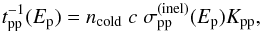
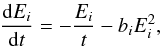
Neutrino production in GRBs is expected if, for instance, protons are co-accelerated with the electrons responsible for the prompt emission. Then, pγ and pp interactions in the baryon rich flow would lead to pion production, and thus to neutrinos (e.g. Waxman & Bahcall 1997; Guetta et al. 2004; Murase & Nagataki 2006). In more recent studies, new calculations have been developed to obtain the possible neutrino flux under different assumptions (e.g. Hümmer et al. 2012; Murase et al. 2012; Baerwald et al. 2012; He et al. 2012). It has also been proposed that in an earlier stage, while the jet is still propagating inside the collapsing star or just outside its surface, shocks may develop but without an observable photon counterpart, and only neutrinos would escape (Razzaque et al. 2004; Ando & Beacom 2005; Vieyro et al. 2013). Another well studied possibility is the generation of neutrinos during the afterglow phase (e.g. Waxman & Bahcall 2000; Dai & Lu 2001), which corresponds to a delayed low energy emission that occurs from hours to days after the prompt emission, and is commonly explained by external shocks with the interstellar medium.
In the present work, we focus on the production of prompt neutrinos, considering the effects of a generic acceleration process acting on all charged particles, including the secondary pions and muons. To do this, we adopt a simple model with two zones: an acceleration zone and a cooling one, and we assume that the particles escaping from the former are injected into the latter. We find that in the cases where the escape rate is slower than the acceleration rate, then the synchrotron emission from the electrons in the acceleration zone can yield a flux that is consistent with GRB observations. Then, the co-accelerated protons can produce significant amounts of pions by pp and pγ interactions depending on the power injected in protons. The decaying muons can undergo acceleration in the cases of higher magnetic fields, for which their acceleration rate becomes higher than their decay rate. For illustration, we compute the diffuse neutrino flux that would be expected from GRBs under some different assumptions on the Lorentz factor and on the escape rate, and we compare these results with the Waxman-Bahcall GRB flux (Waxman & Bahcall 1997) and with the data of the recent neutrino detection by IceCube (Aartsen et al. 2013).
This work is organized as follows. In Sect. 2, we describe the basic assumptions of the model, and in Sect. 3 we show the results obtained for the particle distributions: protons, electrons, pions and muons. In Sect. 4 we show illustrative results for the predicted broadband GRB photon flux, and in Sect. 5 we compute the corresponding diffuse fluxes of prompt neutrinos. The final comments are made in Sect. 6.
2. Basics of the model
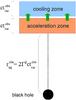 |
Fig. 1 Basic elements of the model. See text for details. |
The main components of the model are depicted in Fig. 1. The acceleration zone is the place where primary protons and electrons are
injected and accelerated. The underlying idea is that a GRB of a total duration
 s is
considered to be produced by many injection events (
s is
considered to be produced by many injection events ( ), each
responsible for a peak of duration
), each
responsible for a peak of duration  –0.01 s
in the observed lightcurve. Here, the superscripts obs correspond to a frame at the
source location, i.e., not corrected by redshift. The accelerated particles that escape are
re-injected in a second zone where they lose energy.
–0.01 s
in the observed lightcurve. Here, the superscripts obs correspond to a frame at the
source location, i.e., not corrected by redshift. The accelerated particles that escape are
re-injected in a second zone where they lose energy.
The values of the basic parameters are estimated as in previous studies (e.g. Piran 2004; Mészáros
2006). The distance from the central source to the initial position of the
acceleration zone is related to the Lorentz factor of the flow Γ and the variability time-scale as
 which,
in the case of
which,
in the case of  s,
yields 6 × 1012 cm
and 5.4 × 1013 cm for
Γ = 100 and Γ = 300, respectively.
s,
yields 6 × 1012 cm
and 5.4 × 1013 cm for
Γ = 100 and Γ = 300, respectively.
The thickness of this zone in the comoving frame is  , and its comoving volume is
 , where
 is the position of the acceleration
zone as a function of the comoving time t. For simplicity, we assume that both the
acceleration zone and cooling zone have the same volume and Lorentz factor.
is the position of the acceleration
zone as a function of the comoving time t. For simplicity, we assume that both the
acceleration zone and cooling zone have the same volume and Lorentz factor.
We suppose that the bulk kinetic energy of the flow is Ekin = 1052−53 erg, so that the
comoving number density of cold protons is given by
 (1)The magnetic energy is
assumed to be a fraction ϵB of the kinetic
energy, which implies a magnetic field (e.g. Waxman
& Bahcall 1997; Murase & Nagataki
2006; Baerwald et al. 2012):
(1)The magnetic energy is
assumed to be a fraction ϵB of the kinetic
energy, which implies a magnetic field (e.g. Waxman
& Bahcall 1997; Murase & Nagataki
2006; Baerwald et al. 2012):
 For
instance, this yields B = 4.3 × 10⁵ G for Γ = 100 and B = 1.6 × 10⁴ G
for Γ = 300 if ϵB = 0.1. In the
acceleration zone, we suppose that there is a certain mechanism that increases the energy
Ei of particles of a type
i = {e,p,π,μ} at a
rate (e.g. Begelman et al. 1990)
For
instance, this yields B = 4.3 × 10⁵ G for Γ = 100 and B = 1.6 × 10⁴ G
for Γ = 300 if ϵB = 0.1. In the
acceleration zone, we suppose that there is a certain mechanism that increases the energy
Ei of particles of a type
i = {e,p,π,μ} at a
rate (e.g. Begelman et al. 1990)  (2)where
η is an
efficiency parameter. The relation between this acceleration rate and the rate of escape
from acceleration zone the into the cooling zone will affect the energy dependence of the
particle distributions (e.g. Protheroe & Stanev
1999; Drury et al. 1999; Moraitis & Mastichiadis 2007). Here we assume
that the escape rate is some fraction of the acceleration rate,
(2)where
η is an
efficiency parameter. The relation between this acceleration rate and the rate of escape
from acceleration zone the into the cooling zone will affect the energy dependence of the
particle distributions (e.g. Protheroe & Stanev
1999; Drury et al. 1999; Moraitis & Mastichiadis 2007). Here we assume
that the escape rate is some fraction of the acceleration rate,
 (3)A
reference case is the one where ξesc = 1, which yields distributions
proportional to E-2 in the cooling zone (Kirk et al. 1998). Still, in the present work we explore
situations in which ξesc < 1, since we
are not specifying the nature of the acceleration mechanism and are exploring different
cases in the context of GRBs1.
(3)A
reference case is the one where ξesc = 1, which yields distributions
proportional to E-2 in the cooling zone (Kirk et al. 1998). Still, in the present work we explore
situations in which ξesc < 1, since we
are not specifying the nature of the acceleration mechanism and are exploring different
cases in the context of GRBs1.
We next comment on the cooling processes, and we leave the question of the particle distributions and the method of calculation for Sect. 3.
 |
Fig. 2 Acceleration and cooling rates for electrons and protons for a bulk Lorentz factor
Γ = 100 and
300 in the top
and bottom panels, respectively. The labels SSC-a(c) and
pγ-a(c)
indicate the respective processes for the acceleration (cooling) zone. The escape rate
shown is |

2.1. Cooling processes
The synchrotron energy loss rate, in the CGS system of units, is  (4)We consider an adiabatic
cooling with a rate similar to the inverse of the dynamical timescale (e.g. Murase & Nagataki 2006),
(4)We consider an adiabatic
cooling with a rate similar to the inverse of the dynamical timescale (e.g. Murase & Nagataki 2006),
 (5)where
t is the
comoving time.
(5)where
t is the
comoving time.
To compute the inverse Compton cooling rate, a soft photon field is necessary as a target
for the electrons. We assume that these soft photons are mainly due to the synchrotron
radiation of the same electron population, which have a differential density (in units of
energy-1length-3)
 (6)where the synchrotron
emissivity, in units of (energy-1length-3sr-1time-1),
is
(6)where the synchrotron
emissivity, in units of (energy-1length-3sr-1time-1),
is  (7)Here,
Ne is the electron distribution in units
of (energy-1length-3), K5/3(ζ)
is the modified Bessel function of order 5/3, and the critical energy, close to the peak
of the synchrotron spectrum, is (e.g. Blumenthal &
Gould 1970)
(7)Here,
Ne is the electron distribution in units
of (energy-1length-3), K5/3(ζ)
is the modified Bessel function of order 5/3, and the critical energy, close to the peak
of the synchrotron spectrum, is (e.g. Blumenthal &
Gould 1970)  in
the comoving frame.
in
the comoving frame.
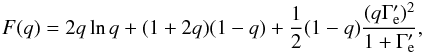
The synchrotron self-Compton cooling rate is then approximated by (e.g. Jones 1968) ![Mathematical equation: \begin{eqnarray} {t}^{-1}_{\rm SSC}(E_{\rm e},t)&= &\frac{3 m_{\rm e}^2 c^5 \sigma_{\rm T}}{4 {E}^3}\int_{{E}_{\rm ph}^{\rm(min)}}^{E_{\rm e}}{\rm d}E_{\rm ph } \frac{n_{\gamma}(E_{\rm ph},t)}{{E}_{\rm ph}}\nonumber \\ &&\times \int_{{E}_{\rm ph}}^{\frac{\Gamma_{\rm e}}{\Gamma_{\rm e}+1}E_{\rm e}} {\rm d}E_\gamma F(q)\left[E_\gamma-E_{ \rm ph}\right], \label{tIC} \end{eqnarray}](/articles/aa/full_html/2014/04/aa23159-13/aa23159-13-eq49.png) (8)where
(8)where
 is
the lowest energy of the available background of synchrotron photons, and
is
the lowest energy of the available background of synchrotron photons, and
 (9)with
 and
and
![Mathematical equation: \hbox{$q={E_\gamma}\left[{\Gamma_{\rm e}E_{\rm ph}(1-{E_\gamma/}{E_{\rm ph}})}\right]^{-1}.$}](/articles/aa/full_html/2014/04/aa23159-13/aa23159-13-eq53.png) As for
protons, the pγ cooling rate is
As for
protons, the pγ cooling rate is  (10)where,
 MeV, and we use the
expressions for the cross section
MeV, and we use the
expressions for the cross section  and
the inelasticity
and
the inelasticity  given
in Atoyan & Dermer (2003). The e+e− pair production by pγ collisions (Bethe-Heitler
process) was also included as in the
given
in Atoyan & Dermer (2003). The e+e− pair production by pγ collisions (Bethe-Heitler
process) was also included as in the  following Begelman et al. (1990).
Parameters of the model.
 |
Fig. 3 Rates of acceleration, escape, decay, and cooling for pions and muons. The top panels correspond to Γ = 100 and the bottom ones to Γ = 300. |
The energy loss rate due to inelastic pp collisions is
 (11)where
the inelasticity coefficient is Kpp ≈ 1/2 and the
corresponding cross section can be approximated as in Kelner et al. (2006).
(11)where
the inelasticity coefficient is Kpp ≈ 1/2 and the
corresponding cross section can be approximated as in Kelner et al. (2006).
For the parameter values of Table 1, we show in Fig. 2 the acceleration and cooling rates for electrons and protons, separating the cases of Γ = 100 and Γ = 300 in the upper and lower panels, respectively. Here we note that the rates are much lower for Γ = 300 than for Γ = 100, which will require more energy to be injected in the former case in order to have similar radiative outputs, as we will see below. The escape rate is also shown, which in this case is a fraction ξesc = 0.1 of the acceleration rate as mentioned above. The acceleration and cooling rates for pions and muons are shown in Fig. 3, where the corresponding decay rates are also included.
3. Particle distributions
To obtain the distribution of each particle type i = {e,p,π,μ} in
each zone, we solve the general kinetic equation ![Mathematical equation: \begin{equation} \frac{\partial N_{i}}{\partial t} +\frac{\partial\left[\dot{E}_{i} N_{i,}\right]}{\partial E_i} + \frac{N_{i}}{t_{\rm esc}}= Q_i(E_i,t) \label{kineticeq}, \end{equation}](/articles/aa/full_html/2014/04/aa23159-13/aa23159-13-eq91.png) (12)where Qi is the injection term in
units of (energy-1length-3time-1), and the
energy change is
(12)where Qi is the injection term in
units of (energy-1length-3time-1), and the
energy change is  .
The escape term is only present for particles in the acceleration zone, and in the case of
pions and muons, the term of decay
.
The escape term is only present for particles in the acceleration zone, and in the case of
pions and muons, the term of decay  must be
also added in the left-hand side.
must be
also added in the left-hand side.
For the primary electrons and protons (i = { e,p }) in the acceleration
zone, where acceleration is assumed to operate during the time of the injection event
 in the
comoving frame, we use a mono-energetic injection
in the
comoving frame, we use a mono-energetic injection
 (13)Here
H is the
Heaviside step function, γinj the Lorentz factor of the injected
particles, and Ki a normalization
constant
(13)Here
H is the
Heaviside step function, γinj the Lorentz factor of the injected
particles, and Ki a normalization
constant  (14)This one is fixed by the
corresponding power injected in the comoving frame during the time tvar:
(14)This one is fixed by the
corresponding power injected in the comoving frame during the time tvar:
 (15)For instance, with the
parameter values of Table 1 we obtain LGRB = { 5 × 1047erg s-1; 5.5 × 1046 erg s-1 }
for Γ = 100 and Γ = 300, respectively. The corresponding
values of qi are those that yield
the values of Li appearing in Table
1: qe ~ 8 × 10⁻⁴ and
qp ~ 6 × 10⁻⁵ for
Γ = 100, and qe ~ 2 × 10⁻⁴ and qp ~ 0.1 for
Γ = 300.
(15)For instance, with the
parameter values of Table 1 we obtain LGRB = { 5 × 1047erg s-1; 5.5 × 1046 erg s-1 }
for Γ = 100 and Γ = 300, respectively. The corresponding
values of qi are those that yield
the values of Li appearing in Table
1: qe ~ 8 × 10⁻⁴ and
qp ~ 6 × 10⁻⁵ for
Γ = 100, and qe ~ 2 × 10⁻⁴ and qp ~ 0.1 for
Γ = 300.
The energy change in the acceleration zone includes both acceleration and losses,
![Mathematical equation: \begin{equation} \dot{E}_i(E_i)= E_i\times \left[t^{-1}_{\rm acc}(E_i) -t^{-1}_{i,\rm{loss}}(E_i) \right], \end{equation}](/articles/aa/full_html/2014/04/aa23159-13/aa23159-13-eq112.png) (16)and the solution can
be found using the method of the characteristics, through
(16)and the solution can
be found using the method of the characteristics, through ![Mathematical equation: \begin{equation} N_i(E_i,t)= \int_{t_0}^t {\rm d}t'Q_i(E',t')\exp\left[-\int_{t'}^{t} {\rm d}t''\left(\frac{\partial \dot{E}_i}{\partial E_i}- t^{-1}_{\rm esc} \right) \right], \label{Solformal} \end{equation}](/articles/aa/full_html/2014/04/aa23159-13/aa23159-13-eq113.png) (17)which has units of
(energy-1length-3). In the case of pions and muons,
the effect of decay is included by replacing
(17)which has units of
(energy-1length-3). In the case of pions and muons,
the effect of decay is included by replacing  .
.
The process of calculation of the different particle distributions is as follows. We start
by computing the electron distribution in the acceleration zone,
 , taking acceleration and
synchrotron cooling into account. As can be seen in Fig. 2, adiabatic cooling for electrons is not important, and neither is the
synchrotron self-Compton cooling at high energies for typical GRB parameters (see Table
1). We then compute the proton distribution
, taking acceleration and
synchrotron cooling into account. As can be seen in Fig. 2, adiabatic cooling for electrons is not important, and neither is the
synchrotron self-Compton cooling at high energies for typical GRB parameters (see Table
1). We then compute the proton distribution
 considering acceleration, adiabatic
cooling, synchrotron cooling, pp interactions, and pγ interactions with the
synchrotron photons of electrons as targets. In the third place, we compute the injection of
pions
considering acceleration, adiabatic
cooling, synchrotron cooling, pp interactions, and pγ interactions with the
synchrotron photons of electrons as targets. In the third place, we compute the injection of
pions  by both pp and pγ collisions and use it in
the right-hand side of Eq. (12) to obtain
the distributions of pions in the acceleration zone,
by both pp and pγ collisions and use it in
the right-hand side of Eq. (12) to obtain
the distributions of pions in the acceleration zone,  . After this, we compute the
injection of muons
. After this, we compute the
injection of muons  and obtain
 .
.
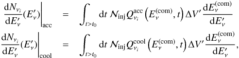
Particles escaping from the acceleration zone are re-injected in the cooling zone, with an
injection  . We solve Eq. (12) without any acceleration to obtain each
 following the same order as for the
acceleration zone.
following the same order as for the
acceleration zone.
The most important cooling mechanisms for all particle types are synchrotron and adiabatic
cooling, so that we can write a characteristic equation:
 (18)where
the first term is the adiabatic energy loss and the second term is the synchrotron energy
loss assuming for simplicity a constant magnetic field, with
(18)where
the first term is the adiabatic energy loss and the second term is the synchrotron energy
loss assuming for simplicity a constant magnetic field, with
 The
solution can be found as in Kardashev (1962), using the characteristic curve that gives the
energy E′ > E
for early times t′ < t,
The
solution can be found as in Kardashev (1962), using the characteristic curve that gives the
energy E′ > E
for early times t′ < t,
 (19)and
substituting in Eq. (17). In Fig. 4, we show the distributions of electrons and protons
evaluated at different times in the acceleration and in the cooling zone. The initial times
used are
(19)and
substituting in Eq. (17). In Fig. 4, we show the distributions of electrons and protons
evaluated at different times in the acceleration and in the cooling zone. The initial times
used are  for
Γ = { 100,300 }, which also correspond to the
injection periods in each case. Pile-ups occur at the maximum energy where the acceleration
rate equals the cooling one. Although a divergence appears at exactly this energy, the
injected particles never reach it because there is a time limitation given by the duration
of injection. In the case of electrons, the synchrotron cooling is so fast that once the
injection is switched off, there are no more high energy electrons in both zones, while the
protons take a much longer time to lose their energy. We note that the distributions in the
cooling zone are steeper than those in the acceleration zone because of the ∝
for
Γ = { 100,300 }, which also correspond to the
injection periods in each case. Pile-ups occur at the maximum energy where the acceleration
rate equals the cooling one. Although a divergence appears at exactly this energy, the
injected particles never reach it because there is a time limitation given by the duration
of injection. In the case of electrons, the synchrotron cooling is so fast that once the
injection is switched off, there are no more high energy electrons in both zones, while the
protons take a much longer time to lose their energy. We note that the distributions in the
cooling zone are steeper than those in the acceleration zone because of the ∝ dependence assumed for the escape rate, and this gives a high density distribution for low
energies in the cooling zone, as compared to the acceleration zone.
dependence assumed for the escape rate, and this gives a high density distribution for low
energies in the cooling zone, as compared to the acceleration zone.
As for the energy involved, in addition to the power injected in mono-energetic electrons
and protons (Li, see Table 1), particles undergo acceleration up to a maximum
energy, experience losses, and a fraction of them can escape to the cooling zone. As a
result, the total energy that is given to the particles can be computed as
 , with
 In
the cases studied, we obtainthe values shown in Table 1 for Γ = 100 and
Γ = 300, which are found to
produce a similar level of radiation and neutrinos as we see below. The main difference is
that protons in the case of Γ = 300, a much higher energy has to be given to the proton population
because their cooling efficiency is much lower than in the case with Γ = 100.
In
the cases studied, we obtainthe values shown in Table 1 for Γ = 100 and
Γ = 300, which are found to
produce a similar level of radiation and neutrinos as we see below. The main difference is
that protons in the case of Γ = 300, a much higher energy has to be given to the proton population
because their cooling efficiency is much lower than in the case with Γ = 100.
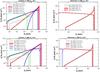 |
Fig. 4 Distributions of electrons and protons multiplied by the squared energy and evaluated at different times corresponding to the acceleration zone (solid lines) and to the cooling zone (dashed lines), for Γ = 100 (top panels) and Γ = 300 (bottom panels). |
We now describe how we compute the injection of the secondary particles.
3.1. Pions
Proton interactions with protons and low energy photons produce pions. The pion injection
due to pp collisions is is calculated as  (23)where
the distribution of pions produced per pp collision is (Kelner et al. 2006)
(23)where
the distribution of pions produced per pp collision is (Kelner et al. 2006)  (24)with
x = Eπ/E′,
Bπ = a′ + 0.25,
a′ = 3.67 + 0.83L + 0.075L2,
(24)with
x = Eπ/E′,
Bπ = a′ + 0.25,
a′ = 3.67 + 0.83L + 0.075L2,
 ,
and
,
and  .
.
Similarly, the injection of charged pions produced by pγ interactions is
 (25)Here,
 is the
pγ
collision frequency defined as (Atoyan & Dermer
2003)
is the
pγ
collision frequency defined as (Atoyan & Dermer
2003) 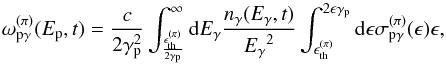 (26)and the mean
number of π+’s or π−’s is
approximately
(26)and the mean
number of π+’s or π−’s is
approximately  (27)This
number depends on the probabilities of single pion and multi-pion production
p1 and p2 = 1 − p1.
Given that the mean inelasticity function is
(27)This
number depends on the probabilities of single pion and multi-pion production
p1 and p2 = 1 − p1.
Given that the mean inelasticity function is  ,
we have
,
we have  (28)where
K1 = 0.2 and K2 = 0.6.
(28)where
K1 = 0.2 and K2 = 0.6.
 |
Fig. 5 Distributions of pions and muons multiplied by the squared energy and evaluated at different times corresponding to the acceleration zone (solid lines) and to the cooling zone (dashed lines), for Γ = 100 (top panels) and Γ = 300 (bottom panels). |
3.2. Muons
The injection of muons is treated following Lipari et al. (2007), considering left-handed
and right-handed muons separately with their decay spectra:
 where
x = Eμ/Eπ
and rπ = (mμ/mπ)2.
where
x = Eμ/Eπ
and rπ = (mμ/mπ)2.
Assuming CP invariance implies 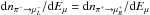 , and since the total
distribution obtained for all charged pions is Nπ = Nπ+ + Nπ−,
the injection of left-handed muons is
, and since the total
distribution obtained for all charged pions is Nπ = Nπ+ + Nπ−,
the injection of left-handed muons is  (31)Similarly, the
injection of right-handed muons is
(31)Similarly, the
injection of right-handed muons is  (32)In Fig. 5, we show the obtained distributions of pions and muons
in both zones at different times. The bumps in the distributions at energies around
~104 GeV is due
to the contribution of pγ interactions that becomes greater than that of pp.
In the particular case of muons for Γ = 100, the peak is more pronounced because muons are undergoing
acceleration, and the maximum energy where acceleration equals losses is also around
~104 GeV. In the
cooling zone, the pion injection is dominated by the produced by pγ and pp interactions in
this zone, since the decay rate is much greater than the escape rate for the cases studied
here, so pions generated in the acceleration zone will decay there, as can be seen in Fig.
3. For muons, the decay is slower, so for
ξesc > 0.1, the
escape rate approaches the decay rate, and there is a non-negligible injection of escaping
muons into the cooling zone, which is added up to the contribution coming from pions
created in the cooling zone itself.
(32)In Fig. 5, we show the obtained distributions of pions and muons
in both zones at different times. The bumps in the distributions at energies around
~104 GeV is due
to the contribution of pγ interactions that becomes greater than that of pp.
In the particular case of muons for Γ = 100, the peak is more pronounced because muons are undergoing
acceleration, and the maximum energy where acceleration equals losses is also around
~104 GeV. In the
cooling zone, the pion injection is dominated by the produced by pγ and pp interactions in
this zone, since the decay rate is much greater than the escape rate for the cases studied
here, so pions generated in the acceleration zone will decay there, as can be seen in Fig.
3. For muons, the decay is slower, so for
ξesc > 0.1, the
escape rate approaches the decay rate, and there is a non-negligible injection of escaping
muons into the cooling zone, which is added up to the contribution coming from pions
created in the cooling zone itself.
4. Electromagnetic emission
 |
Fig. 6 SED of photons obtained for a GRB with Γ = 100 (top panels) and with Γ = 300 (bottom panels) originated in both the acceleration zone (solid lines with circles) and in the cooling zone at different times (solid lines). A typical GRB photon field is shown for comparison in a thick dashed grey line. The dominant processes are included: electron synchrotron (blue), inverse Compton (black), muon synchrotron (cyan), secondary e + e − synchrotron (green), pγ (purple), and pp (orange). The different values adopted for ξesc are indicated. |
Here we present results for the broadband photon emission produced by the different
particle populations in both zones of the present model. We chose two cases in which the
escape rate is slower than the acceleration rate since this can give rise to significant
synchrotron emission of electrons in the acceleration zone. The peak of this emission is
related to the maximum energy of the electrons, which depends on the magnetic field and on
the efficiency of the acceleration η. We find that this peak can fall within the correct
energy range and intensity as turns out when we compare it with a usually adopted spectrum
for GRBs, the following broken power law (e.g. Murase
& Nagataki 2006; Lipari et al. 2007;
Baerwald et al. 2012):
 (33)Here,
the constant Cγ is fixed by
specifying the energy density of these population of photons, which we take to be equal to
the magnetic energy density, as assumed in the works mentioned.
(33)Here,
the constant Cγ is fixed by
specifying the energy density of these population of photons, which we take to be equal to
the magnetic energy density, as assumed in the works mentioned.
In Fig. 6 we show the spectral energy density (SED) of photons corresponding to this broken power law profile, and we include all the relevant contributions within our model arising from the processes in both zones evaluated at the time of maximum emission, t = t0 + tvar. The synchrotron emission from electrons has been corrected for synchrotron self absorption, which is important for the contribution of the cooling zone. In each panel, we show the value of the obtained fraction energy in protons divided by the total energy in electrons, ΔEp/ΔEe. The very high-energy contributions shown (pγ, pp, and e+e− synchrotron) are not corrected for γγ absorption in order to appreciate their intrinsic intensities. Also, since the redshift chosen for the example GRB is z = 1.8, γγ annihilations of gamma-rays on the extragalactic background light (EBL) would cause complete absorption for Eγ ≳ 100 GeV (e.g. Inoue et al. 2012).
Although we are not interested here in making predictions for the VHE photons and their detectability, for completeness we computed the synchrotron emission of a first generation of secondary e+e− created by the decay of muons to verify that it does not overcome the synchrotron emission of the primary electrons, which is taken as the primary target for pγ interactions. We obtained the corresponding distribution Nμ → e± as a solution of the kinetic equation with an injection taken to be equal to that of νe, using the expression listed below after Lipari et al. (2007). Formally, a cascade will develop after internal γγ absorption, creating more pairs that will again radiate synchrotron photons and that can also get absorbed (e.g. Asano et al. 2010). While a complete treatment of such a cascade would give the final shape and intensity of the spectrum, we have checked that the synchrotron emission of the first generation of e+e− pairs resulting from internal γγ absorption (Aharonian et al. 1983) is not greater than the emission from electrons and positrons from muon decays, as can be seen in Fig. 6. Hence, assuming that after the full cascade the high energy part is reprocessed to lower energies, the expected intensity is not so high, and then the low energy photon field remains dominated by the synchrotron of primary electrons in each of the zones. This ensures that the neutrino output that we shall obtain from pγ interactions is a good approximation in the cases studied.
We can point out a difference in the SED between the cases with different Lorentz factor. In the case of Γ = 100, muons undergo acceleration because the magnetic field is higher, so the acceleration rate is greater than the decay rate. As a consequence, there is high synchrotron emission of these muons, unlike the case with Γ = 300, for which the magnetic field is lower and there is no significant muon acceleration. Other important difference between these two cases is clear through the values of the fraction ΔEp/ΔEe. As mentioned above, much more energy has to be present in protons in the case of Γ = 300 in order to reach the same level of pγ and pp emissions as for Γ = 100. This is because in the latter case, the corresponding cooling rates are much lower than the adiabatic cooling rate, making the proton emission processes less efficient.
5. Neutrino emission
Once we have the distributions of pions and muons, we can obtain the corresponding neutrino
emissivities arising from their decay. The contribution to muon neutrinos and antineutrinos
from the direct decay of pions is given by (e.g. Lipari
et al. 2007), 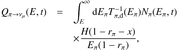 (34)with
x = E/Eπ
and the decay timescale is Tπ,d = 2.6 × 10⁻⁸ s.
The contribution from muon decays (
(34)with
x = E/Eπ
and the decay timescale is Tπ,d = 2.6 × 10⁻⁸ s.
The contribution from muon decays ( ,
,
 )
to muon neutrinos and antineutrinos is
)
to muon neutrinos and antineutrinos is
![Mathematical equation: \begin{eqnarray} Q_{\mu\rightarrow\nu_\mu}(E,t)&=& \sum_{i=1}^4\int_{E}^{\infty}\frac{{\rm d}E_\mu}{E_\mu} T^{-1}_{\mu,\rm d}(E_\mu)N_{\mu_i}(E_\mu,t) \nonumber\\&& \times \left[\frac{5}{3}- 3x^2+\frac{4}{3}x^3 +\left(3x^2-\frac{1}{3}-\frac{8x^3}{3}\right)h_{i} \right], \end{eqnarray}](/articles/aa/full_html/2014/04/aa23159-13/aa23159-13-eq178.png) (35)where
x = E/Eμ,
(35)where
x = E/Eμ,
 ,
Tμ,d = 2.2 × 10⁻⁶ s,
and
,
Tμ,d = 2.2 × 10⁻⁶ s,
and  ,
and the helicity of the muons is h = 1 for right-handed and h = −1 for left-handed
muons. Similarly, the emissivity of electron neutrinos and antineutrinos from the decay of
muons is given by
,
and the helicity of the muons is h = 1 for right-handed and h = −1 for left-handed
muons. Similarly, the emissivity of electron neutrinos and antineutrinos from the decay of
muons is given by ![Mathematical equation: \begin{eqnarray} Q_{\mu\rightarrow\nu_{\rm e}}(E,t)&=& \sum_{i=1}^4\int_{E}^{\infty}\frac{{\rm d}E_\mu}{E_\mu} T^{-1}_{\mu,\rm d}(E_\mu)N_{\mu_i}(E_\mu,t) \nonumber\\ &&\times \left[2- 6x^2+4x^3 +\left(2- 12x+ 18x^2-8x^3\right)h_{i}\right]. \end{eqnarray}](/articles/aa/full_html/2014/04/aa23159-13/aa23159-13-eq185.png) (36)The
fluence obtained for a typical GRB is the sum of the contribution from both zones:
(36)The
fluence obtained for a typical GRB is the sum of the contribution from both zones:
 where
where
 is the
total
is the
total  or
or  neutrino emissivity for the acceleration and cooling zones, in units (energy-1time-1length-3);
Eν is the neutrino energy
for z = 0, the
local neutrino energy is
neutrino emissivity for the acceleration and cooling zones, in units (energy-1time-1length-3);
Eν is the neutrino energy
for z = 0, the
local neutrino energy is  , and the comoving one in the
ejected flow is
, and the comoving one in the
ejected flow is  .
.
 |
Fig. 7 Diffuse flux of muon neutrinos predicted for GRBs, associated to their prompt emission in the case of Γ = 100 (top panels) and Γ = 300 (bottom panels) for ξesc = 0.25 and ξesc = 0.1 in the left and right panels, respectively. The contribution from the acceleration zone is marked in red and the one from the cooling zone in blue. The reference Waxman-Bahcall flux is also shown for comparison. |
Considering the GRB redshift evolution rate (e.g. Murase
& Nagataki 2006) 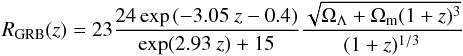 (37)in
units of (Gpc-3yr-1), the diffuse muon neutrino flux from
GRBs can then be integrated in redshift:
(37)in
units of (Gpc-3yr-1), the diffuse muon neutrino flux from
GRBs can then be integrated in redshift: ![Mathematical equation: \begin{eqnarray} \Phi_{\nu_\mu}(E_\nu)&=& \frac{c}{4\pi H_0}\int_0^{z_{\rm max}}\frac{{\rm d}z \ R_{\rm GRB(z)}}{\sqrt{\Omega_\Lambda+ \Omega_{\rm m}(1+z)^{3}}} \nonumber \\ \label{dflunudiff} &&\times \left(\frac{{\rm d}N_{\nu_\mu}\left[E_\nu(1+z)\right]}{{\rm d}E'_\nu} {P_{\nu_{\mu}\rightarrow \nu_{\mu}}}+ \frac{{\rm d}N_{\nu_{\rm e}}\left[E_\nu(1+z)\right]}{{\rm d}E'_\nu} {P_{\nu_{\rm e}\rightarrow \nu_{\mu}}}\right), \end{eqnarray}](/articles/aa/full_html/2014/04/aa23159-13/aa23159-13-eq199.png) (38)where
ΩΛ = 0.7,
Ωm = 0.3, and
H0 = 70 km s-1 Mpc-1.
The effect of neutrino flavour oscillation is taken into account in Eq. (38) through the probability that the generated
νμ and
(38)where
ΩΛ = 0.7,
Ωm = 0.3, and
H0 = 70 km s-1 Mpc-1.
The effect of neutrino flavour oscillation is taken into account in Eq. (38) through the probability that the generated
νμ and
 remain of the same flavour, Pνμ → νμ,
and also through the probability that electron neutrinos or antineutrinos and oscillate into
muon neutrinos or antineutrinos, Pνe → νμ.
These probabilities depend on the unitary mixing matrix Uαj, which is determined by
the three mixing angles θ12 ≃ 34°, θ13 ≃ 9°, and θ23 ≃ 45°, and a CP violating
phase which we take to be zero. The values of these angles are derived from global fits to
experimental data of solar, atmospheric, and accelerator neutrinos (e.g. Gonzalez-García et al. 2012), which yield the values for
the probabilities Pνμ→νμ = 0.369
and Pνe→νμ ≃ 0.255.
remain of the same flavour, Pνμ → νμ,
and also through the probability that electron neutrinos or antineutrinos and oscillate into
muon neutrinos or antineutrinos, Pνe → νμ.
These probabilities depend on the unitary mixing matrix Uαj, which is determined by
the three mixing angles θ12 ≃ 34°, θ13 ≃ 9°, and θ23 ≃ 45°, and a CP violating
phase which we take to be zero. The values of these angles are derived from global fits to
experimental data of solar, atmospheric, and accelerator neutrinos (e.g. Gonzalez-García et al. 2012), which yield the values for
the probabilities Pνμ→νμ = 0.369
and Pνe→νμ ≃ 0.255.
In Fig. 7, we show the different outputs for the background of muon neutrinos using Γ = 100 and Γ = 300, and with an escape-to-acceleration rate ratio of ξesc = 0.25 and ξesc = 0.1. For illustration, the parameters regulating the injected power (Le and Lp) and the efficiency of acceleration (η) have been chosen in order to obtain both a correct electron synchrotron emission (as compared to the typical broken power-law SED) and, at the same time, a neutrino flux at the level of the recent detection by IceCube (Klein 2013; Liu et al. 2013). The effect of increasing η would yield neutrinos that are more energetic than ~106 GeV and would also bring the electron synchrotron peak to higher energies, which would still be consistent with photon observations. If in light of new neutrino data (Aartsen et al. 2013) or clues disfavouring the association of the neutrino events with GRBs, it will be possible to exclude too high values of the injected power Lp in the context of the present model.
6. Discussion
We have implemented a simple two-zone model in order to study the generation of high energy neutrinos associated with the prompt GRB emission. Using standard values for the magnetic field and size of the emission region, our model can account for the possible effect of the acceleration of secondary particles. In particular, we found that muons can efficiently gain energy if the magnetic field is strong enough, but still within attainable values in the context of GRBs. We note that these effects cannot be described with previous one-zone models that deal with neutrino emission in a magnetized environment (e.g. Reynoso & Romero 2009; Baerwald et al. 2012), in which the acceleration rate is only used to fix the maximum energy of the primary electrons and protons.
As recognized in previous works (e.g. Kirk et al. 1998), particle acceleration can be accounted for using two zones and assuming that particles can escape from the acceleration zone to the cooling zone. We have not considered that particles in the cooling zone can further escape to a third zone in order not to miss their photon and neutrino output. The present model also differs from previous two-zone models in that the size of both zones are equal, and with a value derived from variability considerations. Including adiabatic losses for protons provides a mechanism for their faster cooling, on a timescale similar to the dynamical time, e.g. the one associated with the duration of the shell collision event in the internal shock scenario. A variation of the present model could be implemented by including a convective term in the kinetic equation for the cooling zone (e.g. Reynoso et al. 2011). This would prevent us from having to impose a fixed size for the cooling zone, since particles of different species and energies would reach different distances as they cool.
In the context studied here, we have found that if the escape rate is less than the acceleration rate (ξesc < 1), then the synchrotron emission from electrons in the acceleration zone dominates and can be the responsible for the usual GRB emission. Otherwise, for faster escape rates, the synchrotron emission from electrons in the cooling zone would dominate but with too wide a spectrum, which would greatly exceed the typical GRB emission at lower energies. As can be seen in Fig. 6, for lower values of ξesc, we obtain less significant electron synchrotron components from the cooling zone, and the bump corresponding to the acceleration zone falls within the correct energy range, as compared with the broken power-law benchmark. By varying the acceleration efficiency of the different injection events (such as shell collisions in the internal shock model), different maximum energies for the electrons could be achieved, and their synchrotron emission would cover a window in the gamma-ray spectrum to be consistent with a full burst. In the cases with a low escape rate, we found that a neutrino component arising from the acceleration zone mainly by pγ interactions becomes dominant at the highest neutrino energies, which in the examples shown reached ~106 GeV and can account for the recent IceCube data.
Some tasks could help make a more accurate calculation of the diffuse neutrino background in the context of the present type of models for GRBs: try to reproduce the observed gamma-ray spectrum of particular bursts by adjusting the number of acceleration events (peaks in the lightcurve) and the acceleration efficiency, and also to consider the probability of occurrence of bursts with different Lorentz factors. We leave these points for future work, along with the possible application of the model to other type of astrophysical sources.
We note, for example, that even cases with ξesc ≪ 1 have been proposed in photospheric dissipative models (e.g. Bosch-Ramon 2012; Drury 2012; Gao et al. 2011).
Acknowledgments
I am especially thankful to Prof. A. Mastichiadis for many discussions, suggestions, and help, and I thank Stavros Dimitriakoudis and Maria Petropoulou for fruitful discussions on GRB physics. I also thank the referee P. Mészáros for a helpful review. Finally, I thank CONICET (Argentina) and Agencia (Argentina) through grant PICT 2012-2621 for their financial support, and I thank the University of Athens for their hospitality.
References
- Aartsen, M. G., et al. (IceCube Collaboration) 2013, Science, 342, 6161 [Google Scholar]
- Aharonian, F. A., Atoyan, A. M., & Nagapetian, A. M. 1983, Astrofizika, 19, 323 [NASA ADS] [Google Scholar]
- Ando, S., & Beacom, J. F. 2005, Phys. Rev. Lett., 95, 061103 [NASA ADS] [CrossRef] [PubMed] [Google Scholar]
- Asano, K., Inoue, S., & Meszaros, P. 2010, ApJ, 725, L121 [NASA ADS] [CrossRef] [Google Scholar]
- Atoyan, A. M., & Dermer, C. D. 2003, ApJ, 586, 79 [NASA ADS] [CrossRef] [Google Scholar]
- Baerwald, P., Hümmer, S., & Winter, W. 2012, Astropart. Phys., 35, 508 [NASA ADS] [CrossRef] [Google Scholar]
- Begelman, M. C., Rudak, B., & Sikora, M. 1990, ApJ, 362, 38 [NASA ADS] [CrossRef] [Google Scholar]
- Blumenthal, G. R., & Gould, R. J. 1970, Rev. Mod. Phys., 42, 237 [NASA ADS] [CrossRef] [Google Scholar]
- Bosch-Ramon, V. 2012, A&A, 542, A125 [NASA ADS] [CrossRef] [EDP Sciences] [Google Scholar]
- Dai, Z. G., & Lu, T. 2001, ApJ, 551, 249 [NASA ADS] [CrossRef] [Google Scholar]
- Drury, L. 2012, MNRAS, 422, 2474 [NASA ADS] [CrossRef] [Google Scholar]
- Drury, L., Duffy, P., Eichler, D., & Mastichiadis, A. 1999, A&A, 347, 370 [NASA ADS] [Google Scholar]
- Fenimore, F. E., Madras, C. D., & Nayakshin, S. 1996, ApJ, 473, 998 [NASA ADS] [CrossRef] [Google Scholar]
- Fletcher, R. S., Gaisser, T. K., Lipari, P., & Stanev, T. 1994, Phys. Rev. D, 50, 5710 [NASA ADS] [CrossRef] [Google Scholar]
- Gao, S., Asano, K., & Meszaros, P. 2011, JCAP, 1211, 058 [NASA ADS] [CrossRef] [Google Scholar]
- Giannios, D. 2006, A&A, 457, 763 [NASA ADS] [CrossRef] [EDP Sciences] [Google Scholar]
- Gonzalez-García, M. C, Maltoni, M., Salvado, J., & Schwetz, T. 2012, J. High Energy Phys., 1212, 123 [NASA ADS] [CrossRef] [Google Scholar]
- Guetta, D., Hooper, D., Alvarez-Muiz, J., Halzen, F., & Reuveni, E. 2004, Astropart. Phys., 20, 429 [NASA ADS] [CrossRef] [Google Scholar]
- He, H.-N., Liu, R.-Y., Wang, X.-Y., et al. 2012, ApJ, 752, 29 [NASA ADS] [CrossRef] [Google Scholar]
- Hümmer, S., Baerwald, P., & Winter, W. 2012, Phys. Rev. Lett., 108, 1101 [Google Scholar]
- Inoue, Y., Inoue, S., Kobayashi, M. A. R., et al. 2013, ApJ, 768, 197 [NASA ADS] [CrossRef] [Google Scholar]
- Jones, F. C. 1968, Phys. Rev., 167, 1159 [NASA ADS] [CrossRef] [Google Scholar]
- Kardashev, N. S. 1962, SvA, 6, 317 [Google Scholar]
- Kelner, S. R., Aharonian, F. A., & Bugayov, V. V. 2006, Phys. Rev. D, 74, 4018 [Google Scholar]
- Kirk, J. G., Rieger, F. M., & Mastichiadis, A. 1998, A&A, 333, 452 [NASA ADS] [Google Scholar]
- Klein, S. 2013, Highlight talk, Proc. ICRC 2013 [Google Scholar]
- Kobayashi, S., Piran, T., & Sari, R. 1997, ApJ, 490, 92 [NASA ADS] [CrossRef] [Google Scholar]
- Lipari, P., Lusignoli, M., & Meloni, D. 2007, Phys. Rev. D, 75, 3005 [Google Scholar]
- Liu, R.-Y., Wang, X.-Y., Inoue, S., Crocker, R., & Aharonian, F. 2013 [arXiv:1310.1263] [Google Scholar]
- Mészáros, P. 2006, Rep. Prog. Phys., 69, 2259 [NASA ADS] [CrossRef] [Google Scholar]
- Mészáros, P., & Rees, M. J. 2000, ApJ, 530, 292 [NASA ADS] [CrossRef] [Google Scholar]
- Moraitis, K., & Mastichiadis, A. 2007, A&A, 462, 173 [NASA ADS] [CrossRef] [EDP Sciences] [Google Scholar]
- Mücke, A., Engel, R., Rachen, J. P., et al. 2000, Comput. Phys. Commun., 124, 290 [Google Scholar]
- Murase, K. 2007, Phys. Rev. D, 76, 3001 [NASA ADS] [CrossRef] [Google Scholar]
- Murase, K., & Nagataki, S. 2006, Phys. Rev. D, 73, 3002 [Google Scholar]
- Murase, K., Asano, K., Terasawa, T., & Mészáros, P. 2012, ApJ, 746, 164 [NASA ADS] [CrossRef] [Google Scholar]
- Piran, T. 2004, Rev. Mod. Phys., 76, 1143 [Google Scholar]
- Protheroe, R. J., & Stanev, T. 1999, Astropart. Phys., 10, 185 [NASA ADS] [CrossRef] [Google Scholar]
- Razzaque, S., Meszaros, P., & Waxman, E. 2004, Phys. Rev. Lett., 93, 1101 [NASA ADS] [CrossRef] [Google Scholar]
- Rees, M. J., & Mészáros, P. 1994, ApJ, 430, L93 [NASA ADS] [CrossRef] [Google Scholar]
- Reynoso, M. M., & Romero, G. E. 2009, A&A, 493, 1 [NASA ADS] [CrossRef] [EDP Sciences] [Google Scholar]
- Reynoso, M. M., Medina, M. C., & Romero, G. E. 2011, A&A, 531, A30 [NASA ADS] [CrossRef] [EDP Sciences] [Google Scholar]
- Vieyro, F. L., Romero, G. E., & Peres, O. L. G. 2013, A&A, 558, A142 [NASA ADS] [CrossRef] [EDP Sciences] [Google Scholar]
- Waxman, E., & Bahcall, J. 1997, Phys. Rev. Lett., 78, 2292 [CrossRef] [Google Scholar]
- Waxman, E., & Bahcall, J. N. 2000, ApJ, 541, 707 [NASA ADS] [CrossRef] [Google Scholar]
All Tables
All Figures
|
Fig. 1 Basic elements of the model. See text for details. |
| In the text | |
|
Fig. 2 Acceleration and cooling rates for electrons and protons for a bulk Lorentz factor
Γ = 100 and
300 in the top
and bottom panels, respectively. The labels SSC-a(c) and
pγ-a(c)
indicate the respective processes for the acceleration (cooling) zone. The escape rate
shown is |
| In the text | |
|
Fig. 3 Rates of acceleration, escape, decay, and cooling for pions and muons. The top panels correspond to Γ = 100 and the bottom ones to Γ = 300. |
| In the text | |
|
Fig. 4 Distributions of electrons and protons multiplied by the squared energy and evaluated at different times corresponding to the acceleration zone (solid lines) and to the cooling zone (dashed lines), for Γ = 100 (top panels) and Γ = 300 (bottom panels). |
| In the text | |
|
Fig. 5 Distributions of pions and muons multiplied by the squared energy and evaluated at different times corresponding to the acceleration zone (solid lines) and to the cooling zone (dashed lines), for Γ = 100 (top panels) and Γ = 300 (bottom panels). |
| In the text | |
|
Fig. 6 SED of photons obtained for a GRB with Γ = 100 (top panels) and with Γ = 300 (bottom panels) originated in both the acceleration zone (solid lines with circles) and in the cooling zone at different times (solid lines). A typical GRB photon field is shown for comparison in a thick dashed grey line. The dominant processes are included: electron synchrotron (blue), inverse Compton (black), muon synchrotron (cyan), secondary e + e − synchrotron (green), pγ (purple), and pp (orange). The different values adopted for ξesc are indicated. |
| In the text | |
|
Fig. 7 Diffuse flux of muon neutrinos predicted for GRBs, associated to their prompt emission in the case of Γ = 100 (top panels) and Γ = 300 (bottom panels) for ξesc = 0.25 and ξesc = 0.1 in the left and right panels, respectively. The contribution from the acceleration zone is marked in red and the one from the cooling zone in blue. The reference Waxman-Bahcall flux is also shown for comparison. |
| In the text | |
Current usage metrics show cumulative count of Article Views (full-text article views including HTML views, PDF and ePub downloads, according to the available data) and Abstracts Views on Vision4Press platform.
Data correspond to usage on the plateform after 2015. The current usage metrics is available 48-96 hours after online publication and is updated daily on week days.
Initial download of the metrics may take a while.