| Issue |
A&A
Volume 564, April 2014
|
|
|---|---|---|
| Article Number | A130 | |
| Number of page(s) | 12 | |
| Section | The Sun | |
| DOI | https://doi.org/10.1051/0004-6361/201323054 | |
| Published online | 17 April 2014 | |
Differential emission measure analysis of active region cores and quiet Sun for the non-Maxwellian κ-distributions
1 Department of Astronomy, Physics of the Earth and Meteorology, Faculty of Mathematics, Physics and Informatics, Comenius University, 842 48 Bratislava, Slovak Republic
e-mail: This email address is being protected from spambots. You need JavaScript enabled to view it.
2 Astronomical Institute, Academy of Sciences of the Czech Republic, 251 65 Ondřejov, Czech Republic
e-mail: This email address is being protected from spambots. You need JavaScript enabled to view it.
3 RS Newton International Fellow, DAMTP, CMS, University of Cambridge, Wilberforce Road, Cambridge CB3 0WA, UK
e-mail: This email address is being protected from spambots. You need JavaScript enabled to view it.
Received: 14 November 2013
Accepted: 17 February 2014
Abstract
Context. The non-Maxwellian κ-distributions have been detected in the solar wind and can explain intensities of some transition region lines. Presence of such distributions in the outer layers of the solar atmosphere influences the ionization and excitation equilibrium and widens the line contribution functions. This behavior may be reflected on the reconstructed differential emission measure (DEM).
Aims. We aim to investigate the influence of κ-distributions on the reconstructed DEMs.
Methods. We perform DEM reconstruction for three active region cores and a quiet Sun region using the Withbroe-Sylwester method and the regularization method.
Results. We find that the reconstructed DEMs depend on the value of κ. The DEMs of the active region cores show similar behavior with decreasing κ, or an increasing departure from the Maxwellian distribution. For lower κ, the peaks of the DEMs are typically shifted to higher temperatures and the DEMs themselves become more concave. This is caused by the less steep high-temperature slopes for lower κ. However, the low-temperature slopes do not change significantly even for extremely low κ. The behavior of the quiet-Sun DEM distribution is different. It becomes progressively less multithermal for lower κ with the EM-loci plots that indicate near-isothermal plasma for κ = 2.
Conclusions. The κ-distributions can influence the reconstructed DEMs. The slopes of the DEM, however, do not change with κ significantly enough to produce different constraints on the heating mechanism in terms of frequency of coronal heating events.
Key words: Sun: corona / Sun: UV radiation / radiation mechanisms: non-thermal / line: formation / methods: data analysis
© ESO, 2014
1. Introduction
The knowledge of the temperature distribution of plasma in the solar corona is crucial for constraining the coronal heating problem. To complicate the problem, several analysis in past years have shown that departures from the Maxwellian distribution of particle energies may influence the interpretation of observations (e.g., Dzifčáková & Kulinová 2011; Dudík et al. 2009; Pinfield et al. 1999). Departures from the Maxwellian distribution argue to be ubiquitous in the solar atmosphere above R = 1.05 RSun (Scudder & Karimabadi 2013). In this respect, the generalized Boltzmann-Gibbs statistics, which occurs due to dynamic or nonlocal effects, gives rise to the κ-distributions characterized by suprathermal, high-energy tails (e.g., Livadiotis & McComas 2013, 2010, 2009; Tsallis 2009, 1988; Leubner 2004, 2002; Shoub 1983). A review of the presence of κ-distributions in astrophysical plasmas is given in Pierrard & Lazar (2010). In particular, the κ-distributions were detected in solar wind (e.g., Le Chat et al. 2011; Zouganelis 2008; Maksimovic et al. 1997; Collier et al. 1996), planetary magnetospheres (e.g., Dialynas et al. 2009; Kletzing et al. 2003), in a solar transition region (e.g., Dzifčáková & Kulinová 2011; Pinfield et al. 1999), and flare plasmas (Oka et al. 2013; Kašparová & Karlický 2009). However, direct evidence for the presence of κ-distributions in the solar corona is still lacking (Feldman et al. 2007) or ambiguous. Lee et al. (2013) studied the line profiles of Fe XV in active region, and they showed that the line profiles can be better approximated by a κ-distribution than a Maxwellian one. Mackovjak et al. (2013) and Dzifčáková & Kulinová (2010) analyzed the possibility to diagnose non-Maxwellian κ-distributions in the solar corona using the lines observed by Hinode/EIS instrument (Culhane et al. 2007). Although these authors found some indications of departures from the Maxwellian distributions, they could not exclude the presence of multithermal effects due to the optically thin nature of observed regions.
In optically thin plasmas, the resulting observed emission along a given line of sight can consist of contributions from many individual plasma elements often with different temperatures and densities. Especially in the case of the solar corona, inadequate spatial resolution of the instruments can prevent the resolution of individual small-scale structures present within a given detector pixel (see Cirtain et al. 2013; Peter et al. 2013; DeForest 2007). Overlapping structures are also commonly observed. The situation is, furthermore, complicated by presence of a diffuse background (e.g., Aschwanden et al. 2008) that is ubiquitous and of unknown origin. This means that the plasma observed by a given instrument within one of its detector elements will often be multithermal, even if careful background removal were performed. Such observational data are typically analyzed with the help of the differential emission measure techniques. The differential emission measure (DEM) indicates the amount of emission from plasmas at a specific temperature. As such, it can reflect the properties, such as the coronal heating mechanism, and was intensively investigated for variety of solar structures and events (e.g., Del Zanna 2013b; Del Zanna et al. 2011; Schmelz et al. 2013, 2011b,a, 2009; Hannah & Kontar 2012; Winebarger et al. 2012; O’Dwyer et al. 2011; Brooks et al. 2012, 2011; Reale et al. 2009; Siarkowski et al. 2008; Parenti & Vial 2007; Schmelz & Martens 2006; Lanzafame et al. 2005, 2002; Judge et al. 1997; Thompson 1990; Fludra & Sylwester 1986; Sylwester et al. 1980; Craig 1977; Craig & Brown 1976). The properties of emission in the core of an active region have been studied by Warren et al. (2011), Winebarger et al. (2011), Tripathi et al. (2011), and Viall & Klimchuk (2011), and typically found to be multithermal. A systematic survey of 15 active region core emissions is presented by Warren et al. (2012).
However, all of these works quietly assumed that the plasma at a particular temperature is characterized by a Maxwellian distribution. The κ-distributions affect the ionization and excitation equilibria (Dzifčáková & Dudík 2013; Dzifčáková 2002) and, therefore, the line contribution functions. These should be reflected in the shape of DEM. However, no DEM reconstruction under the assumption of a κ-distribution has been performed yet.
In this paper, we present the analysis of DEM calculated for Maxwellian and κ-distributions. To do that and to obtain confidence in the results, we employ two methods of DEM reconstructions, the Wihbroe-Sylwester (Sylwester et al. 1980; Withbroe 1975) and regularization method (Hannah & Kontar 2012). These methods are introduced in Sect. 2. The datasets used are described in Sect. 3, and the results are presented in Sect. 4.
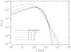 |
Fig. 1 κ-distributions for κ = 2, 3, 5, and 10 plotted with the Maxwellian distribution. Temperature of log T (K) = 6.5 is assumed. |
2. Method
2.1. Non-Maxwellian κ-distributions
The κ-distribution (Fig. 1) is a distribution of electron energies characterized by a power-law high-energy tail (Livadiotis & McComas 2009; Owocki & Scudder 1983),  (1)where Aκ is a normalization constant, kB is the Boltzmann constant, and T and κ are the parameters of the distribution. The free parameter κ changes the shape of distribution function from κ → 3/2, which corresponds to the highest deviation from Maxwellian distribution to κ → ∞, which corresponds to the Maxwellian distribution.
We note that the κ-distribution characterized by a parameter T can be approximated with a Maxwellian core with temperature TC = T(κ − 3/2) /κ and a power-law high-energy tail (Oka et al. 2013). Despite this, the mean energy ⟨E⟩ = 3kBT/ 2 of a κ-distribution is independent of κ, so that T can also be defined as the temperature for κ-distributions. Livadiotis & McComas (2009) showed that T has all the properties of the temperature in the generalized Tsallis statistical mechanics. Therefore, quantities depending on T, such as the pressure, internal energy, or the DEM(T) (Sect. 2.4), are straightforward to generalize for κ-distributions.
2.2. Synthetic spectra for κ-distributions
We assume that the solar corona is optically thin (e.g., Phillips et al. 2008). The intensity Iji of a spectral line with a wavelength λji that arises due to a transition j → i is given by the sum of all contributions from the plasma along the line of sight dl:  (2)where the contribution function Gji(T,Ne,κ) includes all atomic processes that contribute to the line formation. In optically thin conditions, it can be expressed as
  (3)In this expression, Aji is the Einstein coefficient giving the probability of the spontaneous emission, h is the Planck constant, c is the speed of light, Ne and NH are the electron and hydrogen densities, respectively,
  is the density of the k-times ionized ion of the element X with the electron on the excited upper level j,
  is the total density of the ion + k, and NX is the total density of the element X. The quantity
  represents the excited fraction of the ion + k. The
  is the relative ion abundance, and finally, AX = NX/NH is the abundance of the element X.
For evaluating the Gji(T,Ne,κ), the ionization equilibrium (i.e., the ) and the excitation equilibrium (i.e., the ) must be known. Usually, these are obtained by integrating the appropriate cross-sections for collisional ionization, recombination, excitation, and de-excitation over the Maxwellian distribution, as done in the CHIANTI database (Landi et al. 2013; Dere et al. 1997). However, the Gji(T,Ne,κ) can also be evaluated for the κ-distributions. Generally, the changes in Gji(T,Ne,κ) with κ are dominated by the ionization equilibrium, which exhibits wider and flatter ionization peaks, that can also be shifted to higher or lower temperatures (Dzifčáková & Dudík 2013; Dzifčáková 2002). Here, we use the ionization equilibrium calculations of Dzifčáková & Dudík (2013).
Changes in the electron collisional excitation and deexcitation rates and, therefore, in the excitation equilibrium, depend on the type of transitions and ratio of excitation energies to temperature. They can be calculated directly from atomic cross-sections, or, if the cross-sections are lacking, by using a method described in Dzifčáková (2006) and tested in Dzifčáková & Mason (2008). This is the approach we adopt here in conjunction with the atomic data from the CHIANTI database v7.1 (Landi et al. 2013). We also assume coronal abundances of Feldman et al. (1992) and constant pressure NeT = 1015 cm-3 K for both Maxwellian and non-Maxwellian calculations. Coronal abundances are required for an adequate description of the active region cores, which exhibit enhancements of the low-FIP elements by about a factor of three (e.g., Del Zanna 2013b; Del Zanna & Mason 2003). The assumption of constant pressure is justified on grounds of the maximum height of the loops in the active region cores being much lower than the pressure scale-height for temperatures of log T (K) ≈ 6.6 which are typical of active region cores. The lines used for the calculation of DEM are also typically not strongly sensitive to Ne, yielding little variation of the resulting DEM with the input value of NeT.
We also note here that we are not concerned in this paper with the effects of finite density on the ionization equilibrium or the possible presence of the transient (time-dependent) ionization. The reasons are as follows. First, while the suppression of dielectronic recombination at high Ne (e.g., Nikolić et al. 2013; Summers et al. 2006) leads to shifts of the ionization peaks toward lower T, this effect is typically small at the temperatures corresponding to active region cores even for log Ne (cm-3) = 10 (Fig. 6 in Nikolić et al. 2013). The effect of κ-distributions on the ionization equilibrium can be much stronger. Second, active region cores typically exhibit only weak intensity fluctuations even on timescales of several hours (e.g., Dudík et al. 2011a; Brooks & Warren 2009; Antiochos et al. 2003) indicating plasma near equilibrium. Therefore, we believe that the presence of plasmas undergoing transient ionization (cf. Doyle et al. 2013) can be neglected.
2.3. Response of the AIA 94 Å channel for κ-distributions
A procedure similar to the one outlined in Sect. 2.2 is used to obtain the responses of the AIA 94 Å channel for κ-distributions. The difference here is that the Gji(T,Ne,κ) for lines contributing to the AIA 94 Å channel were folded through the AIA 94 Å wavelength response, which is available from SolarSoft, to obtain the predicted intensities.
We used this procedure for the Fe xviii 93.93 Å line and the Fe xx 93.78 Å line. Note that the Fe xx line has usually a negligible contribution for active region conditions (O’Dwyer et al. 2010). We use the response of the AIA 94 Å emission calculated in this way, which is to exclude the contribution from cooler lines, such as Fe xiv and Fe x, because of the “cleaned” Fe xviii emission used by Warren et al. (2012) (see also Sect. 3). We also note that the Warren et al. (2012) method of obtaining the “cleaned” Fe xviii emission from AIA data appears reliable, since it gives nearly identical results to the method of Del Zanna (2013b), who take careful account of the lines contributing to the AIA 94 Å channel.
2.4. Differential emission measure analysis
Since the solar corona is optically thin, the line of sight l pierces plasma elements with different T and Ne. In principle, Eq. (2) can be re-cast as an integral over T and Ne (e.g., Phillips et al. 2008, p. 95 therein)  (4)where the ψ(T,Ne) is the emission measure differential. It can be considered to be a measure of the emission from the plasmas as a function of T and Ne. (Note that we do not consider here the possible dependence of ψ on κ for the reasons of simplicity.) Since the sensitivity of the contribution function Gji(T,Ne,κ) to Ne is usually weak compared to its sensitivity to T, the inversion of Eq. (4) in the density direction does not produce reliable results. Therefore, the quantity ψ(T,Ne) is typically reduced to the emission measure differential in temperature, DEM(T), which is also called the differential emission measure (DEM) and defined by (e.g., Phillips et al. 2008)
 ![Mathematical equation: \begin{equation} {\rm DEM}(T)=N_\mathrm{e}^2\frac{\mathrm{d}l}{\mathrm{d}T} \hspace{3cm} [\mathrm{cm^{-5}\,K^{-1}}] . \\ \label{Eq:def_DEM} \end{equation}](/articles/aa/full_html/2014/04/aa23054-13/aa23054-13-eq45.png) (5)The observed line intensity can then be written using Eqs. (2) and (5) as
(5)The observed line intensity can then be written using Eqs. (2) and (5) as  (6)The value of DEM(T) can be determined from an observed spectra by the inversion of Eq. (6) using a known set of Gji(T,Ne,κ) functions and an assumption on Ne, which assumes of constant pressure made in Sect. 2.2.
However, such inversion poses several problems with the uniqueness of its solutions. Therefore, many techniques have been developed to carry it out (Aschwanden & Boerner 2011; Goryaev et al. 2010; Golub et al. 2004; Weber et al. 2004; Parenti et al. 2000; Kashyap & Drake 1998; Brosius et al. 1996; Monsignori-Fossi & Landini 1992; Thompson 1990). One of the first used methods, the Withbroe-Sylwester (W-S) method (Sylwester et al. 1980; Withbroe 1975), and one of the most robust methods, the regularization method (RIM, Hannah & Kontar 2012), are employed in this paper to independently verify results.
The W-S method for DEM reconstruction was introduced by Withbroe (1975) and improved and tested by Sylwester et al. (1980). It was compared to other methods for the calculation of DEM (e.g., Siarkowski et al. 2008; Fludra & Sylwester 1986) and applied on solar data (e.g., Sylwester et al. 2010). The (n + 1)th approximation of a DEM model is given by  (7)where
  is the observed intensity in the line λji and
  is the intensity predicted in the nth iteration. The weight functions Wji(T) are chosen semi-empirically (see Eq. (12) in Sylwester et al. 1980) to improve the model most efficiently at temperatures where the line λji is formed. The initial approximation is DEM(0)(T) = const.
Hannah & Kontar (2012) present the RIM, which uses Tihkonov regularized inversion (Prato et al. 2006; Craig 1977; Tikhonov 1963) and generalized singular value decomposition (GSVD; Hansen 1992). The DEM is the solution of inversion of linearized equations system. The detailed explanation of RIM is presented in Hannah & Kontar (2012) and references therein. These authors also compared their RIM with commonly used Markov chain Monte Carlo (MCMC) method (Kashyap & Drake 1998) and have shown a good match to these two methods using data of an active region core from Warren et al. (2011). However, the RIM is computationally faster, provides error bars also in temperature, and the regularized solution matrix allows us to easily determine the accuracy and robustness of the regularized DEM.
3. Datasets selected for DEM reconstruction
To study the influence of κ-distributions on the DEM reconstruction, we used the data of Warren et al. (2012) and Landi & Young (2010). These observations were obtained using the Extreme Ultraviolet Imaging Spectrometer (EIS) onboard the Hinode satellite (Kosugi et al. 2007; Culhane et al. 2007) and the Atmospheric Imaging Assembly (AIA) onboard the Solar Dynamics Observatory (SDO; Pesnell et al. 2012; Lemen et al. 2012). The EIS observes EUV spectra in two spectral bands, 170–210 Å and 240–290 Å, with a spectral resolution 0.022 Å. Its spectral range contains emission lines providing sufficient coverage of the 0.6–5 MK temperature range. The “cleaned” emission of Fe xviii (Warren et al. 2012) observed by the AIA 94 Å channel is used to constrain the DEM at high temperatures above 5 MK.
Warren et al. (2012) selected 15 observations of inter-moss regions in active regions cores. The distribution of temperatures in such locations can constrain the properties of the coronal heating mechanism. For example, the slope of the DEM at temperatures lower than the DEM peak indicates whether the impulsive heating recurs on timescales longer or shorter than the typical plasma cooling time (see Winebarger 2012; Viall & Klimchuk 2011; Mulu-Moore et al. 2011; Tripathi et al. 2011). If the heating is high-frequency, in that it recurs often, the plasma cannot cool down. This is reflected on the DEM, which is strongly peaked, indicating plasma not far from equilibrium. This is what was found by Warren et al. (2012): The emission measure (EM) distributions, defined as  (8)are indeed strongly peaked in the active region cores. The EM(T) portions shortward of its peak were found to behave approximately as Tα with slopes α ≳ 2. The high-temperature portions of the EM(T) decrease as T− β with an even steeper β ≈ 5–15.
In this work, we reanalyze three typical regions out of the 15 observed by Warren et al. (2012). These are regions 5, 8, and 14. We selected these regions because of their different low-temperature slopes α. Region 5 represents a region with one of the lowest α found, which is ≈2. Region 8 is a region with an intermediate α, and finally, region 14 has the highest α = 4.8 ± 0.44. Warren et al. (2012) provides a list of calibrated data, which consists of intensities of 22 spectral lines observed by EIS and 1 intensity of AIA 94 channel of extracted box in 15 active regions. We estimate the typical uncertainties of observed intensities to be ≈30% (Hannah & Kontar 2012, Kontar; priv. comm.). These contain the calibration error, which is at least 10% (Wang et al. 2011) or higher (Del Zanna 2013a), atomic data errors, and errors arising from photon statistics. We note here that the RIM is still able to recover the DEM even if the calibration error is higher (Hannah & Kontar 2012). The list of used spectral lines with their observed intensities is given in Table 1. Note again that the estimated error of observed intensities is 30% and is not listed in Table 1.
 |
Fig. 2 EM-loci plots (different colors stand for different ions) and the EM distributions for inter-moss region 5 using the W-S method (light blue line) and the RIM (thick black line). The RIM provide vertical and horizontal error bars. The EM(T) for Maxwellian distribution (top left) and κ-distribution with κ = 5 (top right), κ = 3 (bottom left), κ = 2 (bottom right) is shown. The slopes of EMs are indicated by dark blue linear fits. The power-law indexes α and β are listed. |
 |
Fig. 3 Calculated-to-observed intensities IDEM/Iobs for the DEM reconstructions of region 5 under the assumption of Maxwellian and κ = 5, 3, and 2 distributions. Light blue squares are for W-S method. Color points with error bars are for RIM. Color coding is the same as in Fig. 2. The horizontal dashed lines represent the 30% error of observed intensities. |
Landi & Young (2010) present a list of intensities of a quiet Sun (QS) region above the west limb observed by the Hinode/EIS instrument on 2007 April 13. We used these data to complement the analysis of the active region cores. The list of used spectral lines with their observed intensities is given in Table 4 for data by Landi & Young (2010). Note that these lines are formed in a rather narrow range of temperatures (Landi & Young 2010).
4. Results
In general, it can be expected that the changes in Gji(T,Ne,κ) with κ-distributions could be reflected in the reconstructed DEMs. However, it is by no means a priori clear whether the reconstructed DEMs should become broader with κ, as do the individual Gji(T,Ne,κ) (see Sect. 2.2), or whether the DEMs may become more isothermal if the individual EM-loci curves, which are defined as  , shift toward a common crossing point.
To obtain an answer to this question, we use the W-S method and RIM in conjunction with the calculated Gji(T,Ne,κ) to reconstruct the DEMs for the selected datasets described in the previous section. To our knowledge, this is the first use of the DEM reconstruction methods for non-Maxwellian distributions.
List of spectral lines used in reconstruction of DEM by W-S method and RIM with the values of Iobs, RMaxw, and Rκ = 2 are shown for inter-moss region 5.
4.1. Active regions
The reconstructed DEMs are converted to the EM(T) using Eq. (8) and are shown in Fig. 2 for region 5, Fig. 4 for the region 8, and Fig. 6 for the region 14. In each one of these figures, the results are shown for the Maxwellian distribution with κ-distributions with κ = 5, 3, and 2. Note that these figures also contain the EM-loci plots, which represent upper limits for the reconstructed EM(T). The EM-loci plots are color-coded so that lines belonging to a particular element can be discerned at a glance. The results obtained from the RIM are plotted only for temperatures, where the DEMs were recovered reliably, specifically, where the resulting regularized solution matrix was almost diagonal. In contrast to that, the W-S method, which does not provide the errors in T, is plotted for the entire temperature range.
The DEMs recovered for the Maxwellian distribution are similar to those of Warren et al. (2012), which are calculated by the MCMC method. This similarity is expected, given that RIM and MCMC method give consistent results (Hannah & Kontar 2012).
The DEMs recovered under the assumption of a κ-distribution indicate similar behavior of the DEM with κ for all three regions investigated. With decreasing κ or increasing departures from the Maxwellian distribution, the DEM peaks become more rotund (concave). Furthermore, while the Maxwellian DEMs peak near log T (K) = 6.6 (≈4 MK), the temperatures corresponding to DEM peaks for κ are shifted to a higher temperatures, reaching log T (K) ~ 6.7–6.8 for κ = 2. These temperatures are about ≈1 MK higher than for the Maxwellian distribution. The shift of the DEM peaks can be attributed to the behavior of ionization equilibrium with κ, where the ionization peaks of the coronal ions (ions formed at log T (K) ≳ 6) are typically shifted to higher T. This is also illustrated in Fig. 8, where we plot the product of the Gji(T,Neκ) times EM(T) for some of the observed lines. For low κ = 2, the lines are formed at higher T and in broader range of temperatures.
 |
Fig. 8 G(T,ne,κ) × EM(T) for the Maxwellian (solid lines) and for the κ-distributions with κ = 2 (dashed lines) for indicated lines formed in different temperature ranges for region 5 (top), region 8 (middle), and region 14 (bottom). The EM(T) is calculated by W-S method. |
Note that it is not surprising that the DEM peaks are found at around log T (K) = 6.6 for the Maxwellian distribution (compare with Wood & Laming 2013) and at slightly higher log T (K) for lower κ. Such temperatures correspond well to the minima of the radiative loss function for different κ (Dudík et al. 2011b). Even if the plasma is heated to higher T, radiative losses are least efficient at the temperatures corresponding to the minima of the radiative loss function.
Generally, we find a good agreement between the DEMs recovered using the RIM and W-S method. However, the RIM underestimates the peak emission and smooths it in comparison with the W-S method. This is due to several reasons. First, the errors of the input intensities Iobs are large, ≈30% (Sect. 3), and the behavior of the RIM for such cases is known (Hannah & Kontar 2012). In essence, large uncertainties in the EM-loci plots prevent the RIM from recovering sharply peaked DEMs, even if the plasma is truly isothermal. Second, the RIM tries to recover the DEM under the constraint of smallest total emission measure possible.
We perform fitting of both the low-temperature and high-temperature slopes of the recovered EM(T). These fits are also shown in Figs. 2–6, and the appropriate values of the slopes α and β are also listed in these figures. We find that the value of α does not change appreciably with κ, while the value of β is generally somewhat lower for lower κ. This is due to the rotundness of the EM peaks for low κ. We conclude that the assumption of a κ-distribution in DEM reconstruction does not significantly change the constraints on the coronal heating problem drawn from the steepness of the EM(T) slopes.
As already noted, the Maxwellian DEM for region 5 is much more multithermal than the one for region 14. The obtained consistent behavior of the reconstructed DEMs with κ for all three regions and two different DEM reconstruction methods establishes confidence in the reconstructed DEMs for the κ-distributions.
The ratios R of the observed and calculated intensities, R = IDEM/Iobs, are for the three regions, the Maxwellian and κ = 2 distributions listed in Tables 1–3. The IDEM were calculated using W-S method and RIM. The ratios indicate the ability of the reconstructed DEMs to reproduce the observed intensities. Values of R within 0.7 <R< 1.3 mean that IDEM is within 30% of the estimated error of observed intensities. The relative error χ of reconstructed DEM, as calculated from  , are in the last row of Tables 1–3. For the W-S method, the χ is slightly better for Maxwellian distribution than for κ = 2. For RIM, they are 30% irrespective of the distribution.
The calculated-to-observed intensities R for both methods are also graphically presented in Figs. 3, 5, and 7. For RIM, errors of the DEM(T) are propagated to obtain the errors σ(IDEM) of the reconstructed intensities. These are shown as error bars for the corresponding R values. The ratios are typically within the interval 0.7 <R< 1.3. Exceptions are ratios for lines formed at temperatures corresponding to the DEM peak. This is caused by the inability of the methods to exactly recover sharply peaked DEMs. Finally, we note that this type of error analysis is designed only to determine the goodness-of-fit for individual lines. It is not designed to determine which type of distribution and its corresponding DEM offer a better approximation for all of the observed intensities. These observed lines are not sufficient for diagnostics of κ either (Dzifčáková & Kulinová 2010; Mackovjak et al. 2013).
4.2. Quiet Sun
List of spectral lines from Landi & Young (2010) used in the reconstruction of DEM by W-S method and RIM. The Iobs, RMaxw, and Rκ = 2 are shown.
The DEM reconstruction is also performed on the quiet Sun data of Landi & Young (2010), and the results are presented in terms of EM(T) in Fig. 9. For the Maxwellian distribution, the EM(T) peaks at log T (K) = 6.15 (1.4 MK). This is in good agreement with the results of Landi & Young (2010), although they used another iterative technique developed by Landi & Landini (1997) to determine the DEM. Note that outside of log T (K) ~ 6.0–6.3 for the Maxwellian distribution, the regularized solution matrix was clearly not diagonal, producing large horizontal errors. This means that the DEM calculated by the RIM is not reliable at these temperatures and is again not displayed.
For κ-distributions, the EM(T) peak is again shifted progressively to higher T, reaching log T (K) ≈ 6.3 (2 MK) for κ = 2. Note that while the EM-loci plots indicate multithermal plasma for the Maxwellian distribution, they indicate progressively less multithermal plasma for lower κ. Especially for κ = 2, the EM-loci curves nearly intersect at a common point (Fig. 9, bottom right). Consequently, it is possible to interpret the same observed spectrum either as emission from multithermal plasma with a narrow DEM and Maxwellian distribution, or as emission from near-isothermal plasma with κ = 2. Indeed, upon fitting the EM slopes, we find that the value of α progressively increases from 3.66 ± 0.15 for the Maxwellian distribution to 5.77 ± 0.31 for κ = 2. It is, however, not clear what coronal heating mechanism could produce such extremely non-Maxwellian distributions in the quiet Sun.
The ratios R of the calculated-to-observed intensities, R = IDEM/Iobs, are presented in Table 4. The IDEM were calculated using W-S method and RIM. The plots of the calculated-to-observed intensities ratios are shown in Fig. 10.
 |
Fig. 9 DEM for quiet Sun region using W-S method (light blue line) and the RIM (thick black line). The constant pressure log pe (cm-3 K) = 15 is assumed. The RIM provide vertical and horizontal error bars. The DEM for Maxwellian distribution (top left) and κ-distribution with κ = 5 (top right), κ = 3 (bottom left), κ = 2 (bottom right) is shown. The slope of DEM is indicated by the dark blue linear fit and appropriate power-law indexes (parameter α indicates the slope of increasing DEM peak and β indicates the negative slope of decreasing DEM peak). Correspondent EM-loci curves are also shown, and they are color-coded by ion. |
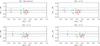 |
Fig. 10 Calculated-to-observed intensities for the quiet Sun region, assuming Maxwellian distribution and κ-disribution with κ = 5, 3, and 2. Light blue squares are for W-S method. Color points with error bars are for RIM, and the color coding is the same as in the Fig. 9. Two horizontal dashed lines represent the error of observed intensities, which are at 30%. |
5. Conclusions and outlook
We have investigated the temperature structure of several active region cores and a quiet Sun region under the assumption of the non-Maxwellian κ-distributions. To recover the differential emission measure, we used two methods, namely the Withbroe-Sylwester method and the regularization method. Our main results can be summarized as follows:
-
Both DEM reconstruction methods give similar solutions. Thisgives confidence in the validity of the reconstructed DEMs.
-
The reconstructed Maxwellian DEMs for three active region cores and quiet Sun region are in good qualitative agreement with results published by other authors, who use different DEM reconstruction techniques.
-
The influence of κ-distributions on the DEMs is similar for each of the three active region cores studied. With decreasing κ, the DEMs become more rotund and their peaks are shifted to higher temperatures. This is chiefly a consequence of changes in ionization equilibrium, which also cause individual lines to be formed at a wider range of temperatures.
-
The slopes of the EM distributions leftward of its peak do not change appreciably with κ. This suggests that different assumptions on the shape of the electron distribution function do not change the constraints on the coronal heating mechanism.
-
Interpretation of quiet Sun plasma emission may differ for different types of electron distribution assumed. The DEM is found to be multithermal for Maxwellian distribution, but is much less multithermal for κ ≈ 2.
In summary, our results show that the multithermality of plasma can be a robust result, although the degree of the multithermality is dependent on the region observed and assumed particle distribution. Especially in the active region cores, some constraints on the coronal heating can be derived from DEM reconstruction regardless of the particle microphysics. For example, the relative number of high-energy electrons produced by the coronal heating. This is a somewhat surprising result, since the contribution functions of the individual spectral lines are highly dependent on the assumed distribution function.
This dependency of the contribution functions on the distribution of particle energies calls for a closer scrutiny of the spectroscopic observations. A positive diagnostics of the non-Maxwellian distributions in the solar corona would be a “smoking gun” for the coronal heating process involved and could possibly help explain the source of the solar wind. Unfortunately, the present spectroscopic observations have limited wavelength coverages and often suffer from instrument and calibration issues preventing the diagnostics (see Mackovjak et al. 2013; Del Zanna 2013a), as well as atomic data uncertainties. A comprehensive search for lines suitable for diagnostics of non-Maxwellian distributions in the entire wavelength range is planned. This is of importance for the interpretation of current and future observations and could also result in improved instrument design. In the meantime, the results presented here shed a new light on the long-standing issue of isothermal vs. multithermal plasma.
Acknowledgments
The authors are grateful to prof. Janusz Sylwester for providing the IDL code for the W-S method and to Dr. Eduard Kontar for helpful discussions about RIM. The authors are also thankful to the referee for the remarks that led to improvements of the manuscript. This work was supported by the grant No. 209/12/1652 of the Grant Agency of the Czech Republic and the Bilateral Project CZ-SK-0153-11. ŠM acknowledges Comenius University grant No. UK/387/2013. JD acknowledges support from the Royal Society via the Newton Fellowships Programme. The authors are also thankful for the support provided by the International Space Science Institute through its International Teams program. Hinode is a Japanese mission developed and launched by ISAS/JAXA, with NAOJ as domestic partner and NASA and STFC (UK) as international partners. It is operated by these agencies in cooperation with ESA and NSC (Norway). CHIANTI is a collaborative project involving the NRL (USA), the University of Cambridge (UK) and George Mason University (USA).
References
- Antiochos, S. K., Karpen, J. T., DeLuca, E. E., Golub, L., & Hamilton, P. 2003, ApJ, 590, 547 [NASA ADS] [CrossRef] [Google Scholar]
- Aschwanden, M. J., & Boerner, P. 2011, ApJ, 732, 81 [NASA ADS] [CrossRef] [Google Scholar]
- Aschwanden, M. J., Nitta, N. V., Wuelser, J.-P., & Lemen, J. R. 2008, ApJ, 680, 1477 [NASA ADS] [CrossRef] [Google Scholar]
- Brooks, D. H., & Warren, H. P. 2009, ApJ, 703, L10 [NASA ADS] [CrossRef] [Google Scholar]
- Brooks, D. H., Warren, H. P., & Young, P. R. 2011, ApJ, 730, 85 [NASA ADS] [CrossRef] [Google Scholar]
- Brooks, D. H., Warren, H. P., & Ugarte-Urra, I. 2012, ApJ, 755, L33 [NASA ADS] [CrossRef] [Google Scholar]
- Brosius, J. W., Davila, J. M., Thomas, R. J., & Monsignori-Fossi, B. C. 1996, ApJS, 106, 143 [NASA ADS] [CrossRef] [Google Scholar]
- Cirtain, J. W., Golub, L., Winebarger, A. R., et al. 2013, Nature, 493, 501 [NASA ADS] [CrossRef] [Google Scholar]
- Collier, M. R., Hamilton, D. C., Gloeckler, G., Bochsler, P., & Sheldon, R. B. 1996, Geophys. Res. Lett., 23, 1191 [NASA ADS] [CrossRef] [Google Scholar]
- Craig, I. J. D. 1977, A&A, 61, 575 [NASA ADS] [Google Scholar]
- Craig, I. J. D., & Brown, J. C. 1976, A&A, 49, 239 [NASA ADS] [Google Scholar]
- Culhane, J. L., Harra, L. K., James, A. M., et al. 2007, Sol. Phys., 243, 19 [Google Scholar]
- DeForest, C. E. 2007, ApJ, 661, 532 [NASA ADS] [CrossRef] [Google Scholar]
- Del Zanna, G. 2013a, A&A, 555, A47 [NASA ADS] [CrossRef] [EDP Sciences] [Google Scholar]
- Del Zanna, G. 2013b, A&A, 558, A73 [NASA ADS] [CrossRef] [EDP Sciences] [Google Scholar]
- Del Zanna, G., & Mason, H. E. 2003, A&A, 406, 1089 [NASA ADS] [CrossRef] [EDP Sciences] [Google Scholar]
- Del Zanna, G., O’Dwyer, B., & Mason, H. E. 2011, A&A, 535, A46 [NASA ADS] [CrossRef] [EDP Sciences] [Google Scholar]
- Dere, K. P., Landi, E., Mason, H. E., Monsignori Fossi, B. C., & Young, P. R. 1997, A&AS, 125, 149 [NASA ADS] [CrossRef] [EDP Sciences] [Google Scholar]
- Dialynas, K., Krimigis, S. M., Mitchell, D. G., et al. 2009, J. Geophys. Res., 114, 1212 [Google Scholar]
- Doyle, J. G., Giunta, A., Madjarska, M. S., et al. 2013, A&A, 557, L9 [NASA ADS] [CrossRef] [EDP Sciences] [Google Scholar]
- Dudík, J., Kulinová, A., Dzifčáková, E., & Karlický, M. 2009, A&A, 505, 1255 [NASA ADS] [CrossRef] [EDP Sciences] [Google Scholar]
- Dudík, J., Dzifčáková, E., Karlický, M., & Kulinová, A. 2011a, A&A, 531, A115 [NASA ADS] [CrossRef] [EDP Sciences] [Google Scholar]
- Dudík, J., Dzifčáková, E., Karlický, M., & Kulinová, A. 2011b, A&A, 529, A103 [NASA ADS] [CrossRef] [EDP Sciences] [Google Scholar]
- Dzifčáková, E. 2002, Sol. Phys., 208, 91 [NASA ADS] [CrossRef] [Google Scholar]
- Dzifčáková, E. 2006, in SOHO-17. 10 Years of SOHO and Beyond, ESA SP, 617 [Google Scholar]
- Dzifčáková, E., & Dudík, J. 2013, ApJS, 206, 6 [NASA ADS] [CrossRef] [Google Scholar]
- Dzifčáková, E., & Kulinová, A. 2010, Sol. Phys., 263, 25 [NASA ADS] [CrossRef] [Google Scholar]
- Dzifčáková, E., & Kulinová, A. 2011, A&A, 531, A122 [NASA ADS] [CrossRef] [EDP Sciences] [Google Scholar]
- Dzifčáková, E., & Mason, H. 2008, Sol. Phys., 247, 301 [NASA ADS] [CrossRef] [Google Scholar]
- Feldman, U., Mandelbaum, P., Seely, J. F., Doschek, G. A., & Gursky, H. 1992, ApJS, 81, 387 [NASA ADS] [CrossRef] [Google Scholar]
- Feldman, U., Landi, E., & Doschek, G. A. 2007, ApJ, 660, 1674 [NASA ADS] [CrossRef] [Google Scholar]
- Fludra, A., & Sylwester, J. 1986, Sol. Phys., 105, 323 [NASA ADS] [CrossRef] [Google Scholar]
- Golub, L., Deluca, E. E., Sette, A., & Weber, M. 2004, in The Solar-B Mission and the Forefront of Solar Physics, eds. T. Sakurai, & T. Sekii, ASP Conf. Ser., 325, 217 [Google Scholar]
- Goryaev, F. F., Parenti, S., Urnov, A. M., et al. 2010, A&A, 523, A44 [NASA ADS] [CrossRef] [EDP Sciences] [Google Scholar]
- Hannah, I. G., & Kontar, E. P. 2012, A&A, 539, A146 [NASA ADS] [CrossRef] [EDP Sciences] [Google Scholar]
- Hansen, P. C. 1992, Inverse Problems, 8, 849 [NASA ADS] [CrossRef] [Google Scholar]
- Judge, P. G., Hubeny, V., & Brown, J. C. 1997, ApJ, 475, 275 [NASA ADS] [CrossRef] [EDP Sciences] [Google Scholar]
- Kashyap, V., & Drake, J. J. 1998, ApJ, 503, 450 [NASA ADS] [CrossRef] [Google Scholar]
- Kašparová, J., & Karlický, M. 2009, A&A, 497, L13 [NASA ADS] [CrossRef] [EDP Sciences] [Google Scholar]
- Kletzing, C. A., Scudder, J. D., Dors, E. E., & Curto, C. 2003, J. Geophys. Res., 108, 1360 [CrossRef] [Google Scholar]
- Kosugi, T., Matsuzaki, K., Sakao, T., et al. 2007, Sol. Phys., 243, 3 [NASA ADS] [CrossRef] [Google Scholar]
- Landi, E., & Landini, M. 1997, A&A, 327, 1230 [NASA ADS] [Google Scholar]
- Landi, E., & Young, P. R. 2010, ApJ, 714, 636 [NASA ADS] [CrossRef] [Google Scholar]
- Landi, E., Young, P. R., Dere, K. P., Del Zanna, G., & Mason, H. E. 2013, ApJ, 763, 86 [NASA ADS] [CrossRef] [Google Scholar]
- Lanzafame, A. C., Brooks, D. H., Lang, J., et al. 2002, A&A, 384, 242 [NASA ADS] [CrossRef] [EDP Sciences] [Google Scholar]
- Lanzafame, A. C., Brooks, D. H., & Lang, J. 2005, A&A, 432, 1063 [NASA ADS] [CrossRef] [EDP Sciences] [Google Scholar]
- Le Chat, G., Issautier, K., Meyer-Vernet, N., & Hoang, S. 2011, Sol. Phys., 271, 141 [NASA ADS] [CrossRef] [Google Scholar]
- Lee, E., Williams, D. R., & Lapenta, G. 2013, A&A [arXiv:1305.2939] [Google Scholar]
- Lemen, J. R., Title, A. M., Akin, D. J., et al. 2012, Sol. Phys., 275, 17 [NASA ADS] [CrossRef] [Google Scholar]
- Leubner, M. P. 2002, Ap&SS, 282, 573 [NASA ADS] [CrossRef] [Google Scholar]
- Leubner, M. P. 2004, Phys. Plasmas, 11, 1308 [NASA ADS] [CrossRef] [Google Scholar]
- Livadiotis, G., & McComas, D. J. 2009, J. Geophys. Res., 114, 11105 [Google Scholar]
- Livadiotis, G., & McComas, D. J. 2010, ApJ, 714, 971 [NASA ADS] [CrossRef] [Google Scholar]
- Livadiotis, G., & McComas, D. J. 2013, Space Sci. Rev., 175, 183 [NASA ADS] [CrossRef] [Google Scholar]
- Mackovjak, Š., Dzifčáková, E., & Dudík, J. 2013, Sol. Phys., 282, 263 [NASA ADS] [CrossRef] [Google Scholar]
- Maksimovic, M., Pierrard, V., & Riley, P. 1997, Geophys. Res. Lett., 24, 1151 [NASA ADS] [CrossRef] [Google Scholar]
- Monsignori-Fossi, B. C., & Landini, M. 1992, Mem. Soc. Astron. It., 63, 767 [NASA ADS] [Google Scholar]
- Mulu-Moore, F. M., Winebarger, A. R., & Warren, H. P. 2011, ApJ, 742, L6 [NASA ADS] [CrossRef] [Google Scholar]
- Nikolić, D., Gorczyca, T. W., Korista, K. T., Ferland, G. J., & Badnell, N. R. 2013, ApJ, 768, 82 [NASA ADS] [CrossRef] [Google Scholar]
- O’Dwyer, B., Del Zanna, G., Mason, H. E., Weber, M. A., & Tripathi, D. 2010, A&A, 521, A21 [NASA ADS] [CrossRef] [EDP Sciences] [Google Scholar]
- O’Dwyer, B., Del Zanna, G., Mason, H. E., et al. 2011, A&A, 525, A137 [NASA ADS] [CrossRef] [EDP Sciences] [Google Scholar]
- Oka, M., Ishikawa, S., Saint-Hilaire, P., Krucker, S., & Lin, R. P. 2013, ApJ, 764, 6 [NASA ADS] [CrossRef] [Google Scholar]
- Owocki, S. P., & Scudder, J. D. 1983, ApJ, 270, 758 [NASA ADS] [CrossRef] [Google Scholar]
- Parenti, S., & Vial, J.-C. 2007, A&A, 469, 1109 [NASA ADS] [CrossRef] [EDP Sciences] [Google Scholar]
- Parenti, S., Bromage, B. J. I., Poletto, G., et al. 2000, A&A, 363, 800 [NASA ADS] [Google Scholar]
- Pesnell, W. D., Thompson, B. J., & Chamberlin, P. C. 2012, Sol. Phys., 275, 3 [NASA ADS] [CrossRef] [Google Scholar]
- Peter, H., Bingert, S., Klimchuk, J. A., et al. 2013, A&A, 556, A104 [NASA ADS] [CrossRef] [EDP Sciences] [Google Scholar]
- Phillips, K. J. H., Feldman, U., & Landi, E. 2008, Ultraviolet and X-ray Spectroscopy of the Solar Atmosphere (Cambridge University Press) [Google Scholar]
- Pierrard, V., & Lazar, M. 2010, Sol. Phys., 267, 153 [NASA ADS] [CrossRef] [Google Scholar]
- Pinfield, D. J., Keenan, F. P., Mathioudakis, M., et al. 1999, ApJ, 527, 1000 [NASA ADS] [CrossRef] [Google Scholar]
- Prato, M., Piana, M., Brown, J. C., et al. 2006, Sol. Phys., 237, 61 [NASA ADS] [CrossRef] [Google Scholar]
- Reale, F., Testa, P., Klimchuk, J. A., & Parenti, S. 2009, ApJ, 698, 756 [CrossRef] [Google Scholar]
- Schmelz, J. T., & Martens, P. C. H. 2006, ApJ, 636, L49 [NASA ADS] [CrossRef] [EDP Sciences] [Google Scholar]
- Schmelz, J. T., Nasraoui, K., Rightmire, L. A., et al. 2009, ApJ, 691, 503 [NASA ADS] [CrossRef] [Google Scholar]
- Schmelz, J. T., Jenkins, B. S., Worley, B. T., et al. 2011a, ApJ, 731, 49 [NASA ADS] [CrossRef] [Google Scholar]
- Schmelz, J. T., Worley, B. T., Anderson, D. J., et al. 2011b, ApJ, 739, 33 [NASA ADS] [CrossRef] [Google Scholar]
- Schmelz, J. T., Jenkins, B. S., & Pathak, S. 2013, ApJ, 770, 14 [NASA ADS] [CrossRef] [Google Scholar]
- Scudder, J. D., & Karimabadi, H. 2013, ApJ, 770, 26 [NASA ADS] [CrossRef] [Google Scholar]
- Shoub, E. C. 1983, ApJ, 266, 339 [NASA ADS] [CrossRef] [Google Scholar]
- Siarkowski, M., Falewicz, R., Kepa, A., & Rudawy, P. 2008, Ann. Geophys., 26, 2999 [NASA ADS] [CrossRef] [Google Scholar]
- Summers, H. P., Dickson, W. J., O’Mullane, M. G., et al. 2006, Plasma Phys. Control. Fusion, 48, 263 [CrossRef] [Google Scholar]
- Sylwester, J., Schrijver, J., & Mewe, R. 1980, Sol. Phys., 67, 285 [NASA ADS] [CrossRef] [Google Scholar]
- Sylwester, B., Sylwester, J., & Phillips, K. J. H. 2010, A&A, 514, A82 [NASA ADS] [CrossRef] [EDP Sciences] [Google Scholar]
- Thompson, A. M. 1990, A&A, 240, 209 [NASA ADS] [Google Scholar]
- Tikhonov, A. N. 1963, Sov. Math. Dokl., 4, 1035 [Google Scholar]
- Tripathi, D., Klimchuk, J. A., & Mason, H. E. 2011, ApJ, 740, 111 [NASA ADS] [CrossRef] [Google Scholar]
- Tsallis, C. 1988, J. Stat. Phys., 52, 479 [NASA ADS] [CrossRef] [MathSciNet] [Google Scholar]
- Tsallis, C. 2009, Introduction to Nonextensive Statistical Mechanics (Berlin, Heidelberg: Springer Verlag) [Google Scholar]
- Viall, N. M., & Klimchuk, J. A. 2011, ApJ, 738, 24 [Google Scholar]
- Wang, T., Thomas, R. J., Brosius, J. W., et al. 2011, ApJS, 197, 32 [NASA ADS] [CrossRef] [Google Scholar]
- Warren, H. P., Brooks, D. H., & Winebarger, A. R. 2011, ApJ, 734, 90 [NASA ADS] [CrossRef] [Google Scholar]
- Warren, H. P., Winebarger, A. R., & Brooks, D. H. 2012, ApJ, 759, 141 [NASA ADS] [CrossRef] [Google Scholar]
- Weber, M. A., Deluca, E. E., Golub, L., & Sette, A. L. 2004, in Multi-Wavelength Investigations of Solar Activity, eds. A. V. Stepanov, E. E. Benevolenskaya, & A. G. Kosovichev, IAU Symp., 223, 321 [Google Scholar]
- Winebarger, A. R. 2012, in Fifth Hinode Science Meeting, eds. L. Golub, I. De Moortel, & T. Shimizu, ASP Conf. Ser., 456, 103 [Google Scholar]
- Winebarger, A. R., Schmelz, J. T., Warren, H. P., Saar, S. H., & Kashyap, V. L. 2011, ApJ, 740, 2 [NASA ADS] [CrossRef] [Google Scholar]
- Winebarger, A. R., Warren, H. P., Schmelz, J. T., et al. 2012, ApJ, 746, L17 [NASA ADS] [CrossRef] [Google Scholar]
- Withbroe, G. L. 1975, Sol. Phys., 45, 301 [NASA ADS] [CrossRef] [Google Scholar]
- Wood, B. E., & Laming, J. M. 2013, ApJ, 768, 122 [NASA ADS] [CrossRef] [Google Scholar]
- Zouganelis, I. 2008, J. Geophys. Res., 113, 8111 [Google Scholar]
All Tables
List of spectral lines used in reconstruction of DEM by W-S method and RIM with the values of Iobs, RMaxw, and Rκ = 2 are shown for inter-moss region 5.
List of spectral lines from Landi & Young (2010) used in the reconstruction of DEM by W-S method and RIM. The Iobs, RMaxw, and Rκ = 2 are shown.
All Figures
|
Fig. 1 κ-distributions for κ = 2, 3, 5, and 10 plotted with the Maxwellian distribution. Temperature of log T (K) = 6.5 is assumed. |
| In the text | |
|
Fig. 2 EM-loci plots (different colors stand for different ions) and the EM distributions for inter-moss region 5 using the W-S method (light blue line) and the RIM (thick black line). The RIM provide vertical and horizontal error bars. The EM(T) for Maxwellian distribution (top left) and κ-distribution with κ = 5 (top right), κ = 3 (bottom left), κ = 2 (bottom right) is shown. The slopes of EMs are indicated by dark blue linear fits. The power-law indexes α and β are listed. |
| In the text | |
|
Fig. 3 Calculated-to-observed intensities IDEM/Iobs for the DEM reconstructions of region 5 under the assumption of Maxwellian and κ = 5, 3, and 2 distributions. Light blue squares are for W-S method. Color points with error bars are for RIM. Color coding is the same as in Fig. 2. The horizontal dashed lines represent the 30% error of observed intensities. |
| In the text | |
 |
Fig. 4 Same as Fig. 2 but for region 8. |
| In the text | |
 |
Fig. 5 Same as Fig. 3 but for region 8. |
| In the text | |
 |
Fig. 6 Same as Fig. 2 but for region 14. |
| In the text | |
 |
Fig. 7 Same as Fig. 3 but for region 14. |
| In the text | |
|
Fig. 8 G(T,ne,κ) × EM(T) for the Maxwellian (solid lines) and for the κ-distributions with κ = 2 (dashed lines) for indicated lines formed in different temperature ranges for region 5 (top), region 8 (middle), and region 14 (bottom). The EM(T) is calculated by W-S method. |
| In the text | |
|
Fig. 9 DEM for quiet Sun region using W-S method (light blue line) and the RIM (thick black line). The constant pressure log pe (cm-3 K) = 15 is assumed. The RIM provide vertical and horizontal error bars. The DEM for Maxwellian distribution (top left) and κ-distribution with κ = 5 (top right), κ = 3 (bottom left), κ = 2 (bottom right) is shown. The slope of DEM is indicated by the dark blue linear fit and appropriate power-law indexes (parameter α indicates the slope of increasing DEM peak and β indicates the negative slope of decreasing DEM peak). Correspondent EM-loci curves are also shown, and they are color-coded by ion. |
| In the text | |
|
Fig. 10 Calculated-to-observed intensities for the quiet Sun region, assuming Maxwellian distribution and κ-disribution with κ = 5, 3, and 2. Light blue squares are for W-S method. Color points with error bars are for RIM, and the color coding is the same as in the Fig. 9. Two horizontal dashed lines represent the error of observed intensities, which are at 30%. |
| In the text | |
Current usage metrics show cumulative count of Article Views (full-text article views including HTML views, PDF and ePub downloads, according to the available data) and Abstracts Views on Vision4Press platform.
Data correspond to usage on the plateform after 2015. The current usage metrics is available 48-96 hours after online publication and is updated daily on week days.
Initial download of the metrics may take a while.