| Issue |
A&A
Volume 564, April 2014
|
|
|---|---|---|
| Article Number | A100 | |
| Number of page(s) | 13 | |
| Section | Stellar structure and evolution | |
| DOI | https://doi.org/10.1051/0004-6361/201322988 | |
| Published online | 11 April 2014 | |
On the effect of rotation on populations of classical Cepheids
I. Predictions at solar metallicity
1
Observatoire de Genève, Université de Genève, 51 Chemin des Maillettes, 1290
Sauverny,
Switzerland
e-mail: This email address is being protected from spambots. You need JavaScript enabled to view it.
2
Astrophysics group, Lennard-Jones Laboratories, EPSAM, Keele
University, Staffordshire, ST5
5BG, UK
Received:
5
November
2013
Accepted:
6
February
2014
Abstract
Context. Classical Cepheids are among the most important variable star types due to their nature as standard candles and have a long history of modeling in terms of stellar evolution. The effects of rotation on Cepheids have not yet been discussed in detail in the literature, although some qualitative trends have already been mentioned.
Aims. We aim to improve the understanding of Cepheids from an evolutionary perspective and establish the role of rotation in the Cepheid paradigm. In particular, we are interested in the contribution of rotation to the problem of Cepheid masses, and explore testable predictions of quantities that can be confronted with observations.
Methods. Recently developed evolutionary models including a homogeneous and self-consistent treatment of axial rotation are studied in detail during the crossings of the classical instability strip (IS). The dependence of a suite of parameters on initial rotation is studied. These parameters include mass, luminosity, temperature, lifetimes, equatorial velocity, surface abundances, and rates of period change.
Results. Several key results are obtained: i) mass−luminosity (M − L) relations depend on rotation, particularly during the blue loop phase; ii) luminosity increases between crossings of the IS. Hence, Cepheid M − L relations at fixed initial rotation rate depend on crossing number (the faster the rotation, the larger the luminosity difference between crossings); iii) the Cepheid mass discrepancy problem vanishes when rotation and crossing number are taken into account, without a need for high core overshooting values or enhanced mass loss; iv) rotation creates dispersion around average parameters predicted at fixed mass and metallicity. This is of particular importance for the period−luminosity relation, for which rotation is a source of intrinsic dispersion; v) enhanced surface abundances do not unambiguously distinguish Cepheids occupying the Hertzsprung gap from ones on blue loops (after dredge-up), since rotational mixing can lead to significantly enhanced main sequence (MS) abundances; vi) rotating models predict greater Cepheid ages than non-rotating models due to longer MS lifetimes.
Conclusions. Rotation has a significant evolutionary impact on classical Cepheids and should no longer be neglected in their study.
Key words: stars: variables: Cepheids / supergiants / stars: evolution / stars: rotation / stars: abundances / distance scale
© ESO, 2014
1. Introduction
Classical Cepheids are objects of interest for many areas of astrophysics. On the one hand, they are excellent standard candles allowing the determination of distances in the Milky Way and up to Virgo cluster distances. On the other hand, they are excellent objects for constraining stellar evolutionary models. Accordingly, Cepheids have played a special role among pulsating (variable) stars and have a long history of modeling efforts both in terms of their evolution and pulsations (see Bono et al. 2013, and references therein).
Following the development of pulsation models in the late 1960s (Christy 1968; Stobie 1969a,b,c), systematic differences between pulsational and evolutionary masses of Cepheids became apparent. These differences were originally referred to as Cepheid mass anomalies (Cox 1980). Improved opacities (Iglesias & Rogers 1991; Seaton et al. 1994) could mitigate a good fraction of the disaccord in terms of masses. Nowadays, it is common to speak of the mass discrepancy as the systematic offset between evolutionary masses and those derived with other methods (e.g. Bono et al. 2006; Keller 2008), with a typical disagreement at the level of 10–20%.
Several mechanisms have been put forward to resolve the mass discrepancy problem. Among the most prominent in the recent literature are augmented convective core overshooting (Prada Moroni et al. 2012) and pulsation-enhanced mass-loss (Neilson & Lester 2008). However, the effect of rotation on evolutionary Cepheid masses has not been discussed in detail although the impact of rotation on the mass−luminosity and period−luminosity relations have already been mentioned previously in the literature (see Maeder & Meynet 2000, 2001).
The first large grid of models incorporating a homogeneous and consistent treatment of axial rotation was recently presented by Ekström et al. (2012, hereafter E12). Subsequently, Georgy et al. (2013, hereafter G13) extended the grid in terms of rotation for stars between 1.7 and 15 M⊙. Using these state-of-the-art grids it is now possible, for the first time, to consider the effect of rotation on populations of classical Cepheids.
Cepheid progenitors are B-type stars on the main sequence (MS). Observationally, B-type stars are known for their fast rotation since the first homogeneous study of rotational velocities by Slettebak (1949). Thus, it is empirically known that fast rotation is common for the progenitors of Cepheids. Huang et al. (2010) have recently carried out a very detailed investigation of rotational velocities for B-stars of different masses and evolutionary states (on the MS), providing even an empirical distribution of rotation rates. Their distribution can serve as a guideline for our study in the sense that the typical MS rotation rates of B-stars in the mass range appropriate for Cepheids (~5−9 M⊙) is approximately v/vcrit = 0.3−0.4, where vcrit denotes critical rotation velocity. As shown in E12 and G13, such fast rotation can significantly alter the evolutionary path of stars by introducing additional mixing effects that impact MS lifetime, stellar core size, age, and MS surface abundances. Clearly, these effects will propagate into the advanced stages of evolution, such as the Cepheid stage.
The blue loop phase of intermediate-mass evolved stars during core helium burning is very sensitive to the input physics (see the “magnifying glass” metaphor in Kippenhahn & Weigert 1994, p. 305). Thus, there is a two-fold interest in studying the models presented in E12 and G13 in terms of their predictions for Cepheids: i) properties of Cepheids inferred using models (e.g. mass) can be updated to account for rotation; ii) certain predictions made by the models can be tested immediately using observational data (e.g. surface abundances).
This paper is the first in a series devoted to the endeavor of extending the evolutionary paradigm of Cepheids to include the effects of rotation. We here focus mainly on the detailed exploration of predictions made by the models as well as their interpretation. A detailed comparison of these predictions to observed features is in progress and will be presented in a future publication for the sake of brevity. Further projects will include the investigation of the combined effect of metallicity and rotation as well as a self-consistent determination of pulsation periods and instability strip boundaries.
The structure of this paper is as follows. In Sect. 2, we briefly state a few key aspects of the models presented in E12 and G13 relevant in the context of this work. Section 3 contains the predictions made by the rotating Cepheid models, focusing on the mass discrepancy and features that are accessible to observations. Section 4 discusses the reliability and implications of the predictions made, and Sect. 5 summarizes the key aspects.
2. Description and comparison of input physics
The input physics of the stellar models are explained in detail in E12 and G13. We refer the reader to these publications for the detailed description of the models and summarize here only the most relevant features. The solar composition adopted is that by Asplund et al. (2005), and the detailed abundances of all elements are listed in E12.
Rotation is treated in the Roche model framework with the shellular hypothesis as presented in Zahn (1992) and Maeder & Zahn (1998). The shear diffusion coefficient is adopted from Maeder (1997) and the horizontal turbulence coefficient is from Zahn (1992). Both were calibrated (see E12) in order to reproduce the mean surface enrichment of main sequence B-type stars at solar metallicity.
At the border of the convective core, we apply an overshoot parameter dover/HP = 0.10. This value was calibrated in the mass domain 1.35−9 M⊙ at solar metallicity to ensure that the rotating models closely reproduce the observed width of the MS band. Overshooting at the base of the convective envelope is not explicitly included, although a particular choice of the mixing length parameter1 in the outer convective envelope may indirectly create a similar effect.
During the MS, intermediate-mass models (M ≤ 7 M⊙) are evolved without mass loss, 9 to 12 M⊙ models are evolved with the de Jager et al. (1988) mass-loss rates, and the more massive models with the mass-loss recipe from Vink et al. (2001). The radiative mass-loss rates used in the Red Supergiant (RSG) and Cepheids phases are from Reimers (1975, 1977) with a factor η = 0.5 for Mini ≤ 5.0 M⊙ and η = 0.6 for Mini = 7.0 M⊙. For Mini ≥ 9.0 M⊙, we use the recipe from de Jager et al. (1988), and for the RSG with Teff < 3.7, we use a fit presented in Crowther (2001). No pulsation-enhanced mass-loss is included in these static models.
In the following, initial rotation velocities v are stated relative to the critical velocity vcrit, see E12. Alternatively, initial rotation rates are defined as ω = Ω/Ωcrit, see G13. For reference, the average initial rotation speed of most B-stars is v/vcrit = 0.4 (Huang et al. 2010), which is equivalent to ω = 0.568.
2.1. Geneva and other Cepheid models
The input physics and numerical implementation differ significantly between different groups developing evolutionary models. To benchmark and provide additional context for the Geneva models used here (E12 and G13), we compare our evolutionary tracks with other references from the literature.
 |
Fig. 1 Comparison of Geneva stellar evolutionary tracks (solid black lines: non-rotating; dotted black lines: v/vcrit = 0.4) with Padova tracks (Bertelli et al. 2008, solid cyan lines), and tracks by Castellani et al. (1992, solid red lines) and Lagarde et al. (2012, solid green lines = non-rotating; dotted green lines = v/vcrit = 0.3. The instability strips by Bono et al. (2000b, wedge-shaped dark blue solid lines) and Tammann et al. (2003, gray shaded area) are also included. |
Figure 1 shows this comparison of non-rotating (black solid lines) and rotating (ν/νcrit = 0.4, black dotted lines) Geneva tracks with Padova tracks (Bertelli et al. 2008, cyan lines) and those used by Bono et al. (2000b) in their computation of instability strip boundaries used in the following (Castellani et al. 1992, red lines). Also shown are the non rotating (solid green lines) and rotating (ν/νcrit = 0.3, dotted green lines) models from Lagarde et al. (2012).
Generally speaking, all models in Fig. 1 have a lot in common and differ mainly in the details. For the non rotating models, the main sources of difference are the initial chemical composition (and thus the opacity), and the value adopted for the overshooting parameter. The difference in composition and opacity slightly shifts the tracks on the ZAMS, but in later phases, the main difference arises from the overshoot parameter. The tracks from Bertelli et al. (2008) show the high luminosity deriving from an overshoot parameter equivalent to 2.5 times the Geneva one, while the tracks from Castellani et al. (1992) do not have any overshoot during the main sequence.
The comparison of different evolutionary models in Fig. 1 clearly shows that the extent of the blue loops is sensitive to the value used for the overshoot parameter: the larger the overshooting parameter, the higher luminosity and the shorter the loop. The rotating Geneva tracks predict consistently higher luminosity than any of the other models in the figure, and should yield a lower mass limit for Cepheids than the Padova tracks by Bertelli et al. (2008), judging from a by-eye-interpolation.
3. Properties of rotating stellar evolution models in the Cepheid stage
In the following, the Cepheid stage refers simply to the portions of the evolutionary tracks that fall inside the classical instability strip (IS). A given evolutionary track can cross the IS three times, and thus may be considered as a Cepheid during three different crossing numbers. The first crossing occurs when the star evolves along the Hertzsprung gap towards the Red Giant phase during a core contraction phase. This crossing is expected to be very fast, and such Cepheids expected to be rare. Yet, some candidates have been reported in the literature (e.g. Turner 2009). The majority of Cepheids are expected to be on the second and third crossings. These stars are in the core helium burning phase and make up the majority of a Cepheid’s lifetime and are therefore the most likely to be observed, see Sect. 3.4. We therefore focus our discussion mainly on Cepheids on second and third crossings, neglecting the first crossing for the sake of brevity when it is not essential.
Instability Strip (IS) boundaries have to be adopted in order to investigate the predictions made by the models specifically for Cepheids. Several IS boundary determinations can be found in the literature. We here adopt two such definitions, one theoretical (Bono et al. 2000b), and one observational (Tammann et al. 2003). We selected these references because they both provide analytical IS edge definitions for the range of metallicities covered by the models.
The IS boundaries by Bono et al. (2000b) are based on limiting amplitude, non-linear, convective pulsation models that use evolutionary models by Castellani et al. (1992) to predict luminosities for a given mass. We note that there are relevant differences between the models presented here and those underlying the pulsation analysis by Bono et al. (2000b), notably in the solar chemical composition, core overshooting, and, of course, the fact that our models include rotation. It must therefore be kept in mind that the present analysis uses IS boundaries that are not necessarily consistent with the present models. A self-consistent determination of IS boundaries and pulsation periods is foreseen for the near future. Obviously, the choice of IS boundaries affects the range of values predicted in the Cepheid stage such as Cepheid lifetimes, or equatorial velocities. However, other parameters such as luminosity should not be very sensitive to it.
The typical rotation velocity of Cepheid progenitors is approximately v/vcrit = 0.3−0.4 (Huang et al. 2010), which corresponds to a typical ω = 0.5. We therefore occasionally refer to ω = 0.5 as the ‘average’ rotation rate. The initial hydrogen abundance, Zini, is solar (Z⊙ = 0.014) throughout this paper; a discussion of the combined effect of rotation and metallicity will be presented in a future publication.
3.1. Rotating Cepheids in the Hertzsprung-Russell diagram
 |
Fig. 2 Evolutionary tracks for 7 M⊙ solar-metallicity models with different initial rotation rates: ω = 0.0,0.5,0.8 are drawn as solid blue, dashed green and dash-dotted red lines, respectively. The red and blue edges of the instability strip (IS) according to Bono et al. (2000b) are indicated by dashed lines. Grid points inside the IS are marked as solid circles. The Tammann et al. (2003) IS is shown as a shaded gray area. |
Figure 2 shows evolutionary tracks for 7 M⊙ solar metallicity models at three rotation rates ω = 0.0, 0.5, 0.8.
As mentioned in G13, rotation has two major effects on the evolutionary tracks.
Firstly, rotational mixing increases stellar core size and extends MS lifetimes, mixing hydrogen from outer layers into the core. It can be shown (Maeder 2009, p. 41, derived for the conditions close to the center) that luminosity depends on mass, mean molecular weight, μ, and opacity, κ. Due to the additional mixing, a star in rotation can continue burning hydrogen for longer and convert more hydrogen into helium, resulting in higher μ, which increases L ∝ μ4. This furthermore reduces the (dominant) electron scattering opacity, since κ = 0.2·(1 + X) is lowered when the hydrogen mass fraction X is reduced, and results in increased luminosity, since L ∝ 1 /κ.
 |
Fig. 3 Predictions for 7 M⊙ Cepheids on the second crossing as function of ω. Panels A) through G) show bolometric magnitude, luminosity, effective temperature, surface gravity, equatorial velocity, age, and lifetime. The range of values during the IS crossing is shown as black lines for the IS definition by Bono et al. (2000b), and as a light gray shade for the IS from Tammann et al. (2003). On the second crossing, all parameters increase during the evolution along the blue loop, except for τCep, which shows the duration of the IS crossing. Triangles in panel E) show the extreme values for surface velocity at the beginning of the blue loop near the Hayashi track (minimal) and at its greatest extension (maximal). |
 |
Fig. 4 Analogous to Fig. 3 for the third crossing. Note that the parameters in panels A) through E) are decreasing during the third IS crossing. |
Secondly, rotation causes the centrifugal force to modify hydrostatic equilibrium, leading to lower effective core mass, i.e., the star evolves as if it had lower mass, resulting in a decrease of luminosity. Hence, the ZAMS luminosity of a rotating model corresponds to a ZAMS luminosity of a non-rotating model of lower effective mass. Conversely, a non-rotating model requires higher mass to reach the same Cepheid luminosity as a rotating model. Figure 2 serves to illustrate this: whereas little difference in ZAMS luminosity is seen between the non-rotating (solid blue line) and ω = 0.5 models (dashed green line), the ZAMS luminosity of the ω = 0.8 models (dash-dotted red) is significantly lower.
While the above is correct for a model at the ZAMS, the situation is very different at later evolutionary stages, e.g. when a star crosses the IS. Here, a rotating model has a luminosity that corresponds to a non-rotating model of higher initial mass. The increase in luminosity due to rotation is, however, not montonous, since the luminosity-increasing mixing effects are counteracted by the luminosity-decreasing centrifugal force.
Panels B in Figs. 3 and 4 show this balancing effect for the 7 M⊙ models for the full range of initial rotation rates available from G13. Luminosity reaches a maximum for ω ≈ 0.5 and decreases towards both extremes, with a relatively flat plateau for 0.3 < ω < 0.7. On the high ω end, the decrease in luminosity is greater during the second crossing than during the third, i.e. the blue loop becomes wider with greater rotation. Hence, the faster ω, the greater the difference in L between second and third crossings.
3.2. Cepheid masses
Let us now consider the effect of rotation on the mass predictions for Cepheids. We first inspect the upper and lower mass limits of (second and third crossings) Cepheids predicted by the models and then investigate the impact of rotation on the mass discrepancy problem.
3.2.1. Which progenitor masses become Cepheids?
As mentioned above, we assume that any model performing a blue loop becomes a Cepheid when it crosses the IS. Within this simplification, our models allow an investigation of the range of initial masses that evolve to become Cepheids, i.e., that develop blue loops crossing the IS, as a function of rotation. At the low mass end, this inspection can be done via interpolation, since the extent of the blue loops increases gradually with mass. At the upper mass end, however, the blue loop suddenly disappears, rendering interpolation inapplicable to this end. Depending on the desired resolution in mass, this endeavor becomes computationally expensive quickly. We therefore computed several new models to iteratively search for the point at which the blue loop disappears2.
Table 1 presents the results of this search. Lower mass limits are shown on the left, upper mass limits on the right. The next model investigated is indicated in parenthesis.
On the low-mass end, we find that both rotating and non-rotating models yield a minimal Cepheid mass ~4.5 M⊙, independent of ω. Judging from Fig. 1, this is comparable to or lower than the mass limits predicted by other models.
Rotation does, however, significantly affect the upper mass limit, and yields M ≲ 11.5 M⊙ for non-rotating, and M ≲ 10.0 M⊙ for rotating models with v/vcrit = 0.4. It is worth noting that the luminosity during the loop is log L/L⊙ ≈ 4.3 for either case. Hence, the upper mass limit for Cepheids to exhibit blue loops appears to be imposed by an upper limit on luminosity. Since rotation affects luminosity, this affects the predicted Cepheid mass ranges. This leads to the interesting prediction that the longest-period Cepheids (the most massive ones) in sufficiently large stellar populations may preferentially have slowly rotating progenitors.
3.2.2. Evolutionary masses of rotating Cepheids
A long-standing problem in Cepheid research is related to the Cepheid mass anomalies (see Cox 1980, and references therein), which are defined as disagreements between pulsational masses and those inferred from evolutionary models (Christy 1968; Stobie 1969a,b,c). The improvement of radiative opacities in stellar envelopes (Iglesias & Rogers 1991; Seaton et al. 1994; Iglesias & Rogers 1996) removed some of these anomalies, notably for the double-mode Cepheids (Moskalik et al. 1992). For single-mode Cepheids, however, the so-called mass discrepancy remains a topic of active research and discussion (e.g. Bono et al. 2006; Keller 2008; Cassisi & Salaris 2011; Prada Moroni et al. 2012). Evolutionary masses, i.e., those inferred from evolutionary models via a mass−luminosity relationship, are found to be systematically larger than mass estimates obtained by other means.
The most common strategies explored to resolve the mass discrepancy involve an increase in the size of the convective core via enhanced overshooting (e.g. Keller 2008), a decrease in envelope mass by enhanced mass loss (Neilson et al. 2011), or both. For instance, Prada Moroni et al. (2012) have recently found that the accurately determined mass of the Cepheid component in the eclipsing binary OGLE-LMC-CEP-0227 (Pietrzyński et al. 2010) located in the Large Magellanic Cloud (LMC) can be satisfactorily reproduced by evolutionary models with a given set of parameters. Their best-fit solution favors increased core size over enhanced mass-loss, but requires a significantly higher amount of core overshooting than is implemented in the models presented here.
Mass limits for Cepheids without and with rotation.
Another possibility for increasing core size is to introduce rotation. However, the evolutionary effect of rotation on Cepheids has not yet been discussed in detail in the literature. This is unfortunate, since rotation makes testable predictions for a range of parameters that can be confronted to observation, including enhanced surface abundances and (equatorial) rotational velocities, which make this effect distinguishable from enhanced core overshooting. It is therefore clear that rotation should not be neglected as a potential contributor to the solution of the mass discrepancy.
As mentioned in Sect. 3.1, the luminosity of rotating Cepheid models is generally larger than that of non-rotating Cepheids of the same mass. Judging from the tracks in Fig. 2, for instance, the increase in luminosity at fixed mass is approximately 50% (≈ 0.17 in log L/L⊙). A non-rotating Cepheid model must therefore have higher mass than a rotating one at a fixed luminosity.
 |
Fig. 5 Mass−luminosity relationship for rotating (ω = 0.5, cyan, consistently higher luminosity) and non-rotating Cepheids (yellow, lower luminosity). Shaded areas show the range of values between the second (squares) and third (circles) crossings. Solid symbols are based on grid models, open symbols indicate models obtained via the web-based interpolation tool. The dashed red line that crosses the non-rotating area represents the M − L relation by Caputo et al. (2005, their Eq. (2) with Z = 0.014, Y = 0.27 whose investigation was based on the models by Bono et al. (2000a) and does not account for convective core overshooting. The solid red line crossing through the area delineated by rotating models is the M − L relationship used by Evans et al. (2013), which assumes a value of dover/HP = 0.2 for convective core overshooting (based on models by Prada Moroni et al. 2012). |
Figure 5 serves to investigate the effect of rotation on the mass−luminosity (M − L) relationship. It was created using the regular models from G13 as well as interpolated models computed using the web-based interpolation tool3. As mentioned above, luminosity usually increases from the second to the third crossing, and this increase tends to be larger for higher ω, i.e., the loops become wider for higher ω. Hence, it seems obvious to distinguish not only between models with different ω, but also between Cepheids on different crossings, since M − L relations of Cepheids on different crossings and with different initial rotation rates have different zero-points and slopes.
Figure 5 shows both rotating (cyan shaded area) and non-rotating M − L relations (yellow shaded area) based on the present models, as well as literature M − L relations with different assumptions regarding convective core overshooting: the Caputo et al. (2005) models (based on Bono et al. 2000a) assume no overshooting, whereas the relation given in Evans et al. (2013) assumes dover/HP = 0.2 (based on models by Prada Moroni et al. 2012). Thus, Fig. 5 provides a means to compare the effects of increasing convective core overshooting via the literature relations, as well as of introducing rotation via the shaded areas (note, however, that the present models assume weak overshooting with dover/HP = 0.1).
Figure 5 clearly exposes two important aspects to bear in mind with respect to the M − L relation. First, rotation increases Cepheid luminosities at a similar rate as high convective core overshooting values, thus pointing to the presence of a degeneracy between the two effects in terms of the M − L relation. Second, it is crucial to take into account the crossing number when inferring Cepheid masses, and the importance of doing so increases with ω (since the luminosity difference widens with ω). Hence, if rotation and crossing number are ignored, systematic errors will be made when inferring masses from a given M − L relation. As can be seen from Fig. 5, evolutionary masses will be overestimated, leading to a mass discrepancy.
Let us compare the systematic error on mass estimates incurred in four different situations:
-
1.
Both ω and the crossing number are unknown: using non-rotating models, masses are overestimated by 12–15%.
-
2.
ω is known, but not the crossing: assuming the star is on the second crossing while it is on the third, the masses are overestimated by 2–7%.
-
3.
The Cepheid is on the second crossing, ω is unknown: using non-rotating models, masses are overestimated by 8%.
-
4.
The Cepheid is on the third crossing, ω is unknown: using non-rotating models, masses are overestimated by 10–17%.
Note that these systematic offsets approach the range of 10–20% usually quoted for the Cepheid mass discrepancy (e.g. Bono et al. 2006; Keller 2008). The crucial point to remember is that two effects need to be taken into account simultaneously when inferring evolutionary masses: the rotational history of the star (ω), and the crossing number. Thankfully, both can in principle be constrained by observations, the former via estimates of vsini, Cepheid radii, and surface abundance enrichment, and the latter via rates of period changes (e.g. Turner et al. 2006).
Due to the balance between the mixing and hydrostatic effects, the majority of Cepheid models predict luminosities that deviate not too far from the ω = 0.5 models, cf. Figs. 3 and 4. M − L relations for Cepheids based on rotating models with ω = 0.5 therefore provide suitable estimates for a range of initial rotation rates observed in B-type stars on the MS.
The rotation-averaged M −
L relation for the second crossing is thus:
 Analogously for the third crossing, we
obtain:
Analogously for the third crossing, we
obtain:  If the crossing number is also unknown,
then an average relation in between these two should be used. We thus propose
If the crossing number is also unknown,
then an average relation in between these two should be used. We thus propose
 to be used as an M − L
relation in the absence of information on ω and the crossing number. We note that this
average relation yields masses for low-luminosity (log L/L⊙ ≈
3.2) Cepheids that agree to within less than 1% with the relationship by Prada Moroni et al. (2012, non-canonical
overshooting) as given in Evans et al.
(2013). Towards higher luminosity, the difference between the relationships
increases, reaching nearly 5% at 9
M⊙ (rotating models predict lower
mass).
to be used as an M − L
relation in the absence of information on ω and the crossing number. We note that this
average relation yields masses for low-luminosity (log L/L⊙ ≈
3.2) Cepheids that agree to within less than 1% with the relationship by Prada Moroni et al. (2012, non-canonical
overshooting) as given in Evans et al.
(2013). Towards higher luminosity, the difference between the relationships
increases, reaching nearly 5% at 9
M⊙ (rotating models predict lower
mass).
Figure 6 illustrates the importance of considering the crossing number when inferring the mass of a Cepheid. Cepheids with masses listed in Evans et al. (2013) are plotted as cyan open circles over the blue loop portions of evolutionary tracks in an HRD. Cepheid mass, luminosity and color are provided by Evans et al. (2013), and the temperature estimate is obtained by interpolating in the color grid by Worthey & Lee (2011) assuming solar metallicity and log g = 1.5.
The figure clearly shows that there is overall very good agreement between the literature masses and the models. Furthermore, it underlines the penalty of ignoring the crossing number when inferring Cepheid masses. For instance, if the crossing is ignored, then Cepheids between 5.8 and 6.3 M⊙ may both be interpreted as 6 M⊙ Cepheids. Figure 6 also illustrates that the present models predict luminosities that are consistent with the period−luminosity relation (PLR) by Benedict et al. (2007), since the Cepheid luminosities in Evans et al. (2013) are based on this PLR relation together with an M − L relation which is analytically similar to Eq. (6).
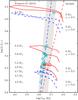 |
Fig. 6 Cepheid with masses determined by Evans et al. (2013) plotted as cyan open circles onto the blue loop portions of evolutionary tracks. Rotating tracks are drawn as solid red, non-rotating ones as dashed blue lines, the IS as in Fig. 2. |
Few model-independent Cepheid masses are known in the literature, and unfortunately, their associated uncertainties are rather large. In Fig. 7, we compare the model-independent masses shown in Evans et al. (2011) with the M − L relations presented in Fig. 5 above. This comparison is not very conclusive, unfortunately, though it does seem to favor the rotating M − L region shown. An interesting test to perform would be to investigate the Cepheid SU Cyg in terms of its observables related to rotation, since its location in the diagram is only consistent with virtually no rotation. Note that M − L relations are sensitive to metallicity in the sense that lower metallicity models yield higher luminosity. This is important to keep in mind when considering the LMC Cepheid OGLE-LMC-CEP-0227 (Pietrzyński et al. 2010) shown by green error bars.
While there does exist a degeneracy between the adopted value for the overshooting parameter and the rotation rate in terms of the M − L relation, rotation has implications on a star’s evolution that may be observable in the late stages of its evolution. For instance, rotation leads to enhanced helium surface abundance and modified CNO element abundance ratios, see Sect. 3.5. For Cepheids of a fixed mass, enhanced helium abundance would increase pulsation amplitudes, since the total amount of helium in the partial ionization zone would be increased, see Sect. 3.5.1. Furthermore, rotating models predict surface velocities that are clearly within the detectable range, cf. Sect. 3.3. Hence, the present rotating models make several potentially observable predictions that can be used to constrain the value of ω for a given Cepheid, and help to distinguish between evolutionary effects due to rotation and those due to higher core overshooting.
To summarize the above, the current mass discrepancy (on the order of 10−20%) can be explained by a combination of increased luminosity due to rotation and luminosity differences between Cepheids on second and third IS crossings.
 |
Fig. 7 Observed (non model-dependent) Cepheid masses (see Evans et al. 2011, and references therein) shown together with the M − L relations of Fig. 5. Luminosities were estimated by Evans et al. (2013) or Evans et al. (2011, Polaris & FF Aql) using the period−luminosity relationship by Benedict et al. (2007). The green error bars labeled “Cep227” show the highly accurate mass estimate for OGLE-CEP-LMC-0227 (Pietrzyński et al. 2010), where the luminosity was calculated from the published radius and temperature. |
3.3. Surface gravity, radii, and equatorial velocity
As can be seen in the D panels of Figs. 3 and 4, rotation impacts surface gravity, log g, during the IS crossings. Qualitatively similar in behavior to the increase in luminosity due to rotation, rotating models tend to have lower log g, and the range of log g values between the two crossings increases with rotation. This is no surprise, since log g and L are intimately linked via the M − L relationship. Since log g is related to stellar radius, rotation also impacts a Cepheid’s radius. These effects are particularly interesting to mention here, since log g and radius can be determined observationally and independently, providing constraints on a Cepheid’s crossing number and on ω.
Due to the conservation of angular momentum, stars with greater rotation rates on the MS can be expected to have greater rotational velocities also during the red (super-)giant phase. Panels E of Figs. 3 and 4 show the dependence of the equatorial surface velocity for the 7 M⊙ models, veq, on initial rotation rate during the second and third crossings: veq increases during the second crossing, and decreases during the third. The minimum and maximum values during the entire blue loop are indicated by up- and downward facing triangles, respectively.
Range of equatorial velocities veq in km s-1 predicted by models with ω = 0.5 for three different masses upon entering and exiting the blue (BE) and red (RE) edges of the IS.
Equatorial velocities predicted for models with ω = 0.5 for 5, 7, and 9 M⊙ models between the red (RE) and blue (BE) edges of the IS are listed in Table 2. veq tends to be consistently larger on the second crossing than on the third due to larger radius (lower log g). Given the predictions in Table 2, the presence of high vsini would tend to be indicative of a Cepheid being on the second crossing.
At the velocities predicted here, rotation should be readily observed by spectral line broadening. A first estimate of the average veq based on a sample of 97 classical Cepheids observed with the high-resolution spectrograph Coralie as part of an observing program to search for Cepheids associated with open clusters (Anderson et al. 2013) yields ⟨ veq ⟩ ≈ 12.3 km s-1 (Anderson 2013). A detailed comparison with observed surface velocities is currently in preparation. Three published observational studies found veq ≲ 10 km s-1 (Bersier & Burki 1996, using CORAVEL), vsini ≤ 16 km s-1 (Nardetto et al. 2006, estimates of vsini in their Table 2), and 4.9 ≤ vsini ≤ 17.7 km s-1 (De Medeiros et al. 2014, Cepheids identified via cross-match with the Variable Star Index, cf. Watson 2006).
At first sight, this comparison may appear to indicate overestimated predictions for veq for models with initial ω = 0.5. Note, however, that the predicted values of veq vary significantly between the different crossings, within each crossing, as a function of mass (or period), and are moreover strongly dependent on the choice of instability strip (bluer boundary = more contracted = higher veq). A detailed comparison must therefore take into account the crossings, temperature, masses (periods), and be based on a sufficiently large sample in order to deal with the randomly oriented rotation axes.
3.4. Cepheid ages and lifetimes
Rotating models yield older Cepheids than non-rotating ones (see panels F in Figs. 3 and 4), since rotation increases the MS lifetime of stars. For example, the difference in mean age during the second crossing between the non-rotating 7 M⊙ model (49.4 Myr), and the ω = 0.5 model of the same mass (58.6 Myr) is approximately 20%. Additional ages for Cepheid models of 5, 7, and 9 M⊙ models for different initial rotation rates are listed in Table 3. It is evident from the table that moderate rotation (ω = 0.5) causes a systematic increase in log a of approximately 0.08 dex, regardless of mass. Hence, the present models suggest that (rotating) real Cepheids may be systematically older by 20% than predicted by non-rotating models. Such considerations are relevant for calibrations of period−age relations (Bono et al. 2005) and their applications for constraining star formation histories, e.g. of the Galactic nuclear bulge (Matsunaga et al. 2011).
Cepheid ages for three different masses and rotation rates.
Predicted timescales relevant for Cepheids of different initial mass and rotation rate.
Besides age, rotation also impacts the duration of blue loops, and therefore Cepheid lifetimes (the time spent crossing the IS). Cepheid lifetimes and blue loop durations are listed in kyr in Table 4 covering three rotation rates with three initial masses for both the Bono et al. (2000b) and Tammann et al. (2003) instability strips. We note here that the 5 M⊙ models are affected by helium spikes during the third crossing. These occasional sudden increases of available helium can extend the lifetime of the third crossing significantly, if they occur inside the IS. However, Cepheid lifetime estimates depend much more strongly on the definition used for the IS boundaries than on these He spikes. Hence, the reader is advised to consider the following discussion merely as an indicator of tendencies.
The overall trends predicted for Cepheid lifetimes in Table 4 are as follows:
-
Lifetime estimates for the 5 and 7 M⊙ models are much longer (by a factor 2–3 in the case of 5 M⊙) when adopting the Tammann et al. (2003) IS rather than the Bono et al. (2000b) IS. The longer lifetimes can be explained by the greater width (in Teff) of the former IS definition and its bluer hot edge (evolution slower on the blue edge than the red). For 9 M⊙ models, the Bono et al. (2000b) IS predicts longer lifetimes due to its wedge shape.
-
First crossings are much faster than second or third crossings. The first crossing lifetime increases towards lower masses.
-
The larger the mass, the longer the time spent on the first crossing, relative to the second or third. Hence, the larger the mass, the more probable it is for a Cepheid to be observed during the first crossing.
-
Cepheid lifetimes for the 5 M⊙ model are by far the longest. Compared to 7 M⊙ models, 5 M⊙ models predict lifetimes that are at least an order of magnitude longer, depending strongly on the IS boundaries adopted and on rotation. The reason is that evolution along the blue loop is slowest at the tip of the blue loop, which lies square inside the IS for these models.
-
For the 5 M⊙ model, the third crossing is always slower than the second. However, this is not always the case for the higher-mass models.
-
The fractional time spent inside the IS, τCep,total/τloop, decreases with increasing mass. This is related to the speed at which a star evolves along the IS. As a result, a 5 M⊙ red giant is more likely to be caught (observed) during the Cepheid stage than an ordinary red giant of 7 or 9 M⊙. This is in addition to the effect of the IMF.
-
The total lifetimes of intermediate and high mass Cepheids depend less on rotation than low-mass Cepheids do.
Better resolution in rotation rate regarding Cepheid lifetimes is provided for the 7 M⊙ model in panels G of Figs. 3 and 4, though no clear trend is discernible.
3.5. Surface abundance enrichment
Rotational mixing creates effects that can impact Cepheid surface abundances during two different evolutionary stages. First, during the MS, rotational shear creates turbulence that slowly mixes material processed in the core throughout the radiative envelope, leading to enhanced surface abundances of helium and of nitrogen relative to carbon and oxygen. When the star evolves to become a red giant or supergiant, the core material is carried to the stellar surface during the first dredge-up phase when the star develops a deep convective envelope during its approach of the Hayashi track after the first IS crossing. Hence, two kinds of surface abundance enhancement have to be distinguished: the rotational enhancement occurring towards the end of the main sequence, and the dredge-up related enhancement. As the predictions presented in the following clearly show, both kinds of surface abundance enhancement depend on mass and rotation.
Abundance enhancement of element Xi is defined as the
post-dredge-up (index Cep) increase in mass fraction relative to the initial value (on the
ZAMS, index 0), i.e.,  (7)ΔXi has two
contributions, one due to the dredge-up (index DU), and one related to rotational
enhancement on the MS (index MS).
(7)ΔXi has two
contributions, one due to the dredge-up (index DU), and one related to rotational
enhancement on the MS (index MS).
For CNO elements, we express the abundance enhancement in logarithmic units relative to
hydrogen, where, in the case of nitrogen (N):
![Mathematical equation: \begin{eqnarray} {\rm [N/H]} = \log{\left(\frac{X_{\rm N,Cep}}{{A}_{{\rm N}} \cdot X_{\rm H,Cep} } \right) } - \log{ \left( \frac{{\it X}_{\rm N,\odot}}{{\it A}_{{\rm N}} \cdot {\it X}_{{\rm H,\odot}} } \right) } \equiv \Delta {\rm [N/H]}. \end{eqnarray}](/articles/aa/full_html/2014/04/aa22988-13/aa22988-13-eq101.png) (8)Here, AN denotes the
atomic mass number of nitrogen. Similarly, for ratio of nitrogen to carbon,
(8)Here, AN denotes the
atomic mass number of nitrogen. Similarly, for ratio of nitrogen to carbon,
![Mathematical equation: \begin{eqnarray} \Delta \rm{[N/C]} \equiv \rm{[N/C]} \equiv \rm{[N/H]} - \rm{[C/H]}. \end{eqnarray}](/articles/aa/full_html/2014/04/aa22988-13/aa22988-13-eq103.png) (9)Figure 8
shows predicted surface abundance enhancements for helium, ΔYS, as well as
N relative to C and N relative to O as a function of initial rotation rate for
7
M⊙ models. Similarly, Figs. 9–11 show the same
information as functions of both rotation (gray scaled, where darker represents higher
ω) and
mass. In all these figures, terminal age main sequence (TAMS) values are indicated as
upward facing triangles. Post dredge-up values are shown as circles. As per their
definition, initial (ZAMS) values are 0.
(9)Figure 8
shows predicted surface abundance enhancements for helium, ΔYS, as well as
N relative to C and N relative to O as a function of initial rotation rate for
7
M⊙ models. Similarly, Figs. 9–11 show the same
information as functions of both rotation (gray scaled, where darker represents higher
ω) and
mass. In all these figures, terminal age main sequence (TAMS) values are indicated as
upward facing triangles. Post dredge-up values are shown as circles. As per their
definition, initial (ZAMS) values are 0.
 |
Fig. 8 Surface abundance enrichment for the 7 M⊙ model as a function of initial rotation. Top panel shows surface helium mass fraction relative to starting value, center and bottom panels show [N/C] and [N/O] enhancement relative to starting (solar) value. Quantities before first dredge-up are shown as upward triangles, post-dredge-up as circles. |
Since rotational mixing can enhance surface abundances towards the TAMS, the presence of enriched abundances is not an unambiguous argument for excluding a Cepheid’s crossing the IS for the first time. As shown in the following subsections, the TAMS enhancement depends primarily on rotation, but also on mass. Thus, especially high mass, i.e., long-period, Cepheids are expected to exhibit enhanced abundances even if they are on the first crossing. However, an absence of enhanced abundances may be indicative of small ω (rotational history of the Cepheid) and a first IS crossing.
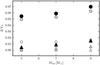 |
Fig. 9 Helium surface mass fraction enhancement as a function of mass and initial rotation. Open symbols represent non-rotating models, solid gray symbols ω = 0.5, and solid black symbols ω = 0.8. Pre-dredge-up enhancement is drawn as triangles, post-dredge-up values as circles. |
3.5.1. Helium
Figure 9 clearly shows that even small amounts of rotation considerably increase the post-dredge-up helium surface mass fraction YS drawn as circles whose grayscale represents rotation rate (the darker, the faster). High rotation rates (ω> 0.5) are required to cause significant enrichment on the MS (TAMS predictions drawn as upward triangles with same grayscale), although enhancement during the MS is a factor of 5–6 smaller than the post-dredge-up enhancement.
For a fixed mass, an increase in YS due to rotation also signifies an increase in the total mass of helium in the He partial ionization zone, ΔMHe. This should affect the pulsations, since the amplitude of light variation may depend on He abundance. For instance, Kovtyukh (1998) predicted an increase in amplitude (δL ∝ ΔMHe/P), where P denotes pulsation period. According to Cogan et al. (1980), an increase of He mass fraction by 0.1 would increase the light amplitude by 0.25 mag, and radial velocity amplitude by 15 m s-1. However, in a recent investigation using nonlinear convective hydrodynamical models, Marconi et al. (2013) found only a weak dependence of pulsation amplitude to He abundance in the range of YS = 0.26,0.27,0.28 (note that the predicted enhancement, ΔYS, due to rotation can reach up to 0.05, cf. Fig. 8). Furthermore, pulsation amplitudes might be expected to decrease with increased YS due to lowered opacity in the partial ionization zone (G. Bono, priv. comm.). In conclusion, pulsation amplitudes probably depend (in one way or another) on YS, which is affected by rotation. Hence, the observed spread in observed photometric and velocimetric amplitudes (e.g. Bono et al. 2000b) may partly be due to variations in rotation rate. However, the present static models cannot by themselves predict the behavior of pulsations.
3.5.2. CNO elements
In the intermediate-mass stars considered here, H-burning is dominated by the CNO cycle. Besides producing helium from hydrogen, the CNO cycle gradually transforms C and O into 14N, since this element has the slowest rate of destruction (Maeder 1985). Hence, the ratios [N/C] and [N/O] are expected to be modified by rotation. We show the behavior of Δ [N/C] and Δ [N/O] as a function of rotation rate in the two lower panels of Fig. 8.
The TAMS enhancement is predicted to be much more noticeable for CNO elements than for helium, due to the fact that very early during the core H-burning phase, strong gradients of CNO elements appear between the convective core and the envelope, triggering fast diffusion timescales. Clearly, the MS enhancement of nitrogen depends primarily on rotation, as seen by the upward-facing triangles in Figs. 10 and 11 that are grayscaled for rotation rates (faster is darker). For fast rotating models of sufficiently high mass (>7 M⊙) the rotational mixing during the MS leads to stronger abundance enhancement than dredge-up in non-rotating models of the same mass. It furthermore appears that the contribution of dredge-up to enhanced abundances is rather insensitive to rotation, though the MS enhancement is very sensitive to rotation. This is an interesting contrast with helium abundance enhancement, pointing out the large difference between the He and CNO abundance gradients between the convective core and the radiative envelope. In summary, the modification of CNO abundances due to rotational mixing during the MS and due to dredge-up are of similar orders, with the rotational effect dominating for the highest-mass models. In contrast, helium enhancement occurs primarily during dredge-up.
We mention here that puzzling CNO abundance predictions made by rotating Geneva models of blue supergiant stars were previously pointed out by Saio et al. (2013). Although a detailed comparison with observed abundance enhancement will be presented in a publication to follow soon, we can already mention that the enhancement of CNO elements predicted by the present models appears systematically too high by up to 0.2 dex. However, measuring CNO abundances in the extended atmospheres of Cepheids is sufficiently complex to leave room for significant systematic errors associated with the measurement.
3.6. Tracing Cepheid evolution via period changes
Cepheids are among the rare objects whose evolution can be observed on human timescales
thanks to variations in period that are interpreted as being due to contraction (period
becomes shorter) or expansion (longer) as the Cepheid evolves along the IS crossing. The
underlying idea is that in a radially pulsating star the pulsation period, P, is intimately linked
with the mean density in solar units,  ,
via the relation
,
via the relation  (10)This relation was first investigated in the
context of stellar pulsations by Ritter (1879).
Equation (10) was first applied to
investigate the rate of progress of stellar evolution by Eddington (1918, 1919), demonstrating
that the main energy source of stars could not be contraction. Thus, rates of period
change have provided and continue to provide crucial tests of stellar evolution.
(10)This relation was first investigated in the
context of stellar pulsations by Ritter (1879).
Equation (10) was first applied to
investigate the rate of progress of stellar evolution by Eddington (1918, 1919), demonstrating
that the main energy source of stars could not be contraction. Thus, rates of period
change have provided and continue to provide crucial tests of stellar evolution.
Estimates for predicted rates of period change can be obtained from evolutionary tracks
such as the present ones, since variations in mean density are time resolved during the IS
crossings. Starting from the time derivative of the period−density relation (Eq. (10)), we obtain  (11)
(11) (12)Adopting the period-dependence of
Q as
investigated by Saio & Gautschy (1998), i.e.,
(12)Adopting the period-dependence of
Q as
investigated by Saio & Gautschy (1998), i.e.,
![Mathematical equation: \begin{eqnarray} Q = 3.47 \times 10^{-2} + 5.2 \times 10^{-3} \log{P} + 2.8 \times 10^{-3} \,[\log{P}]^{2}, \label{eq:pulsationconstant} \end{eqnarray}](/articles/aa/full_html/2014/04/aa22988-13/aa22988-13-eq127.png) (13)with 0.035 ≤ Q ≤ 0.050, we can
estimate the importance of the first term in Eq. (12) using the average densities predicted by the models. We find this term to be
close to unity and thus negligible for a first order estimate. A more detailed
investigation would, however, involve a consistent determination of pulsation periods for
these models. With
(13)with 0.035 ≤ Q ≤ 0.050, we can
estimate the importance of the first term in Eq. (12) using the average densities predicted by the models. We find this term to be
close to unity and thus negligible for a first order estimate. A more detailed
investigation would, however, involve a consistent determination of pulsation periods for
these models. With  and dividing by P, we obtain a simple way
to predict rates of period change to first order from the evolutionary tracks via
and dividing by P, we obtain a simple way
to predict rates of period change to first order from the evolutionary tracks via
 (14)Figure 12 shows the range of |
Ṗ | /P estimated using Eq. (14) as a function of ω for second and third
crossings. The absolute value is plotted here in order to have the direct comparison of
the rates of period change for both crossings.
(14)Figure 12 shows the range of |
Ṗ | /P estimated using Eq. (14) as a function of ω for second and third
crossings. The absolute value is plotted here in order to have the direct comparison of
the rates of period change for both crossings.
 |
Fig. 12 Absolute values of predicted rates of period change for several Cepheid models are shown against initial rotation rate ω. Predictions for the Bono et al. (2000b) IS are drawn as black, blue, and red vertical lines for the 5, 7 and 9 M⊙ models, respectively. Gray shaded bars represent the predictions assuming the Tammann et al. (2003) IS. Second crossing Cepheids are offset to slightly lower ω, third crossing Cepheids to higher ω for visibility. Period decreases along the second crossing, and increases along the third. Per-mass averages are shown as annotated horizontal dotted lines. |
As expected from Cepheid lifetimes, higher mass stars are predicted to show faster rates
of period change. No obvious dependence on ω emerges, although the values predicted for
Ṗ/P do exhibit some fluctuations.
The only slight tendency seen is that 7
M⊙ models tend to show increasing
 with increasing ω on the second crossing,
whereas the opposite is true on the third crossing. Furthermore, the ranges of
Ṗ/P covered in a given crossing
depend quite strongly on the IS boundaries adopted.
with increasing ω on the second crossing,
whereas the opposite is true on the third crossing. Furthermore, the ranges of
Ṗ/P covered in a given crossing
depend quite strongly on the IS boundaries adopted.
Period changes can be measured observationally using O−C diagrams, and are typically given in terms of the quantity Ṗ/P. In the Galaxy, observational rates of period change have been determined for nearly 200 Cepheids (Turner et al. 2006), providing good statistics and long baselines that make this an exciting tool for comparisons with stellar models. Comparing the rates of period change predicted by the present models with the observed rates Turner et al. (2006, Fig. 3) yields very good agreement.
Several effects not considered here are likely to impact the predicted rates of period change, including for instance the distribution of helium inside the envelope, or the dependence of the neglected first term in Eq. (12) on density (which depends on ω). However, consistent determinations of the IS location and pulsation periods are out of scope for this paper. These and a detailed comparison with observed rates of period change are therefore postponed to a future publication.
3.7. Intrinsic dispersion of the Cepheid PLR
As was shown in the previous sections, rotation together with the crossing number lifts the uniqueness of the mass−luminosity relationship for Cepheids and affects their densities. One of the cornerstones of the universal distance scale is the empirically-calibrated period−luminosity relation (PLR, Leavitt 1908; Leavitt & Pickering 1912) that attributes luminosities (or absolute magnitudes) to values of the pulsation period alone (e.g. Benedict et al. 2007; Freedman et al. 2012), or to period and color (e.g. Tammann et al. 2003; Sandage et al. 2004, leading to period−luminosity−color relations). PLR calibrations are performed on real stellar populations (or at least samples of stars), whose constituents formed following an ω-distribution. The prediction that a Cepheid’s luminosity depends on ω leads to the question how this may affect the PLR.
Figure 13 shows the relation between the
(logarithmic) luminosity and the logarithm of the inverse average density
( , cf. Eq. (10)) for the 5,
7, and 9
M⊙ models with (ω = 0.5) and without
rotation. Second and third crossings are distinguished by line style (solid/dashed).
, cf. Eq. (10)) for the 5,
7, and 9
M⊙ models with (ω = 0.5) and without
rotation. Second and third crossings are distinguished by line style (solid/dashed).
 |
Fig. 13 Cepheid luminosity versus log P/Q for 5, 7 and 9 M⊙ models in the second (solid lines) and third (dashed lines) crossings. Rotating models with ω = 0.5 are shown in black, non-rotating models in gray. At a given value of log P/Q, log L can easily vary by more than 0.1 dex (25%), depending on ω as well as the crossing number. Hence, rotation leads to an intrinsic dispersion of the period−luminosity relationship. |
It is clear from the figure that a range of luminosities is predicted for different ω values at a given log P/Q. Models on different crossings can have the same effect. Hence, the present models predict an intrinsic scatter in luminosity at fixed log P/Q that is due to luminosity differences among crossings and initial rotation rates, enabled by the finite width (in temperature) of the IS. Naturally, if the boundaries of the IS should depend on rotation, then this may also affect the intrinsic dispersion of the Cepheid PLR. Note that color or effective temperature may likely be used to distinguish between the various luminosities associated with a given value of log P/Q (e.g. Tammann et al. 2003).
From Fig. 13 it appears that the maximal difference in log L (at fixed log P/Q) due to rotation can be larger than the one due to confused crossing numbers. However, it should be remembered that luminosity is relatively stable over a range of ω for Cepheids of a given mass, cf. Figs. 3 and 4. Hence, the dispersion due to rotation alone is probably not very large, and the differences due to the increased luminosity on the third crossing (relative to the second crossing and at fixed log P/Q) should be the dominant source of dispersion in the PLR.
4. Discussion
4.1. Rotation vs. overshoot and the mass discrepancy
In Sect. 3.2 we investigate Cepheid masses inferred using rotating models and find that neglecting the effect of rotation and crossing number on luminosity can lead to errors in the order of magnitude of the mass discrepancy. Furthermore, the “average” M − L relationship of rotating models, i.e., neglecting the crossing number and using the average rotation rate ω = 0.5, is consistent with an M − L relation assuming significantly stronger overshooting. This degeneracy can be easily explained, since both rotation and overshoot increase core size and therefore produce higher luminosities for lower masses.
However, besides increased luminosity, core-overshooting makes few other predictions, acting essentially like a fudge factor that is increased until evolutionary masses match pulsational ones. On the other hand, rotation is observed in most stars, and especially so in the progenitors of Cepheids. Furthermore, rotation makes several testable predictions of observable quantities. Accordingly, a detailed comparison of the predictions presented here with observational quantities is currently in preparation.
Another possibilty of diminishing the mass discrepancy, i.e., lowering the evolutionary mass at fixed luminosity, is to include pulsation-enhanced mass-loss (e.g. Neilson & Lester 2008; Neilson et al. 2011). This mechanism is not currently included in our models, and its total predicted mass loss depends strongly on Cepheid lifetimes, i.e., on the position and width of the IS. Observational constraints such as those by Matthews et al. (2012) are crucial to further investigate this issue.
4.2. Dependence on IS boundary definition
Clearly, adopting a given set of IS boundaries impacts the predictions obtained from our static evolutionary models, yielding IS boundary-dependent predictions for the range of luminosities, surface gravities, equatorial velocities, etc. This problem, however, is common in Cepheid research, complicated by model assumptions in the case of theoretical boundaries and by the correction for reddening and extinction in observational studies. In order to be sensitive to such systematic differences for the predicted values, two different IS boundary definitions were employed, one theoretically (Bono et al. 2000b) and one empirically derived (Tammann et al. 2003).
The predictions obtained from the two different IS boundary definitions do generally vary quite a bit, although not by an order of magnitude. Generally speaking, the Tammann et al. (2003) IS is bluer, i.e., hotter, and therefore predicts more luminous Cepheids with higher surface gravity and surface rotation. As a result, the “average” M − L relation for the Tammann et al. (2003) IS predicts even lower mass at a given luminosity than the (Bono et al. 2000b) IS, although the difference is generally <1%. As seen in Fig. 12, predicted rates of period change may also depend on the IS boundaries adopted. Other predicted quantities such as surface abundance enrichment, or Cepheid ages do not significantly depend on the IS definition.
For a given position in the HRD, rotation lowers stellar mean density hydrostatically, decreasing the temperature gradient. Thus, rotation is likely to affect the location of the IS boundaries in the HRD, since pulsational instability depends on the location of the partial He-ionization zone inside a star’s envelope as well as the total mass of helium in that region. An ω-dependence of IS boundaries would require to replace the canonical notion of a single sharply defined IS with a transition zone spanned by instability trips corresponding to different ω, with implications for the question of purity of the IS. Such questions shall be addressed in a future study focusing on the pulsational instability of the present models.
5. Conclusions
This paper presents the first detailed investigation of the effect of rotation on evolutionary models of classical Cepheids. The study is based on the latest state-of-the-art rotating Geneva models (cf. E12) that incorporate a homogeneous and self-consistent treatment of rotation over the entire evolutionary cycle for a wide range of stellar masses. A dense grid of evolutionary tracks of different rotation rates for intermediate-mass stars is available from G13 and enables a detailed investigation not only as a function of initial rotation rate, ω, but also as a function of time during the IS crossings.
Qualitative predictions are made as a function of initial rotation rate for an array of observable quantities, such as surface gravities, surface abundance enhancement, surface velocities, radii, and rates of period change. These will be quantified and compared to observational constraints in a subsequent publication.
The key results of this investigation are:
-
1.
M − L relations depend on ω. This is true for all stars during all stages of evolution, although the difference is more obvious during the blue loop phase.
-
2.
For Cepheids, an M − L relation at fixed ω furthermore depends on crossing number. The greater ω, the greater the difference between the crossings, since rotation broadens the blue loops.
-
3.
The Cepheid mass discrepancy problem vanishes when rotation and crossing number are taken into account, without a need for high core overshooting values or enhanced mass loss.
-
4.
Differences in initial rotation rate and crossing number between Cepheids of identical mass and metallicity create intrinsic scatter around the average values predicted. This is true for most parameters considered here, among them in particular the Cepheid period−luminosity relation, i.e., rotation is a source of intrinsic dispersion for the PLR.
-
5.
Rotational mixing can significantly enhance surface abundances during the MS phase. Consequently, enriched surface abundances do not unambiguously distinguish Cepheids on the first crossing from ones on second or third crossings.
-
6.
Rotating models predict older Cepheids than currently assumed due to longer MS lifetimes.
Arguably the two most important results are result numbers 3 and 4, i.e., the solution of the mass discrepancy problem and the prediction of intrinsic scatter for Cepheid observables at fixed mass and metallicity. Since the mass discrepancy has been claimed to be solved by several other studies in the past, one may be reluctant to immediately adopt rotation as the best explanation. However, result 4 may provide the smoking gun for distinguishing between rotation and other effects such as core overshooting. While it would be difficult to explain why stars of identical mass and metallicity should present different overshooting values (leading to the observed scatter in, say, radius or luminosity), dispersion arises naturally when a dispersion in initial velocity is considered, which is an observational fact.
As this paper shows, the effects of rotation on Cepheid populations are highly significant, ranging from issues related to inferred masses to the prediction of systematic effects relevant for the distance scale. Further related research is currently in progress.
Here, we employ l/HP = 1.6, which reproduces the positions of both red giant branch and the red supergiant stars, see Fig. 2 in E12.
Rotating models calculated here as in E12, where rotation is parametrized as v/vcrit, with vcrit denoting critical rotation. v/vcrit = 0.4 is equivalent to ω = 0.568.
Acknowledgments
The authors would like to acknowledge Nancy Remage Evans for her communication regarding model-independent mass-estimates of classical Cepheids and the referee, Giuseppe Bono, for his valuable comments. This research has made use of NASA’s Astrophysics Data System. C.G. acknowledges support from the European Research Council under the European Union’s Seventh Framework Programme (FP/2007-2013)/ERC Grant Agreement no 306901.
References
- Anderson, R. I. 2013, Ph.D. Thesis, University of Geneva, Switzerland [Google Scholar]
- Anderson, R. I., Eyer, L., & Mowlavi, N. 2013, MNRAS, 434, 2238 [NASA ADS] [CrossRef] [Google Scholar]
- Asplund, M., Grevesse, N., & Sauval, A. J. 2005, in Cosmic Abundances as Records of Stellar Evolution and Nucleosynthesis, eds. T. G. Barnes, III, & F. N. Bash, ASP Conf. Ser., 336, 25 [Google Scholar]
- Benedict, G. F., McArthur, B. E., Feast, M. W., et al. 2007, AJ, 133, 1810 [NASA ADS] [CrossRef] [Google Scholar]
- Bersier, D., & Burki, G. 1996, A&A, 306, 417 [Google Scholar]
- Bertelli, G., Girardi, L., Marigo, P., & Nasi, E. 2008, A&A, 484, 815 [NASA ADS] [CrossRef] [EDP Sciences] [Google Scholar]
- Bono, G., Caputo, F., Cassisi, S., et al. 2000a, ApJ, 543, 955 [NASA ADS] [CrossRef] [Google Scholar]
- Bono, G., Castellani, V., & Marconi, M. 2000b, ApJ, 529, 293 [NASA ADS] [CrossRef] [Google Scholar]
- Bono, G., Marconi, M., Cassisi, S., et al. 2005, ApJ, 621, 966 [NASA ADS] [CrossRef] [Google Scholar]
- Bono, G., Caputo, F., & Castellani, V. 2006, Mem. Soc. Astron. Italiana, 77, 207 [Google Scholar]
- Bono, G., Inno, L., Matsunaga, N., et al. 2013, in IAU Symp. 289, ed. R. de Grijs, 116 [Google Scholar]
- Caputo, F., Bono, G., Fiorentino, G., Marconi, M., & Musella, I. 2005, ApJ, 629, 1021 [NASA ADS] [CrossRef] [Google Scholar]
- Cassisi, S., & Salaris, M. 2011, ApJ, 728, L43 [NASA ADS] [CrossRef] [Google Scholar]
- Castellani, V., Chieffi, A., & Straniero, O. 1992, ApJS, 78, 517 [NASA ADS] [CrossRef] [Google Scholar]
- Christy, R. F. 1968, QJRAS, 9, 13 [NASA ADS] [Google Scholar]
- Cogan, B. C., Cox, A. N., & King, D. S. 1980, Space Sci. Rev., 27, 419 [NASA ADS] [CrossRef] [Google Scholar]
- Cox, A. N. 1980, ARA&A, 18, 15 [NASA ADS] [CrossRef] [Google Scholar]
- Crowther, P. A. 2001, in The Influence of Binaries on Stellar Population Studies, ed. D. Vanbeveren, Astrophys. Space Sci. Lib., 264, 215 [Google Scholar]
- de Jager, C., Nieuwenhuijzen, H., & van der Hucht, K. A. 1988, A&AS, 72, 259 [NASA ADS] [Google Scholar]
- De Medeiros, J. R., Alves, S., Udry, S., et al. 2014, A&A, 561, A126 [NASA ADS] [CrossRef] [EDP Sciences] [Google Scholar]
- Eddington, A. S. 1918, The Observatory, 41, 379 [NASA ADS] [Google Scholar]
- Eddington, A. S. 1919, The Observatory, 42, 338 [NASA ADS] [Google Scholar]
- Ekström, S., Georgy, C., Eggenberger, P., et al. 2012, A&A, 537, A146 (E12) [NASA ADS] [CrossRef] [EDP Sciences] [Google Scholar]
- Evans, N. R., Berdnikov, L., Gorynya, N., Rastorguev, A., & Eaton, J. 2011, AJ, 142, 87 [NASA ADS] [CrossRef] [Google Scholar]
- Evans, N. R., Bond, H. E., Schaefer, G. H., et al. 2013, AJ, 146, 93 [NASA ADS] [CrossRef] [Google Scholar]
- Freedman, W. L., Madore, B. F., Scowcroft, V., et al. 2012, ApJ, 758, 24 [NASA ADS] [CrossRef] [Google Scholar]
- Georgy, C., Ekström, S., Granada, A., et al. 2013, A&A, 553, A24 (G13) [NASA ADS] [CrossRef] [EDP Sciences] [Google Scholar]
- Huang, W., Gies, D. R., & McSwain, M. V. 2010, ApJ, 722, 605 [NASA ADS] [CrossRef] [Google Scholar]
- Iglesias, C. A., & Rogers, F. J. 1991, ApJ, 371, 408 [NASA ADS] [CrossRef] [Google Scholar]
- Iglesias, C. A., & Rogers, F. J. 1996, ApJ, 464, 943 [NASA ADS] [CrossRef] [Google Scholar]
- Keller, S. C. 2008, ApJ, 677, 483 [NASA ADS] [CrossRef] [Google Scholar]
- Kippenhahn, R., & Weigert, A. 1994, Stellar Structure and Evolution, XVI (Astron. Astrophys. Lib. and Springer) [Google Scholar]
- Kovtyukh, V. V. 1998, Astron. Astrophys. Trans., 17, 15 [NASA ADS] [CrossRef] [Google Scholar]
- Lagarde, N., Decressin, T., Charbonnel, C., et al. 2012, A&A, 543, A108 [NASA ADS] [CrossRef] [EDP Sciences] [Google Scholar]
- Leavitt, H. S. 1908, Annals of Harvard College Observatory, 60, 87 [Google Scholar]
- Leavitt, H. S., & Pickering, E. C. 1912, Harvard College Observatory Circular, 173, 1 [Google Scholar]
- Maeder, A. 1985, in European Southern Observatory Conference and Workshop Proc., eds. I. J. Danziger, F. Matteucci, & K. Kjar, 21, 187 [Google Scholar]
- Maeder, A. 1997, A&A, 321, 134 [NASA ADS] [Google Scholar]
- Maeder, A. 2009, Physics, Formation and Evolution of Rotating Stars (Astronomy and Astrophysics Library and Springer) [Google Scholar]
- Maeder, A., & Meynet, G. 2000, ARA&A, 38, 143 [NASA ADS] [CrossRef] [Google Scholar]
- Maeder, A., & Meynet, G. 2001, A&A, 373, 555 [NASA ADS] [CrossRef] [EDP Sciences] [Google Scholar]
- Maeder, A., & Zahn, J.-P. 1998, A&A, 334, 1000 [NASA ADS] [Google Scholar]
- Marconi, M., Molinaro, R., Bono, G., et al. 2013, ApJ, 768, L6 [NASA ADS] [CrossRef] [Google Scholar]
- Matsunaga, N., Kawadu, T., Nishiyama, S., et al. 2011, Nature, 477, 188 [NASA ADS] [CrossRef] [PubMed] [Google Scholar]
- Matthews, L. D., Marengo, M., Evans, N. R., & Bono, G. 2012, ApJ, 744, 53 [NASA ADS] [CrossRef] [Google Scholar]
- Moskalik, P., Buchler, J. R., & Marom, A. 1992, ApJ, 385, 685 [NASA ADS] [CrossRef] [Google Scholar]
- Nardetto, N., Mourard, D., Kervella, P., et al. 2006, A&A, 453, 309 [NASA ADS] [CrossRef] [EDP Sciences] [Google Scholar]
- Neilson, H. R., & Lester, J. B. 2008, ApJ, 684, 569 [NASA ADS] [CrossRef] [Google Scholar]
- Neilson, H. R., Cantiello, M., & Langer, N. 2011, A&A, 529, L9 [NASA ADS] [CrossRef] [EDP Sciences] [Google Scholar]
- Pietrzyński, G., Thompson, I. B., Gieren, W., et al. 2010, Nature, 468, 542 [NASA ADS] [CrossRef] [PubMed] [Google Scholar]
- Pra da Moroni, P. G., Gennaro, M., Bono, G., et al. 2012, ApJ, 749, 108 [NASA ADS] [CrossRef] [Google Scholar]
- Reimers, D. 1975, Mem. Soc. Roy. Sci. Liège, 8, 369 [Google Scholar]
- Reimers, D. 1977, A&A, 61, 217 [NASA ADS] [Google Scholar]
- Ritter, A. 1879, Wiedemanns Annalen, 173 [Google Scholar]
- Saio, H., & Gautschy, A. 1998, ApJ, 498, 360 [NASA ADS] [CrossRef] [Google Scholar]
- Saio, H., Georgy, C., & Meynet, G. 2013, MNRAS, 433, 1246 [NASA ADS] [CrossRef] [Google Scholar]
- Sandage, A., Tammann, G. A., & Reindl, B. 2004, A&A, 424, 43 [NASA ADS] [CrossRef] [EDP Sciences] [Google Scholar]
- Seaton, M. J., Yan, Y., Mihalas, D., & Pradhan, A. K. 1994, MNRAS, 266, 805 [NASA ADS] [CrossRef] [Google Scholar]
- Slettebak, A. 1949, ApJ, 110, 498 [NASA ADS] [CrossRef] [Google Scholar]
- Stobie, R. S. 1969a, MNRAS, 144, 461 [NASA ADS] [Google Scholar]
- Stobie, R. S. 1969b, MNRAS, 144, 485 [NASA ADS] [Google Scholar]
- Stobie, R. S. 1969c, MNRAS, 144, 511 [NASA ADS] [Google Scholar]
- Tammann, G. A., Sandage, A., & Reindl, B. 2003, A&A, 404, 423 [NASA ADS] [CrossRef] [EDP Sciences] [Google Scholar]
- Turner, D. G. 2009, in AIP Conf. Ser., eds. J. A. Guzik, & P. A. Bradley, 59 [Google Scholar]
- Turner, D. G., Abdel-Sabour Abdel-Latif, M., & Berdnikov, L. N. 2006, PASP, 118, 410 [NASA ADS] [CrossRef] [Google Scholar]
- Vink, J. S., de Koter, A., & Lamers, H. J. G. L. M. 2001, A&A, 369, 574 [NASA ADS] [CrossRef] [EDP Sciences] [Google Scholar]
- Watson, C. L. 2006, Soc. Astron. Sci. Ann. Symp., 25, 47 [NASA ADS] [Google Scholar]
- Worthey, G., & Lee, H.-C. 2011, ApJS, 193, 1 [NASA ADS] [CrossRef] [EDP Sciences] [Google Scholar]
- Zahn, J.-P. 1992, A&A, 265, 115 [NASA ADS] [Google Scholar]
All Tables
Range of equatorial velocities veq in km s-1 predicted by models with ω = 0.5 for three different masses upon entering and exiting the blue (BE) and red (RE) edges of the IS.
Predicted timescales relevant for Cepheids of different initial mass and rotation rate.
All Figures
|
Fig. 1 Comparison of Geneva stellar evolutionary tracks (solid black lines: non-rotating; dotted black lines: v/vcrit = 0.4) with Padova tracks (Bertelli et al. 2008, solid cyan lines), and tracks by Castellani et al. (1992, solid red lines) and Lagarde et al. (2012, solid green lines = non-rotating; dotted green lines = v/vcrit = 0.3. The instability strips by Bono et al. (2000b, wedge-shaped dark blue solid lines) and Tammann et al. (2003, gray shaded area) are also included. |
| In the text | |
|
Fig. 2 Evolutionary tracks for 7 M⊙ solar-metallicity models with different initial rotation rates: ω = 0.0,0.5,0.8 are drawn as solid blue, dashed green and dash-dotted red lines, respectively. The red and blue edges of the instability strip (IS) according to Bono et al. (2000b) are indicated by dashed lines. Grid points inside the IS are marked as solid circles. The Tammann et al. (2003) IS is shown as a shaded gray area. |
| In the text | |
|
Fig. 3 Predictions for 7 M⊙ Cepheids on the second crossing as function of ω. Panels A) through G) show bolometric magnitude, luminosity, effective temperature, surface gravity, equatorial velocity, age, and lifetime. The range of values during the IS crossing is shown as black lines for the IS definition by Bono et al. (2000b), and as a light gray shade for the IS from Tammann et al. (2003). On the second crossing, all parameters increase during the evolution along the blue loop, except for τCep, which shows the duration of the IS crossing. Triangles in panel E) show the extreme values for surface velocity at the beginning of the blue loop near the Hayashi track (minimal) and at its greatest extension (maximal). |
| In the text | |
|
Fig. 4 Analogous to Fig. 3 for the third crossing. Note that the parameters in panels A) through E) are decreasing during the third IS crossing. |
| In the text | |
|
Fig. 5 Mass−luminosity relationship for rotating (ω = 0.5, cyan, consistently higher luminosity) and non-rotating Cepheids (yellow, lower luminosity). Shaded areas show the range of values between the second (squares) and third (circles) crossings. Solid symbols are based on grid models, open symbols indicate models obtained via the web-based interpolation tool. The dashed red line that crosses the non-rotating area represents the M − L relation by Caputo et al. (2005, their Eq. (2) with Z = 0.014, Y = 0.27 whose investigation was based on the models by Bono et al. (2000a) and does not account for convective core overshooting. The solid red line crossing through the area delineated by rotating models is the M − L relationship used by Evans et al. (2013), which assumes a value of dover/HP = 0.2 for convective core overshooting (based on models by Prada Moroni et al. 2012). |
| In the text | |
|
Fig. 6 Cepheid with masses determined by Evans et al. (2013) plotted as cyan open circles onto the blue loop portions of evolutionary tracks. Rotating tracks are drawn as solid red, non-rotating ones as dashed blue lines, the IS as in Fig. 2. |
| In the text | |
|
Fig. 7 Observed (non model-dependent) Cepheid masses (see Evans et al. 2011, and references therein) shown together with the M − L relations of Fig. 5. Luminosities were estimated by Evans et al. (2013) or Evans et al. (2011, Polaris & FF Aql) using the period−luminosity relationship by Benedict et al. (2007). The green error bars labeled “Cep227” show the highly accurate mass estimate for OGLE-CEP-LMC-0227 (Pietrzyński et al. 2010), where the luminosity was calculated from the published radius and temperature. |
| In the text | |
|
Fig. 8 Surface abundance enrichment for the 7 M⊙ model as a function of initial rotation. Top panel shows surface helium mass fraction relative to starting value, center and bottom panels show [N/C] and [N/O] enhancement relative to starting (solar) value. Quantities before first dredge-up are shown as upward triangles, post-dredge-up as circles. |
| In the text | |
|
Fig. 9 Helium surface mass fraction enhancement as a function of mass and initial rotation. Open symbols represent non-rotating models, solid gray symbols ω = 0.5, and solid black symbols ω = 0.8. Pre-dredge-up enhancement is drawn as triangles, post-dredge-up values as circles. |
| In the text | |
 |
Fig. 10 Analogous to Fig. 9 for [N/C] surface abundance enhancement. |
| In the text | |
 |
Fig. 11 Analogous to Fig. 9 for [N/O] surface abundance enhancement. |
| In the text | |
|
Fig. 12 Absolute values of predicted rates of period change for several Cepheid models are shown against initial rotation rate ω. Predictions for the Bono et al. (2000b) IS are drawn as black, blue, and red vertical lines for the 5, 7 and 9 M⊙ models, respectively. Gray shaded bars represent the predictions assuming the Tammann et al. (2003) IS. Second crossing Cepheids are offset to slightly lower ω, third crossing Cepheids to higher ω for visibility. Period decreases along the second crossing, and increases along the third. Per-mass averages are shown as annotated horizontal dotted lines. |
| In the text | |
|
Fig. 13 Cepheid luminosity versus log P/Q for 5, 7 and 9 M⊙ models in the second (solid lines) and third (dashed lines) crossings. Rotating models with ω = 0.5 are shown in black, non-rotating models in gray. At a given value of log P/Q, log L can easily vary by more than 0.1 dex (25%), depending on ω as well as the crossing number. Hence, rotation leads to an intrinsic dispersion of the period−luminosity relationship. |
| In the text | |
Current usage metrics show cumulative count of Article Views (full-text article views including HTML views, PDF and ePub downloads, according to the available data) and Abstracts Views on Vision4Press platform.
Data correspond to usage on the plateform after 2015. The current usage metrics is available 48-96 hours after online publication and is updated daily on week days.
Initial download of the metrics may take a while.