| Issue |
A&A
Volume 564, April 2014
|
|
|---|---|---|
| Article Number | A90 | |
| Number of page(s) | 14 | |
| Section | Stellar atmospheres | |
| DOI | https://doi.org/10.1051/0004-6361/201322881 | |
| Published online | 11 April 2014 | |
High-resolution spectroscopic atlas of M subdwarfs. Effective temperature and metallicity⋆,⋆⋆
1 Institut UTINAM, CNRS UMR 6213, Observatoire des Sciences de l’Univers THETA Franche-Comté-Bourgogne, Université de Franche Comté, Observatoire de Besançon, BP 1615, 25010 Besançon Cedex, France
e-mail: This email address is being protected from spambots. You need JavaScript enabled to view it.
2 Centre de Recherche Astrophysique de Lyon, CNRS UMR 5574, Université de Lyon, École Normale Supérieure de Lyon, 46 allée d’Italie, 69364 Lyon Cedex 07, France
3 Leibniz-Institut für Astrophysik Potsdam (AIP), An der Sternwarte 16, 14482 Potsdam, Germany
4 Université de Nice Sophia-Antipolis, Observatoire de Côte d’Azur, Lagrange, CNRS UMR 7293, 06304 Nice Cedex 4, France
5 European Southern Observatory, Alonso de Córdova 3107, Vitacura, Casilla 19001 Santiago, Chile
6 Max Planck Institut fur Astronomie, Konigstuhl 17, 69117 Heidelberg, Germany
Received: 21 October 2013
Accepted: 13 January 2014
Abstract
Context. M subdwarfs are metal-poor and cool stars. They are important probes of the old galactic populations. However, they remain elusive because of their low luminosity. Observational and modelling efforts are required to fully understand their physics and to investigate the effects of metallicity in their cool atmospheres.
Aims. We performed a detailed study of a sample of subdwarfs to determine their stellar parameters and constrain the state-of-the art atmospheric models.
Methods. We present UVES/VLT high-resolution spectra of three late-K subdwarfs and 18 M subdwarfs. Our atlas covers the optical region from 6400 Å to the near-infrared at 8900 Å. We show spectral details of cool atmospheres at very high-resolution (R ~ 40 000) and compare them with synthetic spectra computed from the recent BT-Settl atmosphere models.
Results. Our comparison shows that molecular features (TiO, VO, CaH), and atomic features (Fe I, Ti I, Na I, K I) are well-fitted by current models. We produce a relation of effective temperature versus spectral type over the entire subdwarf spectral sequence. The high-resolution of our spectra unabled us to perform a detailed comparison of the line profiles of individual elements such as Fe I, Ca II, and Ti I, and we determined accurate metallicities of these stars. These determinations in turn enabled us to calibrate the relation between metallicity and molecular-band strength indices from low-resolution spectra.
Conclusions. The new generation of models is able to reproduce various spectral features of M subdwarfs. These high-resolution spectra allowed us to separate the atmospheric parameters (effective temperature, gravity, metallicity), which is not possible when using low-resolution spectroscopy or photometry.
Key words: stars: atmospheres / stars: fundamental parameters / stars: low-mass / subdwarfs
Based on observations made with the ESO Very Large Telescope at the Paranal Observatory under programme 087.D-0586A and 087.D-0586B.
Tables 1 and 2 along with the reduced spectra are only available at the CDS via anonymous ftp to cdsarc.u-strasbg.fr (130.79.128.5) or via http://cdsarc.u-strasbg.fr/viz-bin/qcat?J/A+A/564/A90
© ESO, 2014
1. Introduction
M subdwarfs are metal-poor, low-luminosity dwarfs. Very few are known, and as a result the bottom-end of the main sequence is very poorly constrained for metal-poor stars. The search for M subdwarfs is hampered not only by the fact that metal-poor stars are rare and intrinsically faint, but also because late-type M subdwarfs do not show exceptionally red colours, as ultracool-M dwarfs and brown dwarfs do (Lépine et al. 2003a). Subdwarfs are typically very old (10 Gyr or older) and belong to the old Galactic populations: old disc, thick disc and spheroid, as shown by their spectroscopic features, kinematic properties and ages (Digby et al. 2003; Lépine et al. 2003a; Burgasser et al. 2003). Because the low-mass subdwarfs, with their extremely long nuclear-burning lifetimes, were presumably formed early in the Galaxy’s history, they are important tracers of the Galactic structure and chemical enrichment history. In addition, detailed studies of their complex spectral energy distributions give new insights on the role of metallicity in the opacity structure, chemistry, and evolution of cool atmospheres, and on fundamental questions on spectral classification and temperature-vs-luminosity scales. Gizis (1997) proposed a first classification of M subdwarfs (sdM) and extreme subdwarfs (esdM) based on TiO and CaH band strengths in low-resolution optical spectra. Lépine et al. (2007) have revised the adopted classification, and proposed a new classification for those most metal-poor, the ultra-subdwarfs (usdM). Jao et al. (2008) compared model grids with the optical spectra to characterize the M subdwarfs by three parameters: temperature, gravity, and metallicity, and thus gave an alternative classification scheme of subdwarfs.
Spectroscopic studies of sdM at high-resolution have proven to be a difficult task. In the low-temperature regime occupied by these stars, the optical spectrum is covered by a forest of molecular lines, hiding or blending most of the atomic lines used in spectral analysis. However, over the past decade, stellar atmosphere models of very low mass stars have made much progress by exploring metallicity effects (Allard et al. 2012, 2013). One of the most important recent improvement is the revision of the solar abundances (Asplund et al. 2009; Caffau et al. 2011).
Rapid progress in the investigation of cool atmospheres is expected thanks to the advent of eight-meter-class telescopes that allow high-resolution spectroscopy of these faint targets. In high-resolution spectra, access to weak lines allows us to determine the metallicity separately from the other main parameters gravity and effective temperature. The pressure changes equally affect all atmospheric parameters and hence the various absorption bands. The determination of gravity from the pressure-broadened wings is expected to be much more accurate than comparing colour ratios from photometry or low-resolution spectra. Thus it is necessary to achieve a very good fit in all important absorbers to determine atmospheric properties, because the chemical complexity of these atmospheres reacts sensitively to the main opacities. Descriptions of these stars therefore need validations by comparison with high-resolution spectroscopic observations.
Measuring metallicities for M dwarfs is also challenging. Over the entire M dwarf sequence, the effective temperature ranges from about 4000 K to 2400 K (see e.g. Rajpurohit et al. 2013). With decreasing temperature, the spectra show increasingly abundant diatomic and triatomic molecules. In particular, the TiO and H2O bands have complex and extensive absorption structures, creating a pseudo-continuum that let pass only the strongest, often resonance, atomic lines. Woolf & Wallerstein (2005) and Woolf et al. (2009) obtained metallicities from high-resolution spectra by measuring equivalent widths of atomic lines in regions less dominated by molecular bands. Metallicities have also been obtained in binaries containing an M-type and a solar-type star from the much better understood spectra of the latter (Bonfils et al. 2005; Bean et al. 2006). These results, together with the abundances obtained from high-resolution spectra, are combined to calibrate metallicities using photometry or molecular indices (Bonfils et al. 2005; Woolf et al. 2009; Casagrande et al. 2008).
Metal-poor stars are rare in the solar neighbourhood, and the current sample of local subdwarfs is very limited. High-resolution spectra of M dwarfs were shown by Tinney & Reid (1998) on the full optical range, but such observations are not available for the M subdwarfs on the whole temperature sequence. In this paper we present the first high-resolution optical atlas of stars that covers the whole sdM, esdM, and usdM sequence. It consists of 2 sdK, 11 sdM, 1 esdK, 5esdM, and 2 usdM observed with UVES at VLT. Using the most recent PHOENIX BT-Settl stellar atmosphere models, we performed a detailed comparison with our observed spectra. In this study we compare the models with the high-resolution spectra of sdM at subsolar metallicities and assign effective temperatures. We derive metallicities based on the best fit of synthetic spectra to the observed spectra and compare in detail the line profile of Fe I, Ca II, Ti I, and Na.
High-resolution spectroscopic observations are described in Sect. 2 and the model atmospheres used for comparison are presented in Sect. 3. The comparison between observed and synthetic spectra and the derived stellar parameters are given in Sect. 4. In Sect. 5, we present effective temperature versus colours and spectral-type relations, and the metallicity calibrations. The conclusion is given in Sect. 6.
2. High-resolution spectral atlas of M subdwarfs
High-resolution spectroscopy is a very important tool for understanding the physics of stars. Identifying of atomic and molecular absorption features in the spectra of M subdwarfs is important they can be used to constrain the main stellar parameters Teff, log g, [Fe/H]. The determination of gravity from its effect on the pressure-dependent wings of the saturated atomic absorption lines (predominantly of the alkali elements) is expected to be much more accurate than comparing colour ratios from low-resolution spectra (Reiners et al. 2007).
We present a high-resolution spectral atlas of 21 very low mass objects that we selected to cover the entire M subdwarf spectral range, including 6 extreme and 2 ultra subdwarfs. The name, spectral type, and near-infrared photometry of these objects are given in Table 1. The photometry was taken from the Two Micron All Sky Survey (2MASS, Skrutskie et al. 2006). The spectral types and spectral indices were found in the literature.
2.1. Observation and data reduction
The observations were carried out in visitor mode during April and September 2011 with the optical spectrometer UVES (Dekker et al. 2000) on the Very Large Telescope (VLT) at the European Southern Observatory (ESO) in Paranal, Chile. UVES was operated in dichroic mode using the red arm with non-standard setting centred at 830 nm. This setting covers the wavelength range 6400–9000 Å, which contains various atomic lines such as Fe I, Ti I, K II, Na I and Ca II and is very useful for the spectral synthesis analysis. Between the two CCDs of the red arm, the spectra have a gap from 8200 Å to 8370 Å. The Na doublet at 8190 Å lies just blueward of the gap. The spectra were taken with a slit width of 1.0′′, yielding a nominal resolving power of R = 40 000. The signal-to-noise ratio varies over the wavelength region according to the object’s spectral energy distribution and detector efficiency. It reaches 30 to more than 100, depending on the magnitude of the targets in most of the spectral region so that the dense molecular and atomic absorption features are clearly discernible from noise. Data were reduced using the software called Reflex for UVES data, which runs standard ESO pipelines modules.
The spectra are shown in Fig. 1 for a representative sample along the sdM sequence, and in Fig. 2 for the esdM and usdM targets. The spectra were not corrected for terrestrial absorption by O3 and H2O. The O3 features are quite regular and straightforward to distinguish from features in the stars themselves. This is not true for the H2O absorption, which is complex and irregular (Tinney & Reid 1998). We therefore show in the upper panels the spectrum of the reference star EG 21, where telluric absorptions appear. The main molecular and atomic features expected in the M subdwarfs are labelled in Figs. 1 and 2.
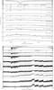 |
Fig. 1 UVES spectra over the sdM spectral sequence.The spectra are scaled to normalize the average flux to unity. The spectrum of the standard star EG 21 shows the location of telluric atmospheric features. |
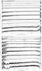 |
Fig. 1 continued. |
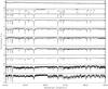 |
Fig. 1 continued. |
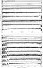 |
Fig. 2 continued. |
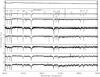 |
Fig. 2 continued. |
2.2. Molecular features
The optical spectra are dominated by molecular absorption bands from metal oxide species such as titanium oxide (TiO), vanadium oxide (VO), and hydrides such as CaH and H2O. They are the most significant opacity sources. However, due to the low metallicity of subdwarfs, they are TiO depleted. The primary effects are the strengthening of hydride bands and collision-induced absorption (CIA) by H2, and the broadening of atomic lines (Allard et al. 1997). Unlike TiO, which produces distinctive band heads degraded on the red, VO produces more diffuse absorption. CaH hydride bands are significant opacity sources, but decrease in relative strength and become saturated with decreasing temperature.
2.3. Atomic lines
All the observed M subdwarfs show strong alkali lines in the observed wavelength range. They are massively pressure broadened, as expected from their high-gravity surface. Atomic features such as Ca II, K I, Rb I, Na I, Ti I, and Mg I are visible throughout the sequence, and their lines are prominent in almost all of the spectra. However, in regions where strong atmospheric absorption is present, it is difficult to measure the intensities of these lines.
The Na I lines at 8183 Å and 8194 Å are clearly visible in all the observed spectra and become broadened from hotter to cooler M subdwarfs. In our setting they appear just at the red end of the lower chip of the blue arm. The K I lines are very narrow for early-type subdwarfs but become very wide and smooth in late-type subdwarfs. The K I resonance lines at 7665 Å and 7698 Å govern the spectral shape of cool subdwarf spectra. The equivalent width of these K I lines are of several hundred Å. The ionized Ca II triplet lines at 8498 Å, 8542 Å, and 8662 Å are very strong in all the observed spectra. Their detailed study by Mallik (1997) shows that their strengths depend on stellar parameters like luminosity, temperature, and metallicity. They are ideal candidates to study their sensitivity to various stellar parameters in cool stars. Although the lower levels of the Ca II triplet lines are populated radiatively and are not collision controlled, they have been identified as very good luminosity probes by Mallik (1997). They are relatively free from blends and are little contaminated by telluric lines. In contrast, the Na I lines at 8183 Å and 8195 Å, which have also been used as luminosity probes in cool stars, have several atmospheric absorption lines in their vicinity (Alloin & Bica 1989; Zhou 1991).
3. Model atmospheres
We used the most recent BT-Settl models that were partially published in a review by Allard et al. (2012). These atmosphere models are computed with the PHOENIX multi-purpose atmosphere code version 15.5 (Hauschildt et al. 1997; Allard et al. 2001), solving the radiative transfer in 1D spherical symmetry, with the classical assumption of: hydrostatic equilibrium, convection using the mixing-length theory, chemical equilibrium, and a sampling treatment of the opacities. The models use a mixing length as derived by the radiation hydrodynamic simulations of Ludwig et al. (2002, 2006), and Freytag et al. (2012).
Compared with previous models by Allard et al. (2001), the current version of the BT-Settl model atmosphere uses the BT2 water-vapor line list computed by Barber et al. (2006), TiO, VO, CaH line lists by Plez (1998), MgH by Weck et al. (2003) and Skory et al. (2003), FeH and CrH by Dulick et al. (2003) and Chowdhury et al. (2006), CO2 by Tashkun et al. (2004), H2 CIA by Borysow et al. (2001); Abel et al. (2011), and CO by Goorvitch & Chackerian (1994a,b), to mention the most important line lists. We also included the H2-He CIA from Borysow & Frommhold (1989) and Borysow et al. (1997), H2-H from Gustafsson et al. (2003), and H-He (at least in the most recent models) from Gustafsson & Frommhold (2001). Detailed profiles for the alkali lines were also used (Allard et al. 2007). The reference solar elemental abundances used in this version of the BT-Settl models those measured by Caffau et al. (2011).
In general, the Unsold (1968) approximation is used, with the general exception of Na I, Si I, Ca I, and Fe I, where we instead used the respective correction factors found by Gustafsson et al. (2008) for the atomic damping constants with a correction factor to the widths of 2.5 for the non-hydrogenic atoms (Valenti & Piskunov 1996). More accurate broadening data for neutral hydrogen collisions by Barklem et al. (2000) were included for several important atomic transitions such as the alkali, Ca I, and Ca II resonance lines. For molecular lines, we adopted average values (e. g.  1)⟩ H2O = 0.08 Pgas [ cm-1atm-1 ] for water vapor lines) from the HITRAN database (Rothman et al. 2009), which are scaled to the local gas pressure and temperature
 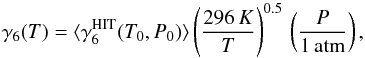 (1)with a single temperature exponent of 0.5, to be compared with values ranging mainly from 0.3 to 0.6 for water transitions studied by Gamache et al. (1996). The HITRAN database gives widths for broadening in air, but Bailey & Kedziora-Chudczer (2012) found that these agree in general within 10–20% with those for broadening by a solar-composition hydrogen-helium mixture.
The BT-Settl grid extends from Teff = 300 to 7000 K in steps of 100 K, log g = 2.5 to 5.5 in steps of 0.5, and [M/H] = − 2.5 to 0.0 in steps of 0.5, which accounts for alpha-element enrichment. The alpha enhancement was taken as [alpha/Fe] = − 0.4× [Fe/H] for 0 > [Fe/H] >−1 and 0.4 for metallicities <−1.0, which is also consistent with the choice of Gustafsson et al. (2008). These different prescriptions for alpha enhancement are rough estimates for the old thin disc and thick disc, respectively (see e.g. Neves et al. 2009, for a discussion on the abundance trends relative to Fe).
We linearly interpolated the grid at every 0.1 dex in log g and metallicity. For more details of the BT-Sett model atmosphere see Allard et al. (2012, 2013) and Rajpurohit et al. (2012). The synthetic colours and spectra were distributed with a resolution of around R = 100 000 via the PHOENIX web simulator2.
Figure 3 shows BT-Settl synthetic spectra varying Teff and [M/H]. Oxide bands that dominate in M dwarf spectra are weaker in the subdwarfs where the hydride bands dominate (Jao et al. 2008). They have complex and extensive band structures that leave no window for the true continuum and create a pseudo-continuum that only lets pass the strongest, often resonance atomic lines (Allard 1990; Allard & Hauschildt 1995). However, because of the lower metallicity of subdwarfs, the TiO bands are weaker, and the pseudo-continuum is brighter. This increases the contrast to the other opacities such as hydride bands and atomic lines, which feel the higher pressures of the deeper layers where they emerge from. We therefore see these molecular bands with more detaile and under more extreme gas pressure conditions than for M dwarfs.
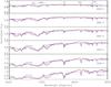 |
Fig. 3 BT-Settl synthetic spectra from 4000 K to 3000 K. The black, red, and blue lines represent [M/H] = 0.0, − 1.0, and −2.0, respectively. |
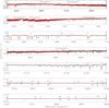 |
Fig. 4 UVES spectra of the sdM1 star LHS 158 (black) compared with the best-fit BT-Settl synthetic spectra (red). |
Although the models were computed for different [M/H] values, in the following we use [Fe/H] everywhere. Indeed, we use only the iron lines for the metallicity determinations so that in fact we determine a [Fe/H] value.
4. Comparison with model atmospheres
We perform a comparison between observed and synthetic spectra computed from the BT Settl model to derive the physical parameters of our sample. Furthermore, the comparison with observed spectra is very crucial to reveal the inaccuracy or incompleteness of the opacities used in the model. Figures 4 and 5 show the comparison of the best-fit model for an sdM1 and a usdM4.5 star.
4.1. Molecular bands
The spectra agree well and reproduce the specific strengths of the TiO band heads at 6600 Å, 6700 Å, 7050 Å,7680Å, and 8859 Å, and of the VO bands at 7000 Å, 7430 Å, and 7852 Å. The excellent match between models and observations over entire subdwarf sequence shows that the high-frequency pattern visible at this spectral resolution is the structure of the absorption band and not noise.
4.2. Atomic lines
The models predict the shape of the Na I doublet at 8194 Å and 8183 Å rather well but its strength is well fitted only poorly. In the sdM3.0 and later and in esdM, the observed lines are broader and shallower than those predicted by the models.
The qualitative behaviour of the K I doublet at 7665 Å and 7698 Å is well reproduced by the models, especially the strong pressure-broadening wings in the early sdM and esdM. In the sdM0, the cores of the observed K I lines are still visible as relatively narrow absorption minima embedded in wings extending a few tens to one hundred Å. This broader absorption component becomes saturated in sdM7 spectrum. The models also show this effect but do not reproduce it perfectly. This may be an indication (i) that the models do not yet produce correct densities of the neutral alkali metals in the uppermost part of the atmosphere, since the central parts of the lines form in the highest layers of the atmosphere, especially in the early sdM and esdM where alkali metals are not depleted strongly (Johnas et al. 2007); or (ii) that the depth of atomic lines can only be reproduced when accounting for a magnetic field and Zeeman broadening (Deen 2013).
The models reproduce the strength and wings of Ca II triplet lines at 8498 Å, 8542 Å, and 8662 Å very well. We also have a good fit to the Ti I lines. They are located between 8400 Å to 9700 Å and belong to low-energy transitions that appear to be visible in such cool atmospheres (see also Reiners & Basri 2006).
Absorption lines of Rb appear in spectra later than sdM7.0. They become stronger and wider towards lower temperature. Given the fact that they are embedded in pseudo-continua that are not always a good fit to the data, the behaviour of the two Rb lines at 7800 Å and 7948 Å is very well reproduced by the models.
4.3. Stellar parameter determination
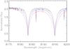 |
Fig. 6 BT-Settl synthetic spectra with Teff of 3500 K and varying log g = 4.5 (black), 5.0 (blue), 5.5 (red). The effect of gravity and pressure broadening on the sodium doublet is clearly visible. |
The analysis using synthetic spectra requires the specification of several input parameters: effective temperature, surface gravity, and the overall metallicity with respect to the Sun. We first convolved the synthetic spectrum with a Gaussian kernel at the observed resolution and then interpolated the result with the observation. We performed a χ2 fitting between the grid of synthetic spectra and observed spectra in the wavelength range 6400 Å to 8900 Å, as shown by Önehag et al. (2012). We excluded the spectral region between 6860 to 6960 Å, 7550 to 7650 Å, and 8200 to 8430 Å because of atmospheric absorption. We let all the stellar parameters (Teff, [Fe/H], log g) vary.
The minimum χ2 value gives the best-fit parameters and their error bars were derived by allowing a 5% deviation of the χ2 value from its minimum value. The acceptable parameters were finally inspected by comparing them with the observed spectra.
The TiO system at 6600 Å, 6700 Å, and 7100 Å is highly sensitive to Teff (increasing in strength with decreasing Teff) and rather insensitive to variation in gravity. At a given Teff, the band strengths change only slightly even for a large 0.5 change in gravity (in the log g = 4.5 − 5.5 range expected for low-mass stars). At a given gravity, however, they vary significantly over a change of only 100 K in Teff.
The surface gravity determination was checked on the width of gravity-sensitive atomic lines such as the K I and Na I doublets (see Fig. 6) as well as on the relative strength of metal-hydride bands such as CaH. The K I doublet at 7665 Å and 7699 Å and the Na I lines at 8183 Å and 8194 Å are particularly useful gravity discriminants for M dwarfs and subdwarfs. The overall line strength (central depth and equivalent width) increases with gravity as the decreasing ionization ratio due to higher electron pressure leaves more neutral alkali lines in the deeper atmosphere (Reiners 2005). The width of the damping wings in addition increases due to the stronger pressure broadening, mainly by H2, He, and H I collisions.
We also checked the metallicity determination on the spectral interval from 8440 Å to 8900 Å where molecular absorptions are lower and atomic lines appear clearly (see Fig. 7). The synthetic spectrum represents the line profiles fairly well for elemental species such as Ti, I Fe I, Ca II, and Mg I. The best-fit parameters (Teff, log g, [Fe/H]) are given in Table 2.
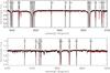 |
Fig. 7 UVES spectrum of the sdM1 star LHS 158 (black) and the best-fit BT Settl synthetic spectrum (red). The strong atomic features are highlighted. |
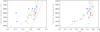 |
Fig. 8 Effective temperature versus near-infrared colours of our sample of subdwarfs. The different colours stand for different metallicities: [Fe/H] = −0.5 to −0.7 dex (red), [Fe/H] = −1.0 to −1.2 dex (green), [Fe/H] = − 1.3 to −1.6 dex (blue), [Fe/H] = −1.7 dex (brown). The lines are from evolution models from Baraffe et al. (1998) at different metallicities (red: −0.5 dex, green: −1.0 dex, blue: −1.5 dex, brown: − 2.0 dex) assuming an age of 10 Gyr. |
5. Discussion
The effective temperature versus near-infrared colours are shown in Fig. 8. The expected relations from evolution models (Baraffe et al. 1997, 1998) assuming an age of 10 Gyr and varying metallicities are also superimposed. The colours stand for different metallicities. The plot shows discrepancies between the models and our observations. It shows that the metallicities determined from the high-resolution spectral features are inconsistent with those we would infer from near-infrared colours. This inconsistency may be due to uncertainties in the CIA opacities or to outdated model interiors. It shows that broad-band colours are not sufficient to determine the parameters of M subdwarfs.
The relation of effective temperature versus spectral-type is shown in Fig. 9. The relation determined using UVES sample is compared with the Teff scale of M dwarfs determined by Rajpurohit et al. (2013). The Teff of subdwarfs is 200–300 K higher than Teff of M dwarfs for the same spectral type except for hot temperatures. This is expected since the TiO bands are depleted with decreasing metallicity, and as a result, the pseudo-continuum is brighter and the flux is emitted from the hot deeper layer. A comparison with the earlier work from Gizis (1997) is also shown. Gizis (1997) determined the temperature by comparing the low-resolution optical spectra of a sample of sdM and esdM with the NextGen model atmosphere grid by Allard et al. (1997). The Teff for subdwarfs agrees within 100 K. This difference is due to the incompleteness of the TiO and water vapor line lists used in the NextGen model atmospheres compared with the new BT-Settl models. Furthermore, this work allows us to extend the relation to the coolest M subdwarfs.
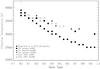 |
Fig. 9 Relation of the effective temperature of subdwarfs versus spectral type from our sample (filled symbols) compared with those from Gizis (1997, open symbols) and the M dwarf Teff scale from Rajpurohit et al. (2013, filled circles). |
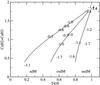 |
Fig. 10 CaH2+CaH3 versus TiO5 diagram for our sample. The labels indicate our metallicity determination. The lines are defined by Lépine et al. (2007). They show the different regions in the diagram where sdM, esdM, and usdM stars are expected to be. |
We compiled from the literature the spectral indices of TiO5, CaH2, and CaH3 computed from TiO and CaH band strengths on low-resolution spectra (see Table 1). The last column gives the references for spectral types and spectral indices. When possible, we took both the spectral type and the indices from the same paper. We note that the spectral indices may vary over several subtypes for some of the stars from one author to the other. Since Jao et al. (2008) did not give new spectral types in the scheme developed by Gizis (1997) that was extended by Lépine et al. (2007) (sd, esd, usd), which we used, we adopted the indices from Jao et al. (2008) and assigned sdM types only when no indices were available from the papers providing an sd, esd, usd classification.
Figure 10 shows the CaH2+CaH3 versus TiO5. Lépine et al. (2003b) showed that such a diagram is useful to distinguish between the different object classes, sdM, esdM, and usdM. Our metallicity determinations are labelled in the diagram. It shows that the metallicity decreases from sdM to usdM as expected.
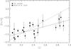 |
Fig. 11 ζ parameter defined by Lépine et al. (2007) versus metallicity diagram. The circles show our sample and the solid black line is the linear-square regression. The sample from Woolf et al. (2009) is superimposed (squares) as well as their derived relation (dashed line). |
We also derived the ζ parameter as defined by Lépine et al. (2007). This ζ parameter is a combination of the TiO5, CaH2, and CaH3 spectral indices. Woolf et al. (2009) used a sample of 12 esdM and usdM with known metallicities to derive a correlation between ζ and the metallicity, and showed that it can be used as a metallicity indicator. We plot the metallicity of our stars versus ζ (Fig. 11) and superimpose the sample from Woolf et al. (2009) as well as their derived correlation (dashed line). We also define a similar correlation (solid line) using our sample, ![Mathematical equation: \begin{eqnarray*} \rm [Fe/H] = 1.19 \zeta - 1.75. \end{eqnarray*}](/articles/aa/full_html/2014/04/aa22881-13/aa22881-13-eq36.png) Although the relation shows a strong dispersion in both samples, our metallicity determinations tend to be lower on average. This can be due to the different spectral indices adopted, or to the use of different atmosphere models. LHS 161, the only common star in both samples, illustrates the first assumption. Our metallicity determination (− 1.2 dex) agrees with that of Woolf et al. (2009), (− 1.3 dex) but the spectral indices adopted are very different: we used ζ = 0.07 from the indices of Gizis (1997) whereas Woolf et al. (2009) used ζ = 0.41 from the indices of Jao et al. (2008). Furthermore, Woolf et al. (2009) used NextGen models.
Although the relation shows a strong dispersion in both samples, our metallicity determinations tend to be lower on average. This can be due to the different spectral indices adopted, or to the use of different atmosphere models. LHS 161, the only common star in both samples, illustrates the first assumption. Our metallicity determination (− 1.2 dex) agrees with that of Woolf et al. (2009), (− 1.3 dex) but the spectral indices adopted are very different: we used ζ = 0.07 from the indices of Gizis (1997) whereas Woolf et al. (2009) used ζ = 0.41 from the indices of Jao et al. (2008). Furthermore, Woolf et al. (2009) used NextGen models.
6. Conclusion
We presented a high-resolution optical spectral atlas for a sample of 18 M subdwarfs and 3 K subdwarfs, including 5 esdK,1 esdM, and 2 usdM3. We described various atomic and molecular features that appear in the spectra and their evolution with decreasing effective temperature and metallicity. We used the most recent BT-Settl model atmospheres, with revised solar abundances, to determine the scaled solar abundances of the subdwarfs. We compared them with the synthetic spectra produced by the BT-Settl atmosphere models and derived their fundamental stellar parameters. The accuracy of the atmospheric models involved in the metallicity determination can be inferred by looking at the fit to the individual atomic and molecular lines. These high-resolution spectra allowed us to separate the atmospheric parameters (effective temperature, gravity, metallicity), which is not possible when using broad-band photometry.
We determined the relation of effective temperature versus spectral type of M-subdwarfs and compared it with the previous study from Gizis (1997). Our relation agrees within 100 K and extends to the cooler spectral sequence. This work also contributes to calibrating the relation between metallicity and photometric colours and molecular band strengths. With this calibration, it will be possible to estimate the metallicity of a large sample of subdwarfs and obtain a meaningful statistical analysis.
The next step of this work is to investigate the effect of different alpha enhancements on the spectral energy distribution and the spectral-line strengths of M subdwarfs. This effect is expected to be as important as the revised oxygen abundances were to make the models fit solar metallicity M dwarfs. This is a limitation of the models because M subdwarfs are divided into two regimes, each with a rough prescription of alpha enhancements. More realistic abundance trends need to be applied to the models (Neves et al. 2009; Adibekyan et al. 2012). This atlas is appropriate for testing these prescriptions and their effect on the atmosphere spectra because they are precise enough to allow us to derive elemental abundances.
Standard temperature 296 K and pressure 1 atm.
The atlas will be made public through the Virtual Observatory tools.
Acknowledgments
We acknowledge observing support from the ESO staff. We acknowledge financial support from “Programme National de Physique Stellaire” (PNPS) of CNRS/INSU, France. We thank the referee J. Gizis for his useful comments on the paper.
References
- Abel, M., Frommhold, L., Li, X., & Hunt, K. L. C. 2011, in 66th International Symp. Molecular Spectroscopy, Ohio State University [Google Scholar]
- Adibekyan, V. Z., Sousa, S. G., Santos, N. C., et al. 2012, A&A, 545, A32 [NASA ADS] [CrossRef] [EDP Sciences] [Google Scholar]
- Allard, F. 1990, Ph.D. Thesis, Ruprecht Karls Univ. Heidelberg [Google Scholar]
- Allard, F., & Hauschildt, P. H. 1995, ApJ, 445, 433 [NASA ADS] [CrossRef] [Google Scholar]
- Allard, F., Hauschildt, P. H., Alexander, D. R., & Starrfield, S. 1997, ARA&A, 35, 137 [NASA ADS] [CrossRef] [Google Scholar]
- Allard, F., Hauschildt, P. H., Alexander, D. R., Tamanai, A., & Schweitzer, A. 2001, ApJ, 556, 357 [NASA ADS] [CrossRef] [Google Scholar]
- Allard, N. F., Kielkopf, J. F., & Allard, F. 2007, EPJ D, 44, 507 [Google Scholar]
- Allard, F., Homeier, D., & Freytag, B. 2012, Roy. Soc. London Philos. Trans. Ser. A, 370, 2765 [Google Scholar]
- Allard, F., Homeier, D., Freytag, B., et al. 2013, Mem. Soc. Astron. It. Suppl., 24, 128 [Google Scholar]
- Alloin, D., & Bica, E. 1989, A&A, 217, 57 [NASA ADS] [Google Scholar]
- Asplund, M., Grevesse, N., Sauval, A. J., & Scott, P. 2009, ARA&A, 47, 481 [NASA ADS] [CrossRef] [Google Scholar]
- Bailey, J., & Kedziora-Chudczer, L. 2012, MNRAS, 419, 1913 [NASA ADS] [CrossRef] [Google Scholar]
- Baraffe, I., Chabrier, G., Allard, F., & Hauschildt, P. H. 1997, A&A, 327, 1054 [NASA ADS] [Google Scholar]
- Baraffe, I., Chabrier, G., Allard, F., & Hauschildt, P. H. 1998, A&A, 337, 403 [NASA ADS] [Google Scholar]
- Barber, R. J., Tennyson, J., Harris, G. J., & Tolchenov, R. N. 2006, MNRAS, 368, 1087 [NASA ADS] [CrossRef] [Google Scholar]
- Barklem, P. S., Piskunov, N., & O’Mara, B. J. 2000, A&A, 363, 1091 [NASA ADS] [Google Scholar]
- Bean, J. L., Sneden, C., Hauschildt, P. H., Johns-Krull, C. M., & Benedict, G. F. 2006, ApJ, 652, 1604 [NASA ADS] [CrossRef] [Google Scholar]
- Bidelman, W. P. 1985, ApJS, 59, 197 [NASA ADS] [CrossRef] [Google Scholar]
- Bonfils, X., Forveille, T., Delfosse, X., et al. 2005, A&A, 443, L15 [NASA ADS] [CrossRef] [EDP Sciences] [Google Scholar]
- Borysow, A., & Frommhold, L. 1989, ApJ, 341, 549 [NASA ADS] [CrossRef] [Google Scholar]
- Borysow, A., Jorgensen, U. G., & Zheng, C. 1997, A&A, 324, 185 [NASA ADS] [Google Scholar]
- Borysow, A., Jørgensen, U. G., & Fu, Y. 2001, J. Quant. Spectr. Rad. Transf., 68, 235 [NASA ADS] [CrossRef] [Google Scholar]
- Burgasser, A. J., & Kirkpatrick, J. D. 2006, ApJ, 645, 1485 [NASA ADS] [CrossRef] [Google Scholar]
- Burgasser, A. J., Kirkpatrick, J. D., Burrows, A., et al. 2003, ApJ, 592, 1186 [NASA ADS] [CrossRef] [Google Scholar]
- Caffau, E., Ludwig, H.-G., Steffen, M., Freytag, B., & Bonifacio, P. 2011, Sol. Phys., 268, 255 [NASA ADS] [CrossRef] [Google Scholar]
- Casagrande, L., Flynn, C., & Bessell, M. 2008, MNRAS, 389, 585 [NASA ADS] [CrossRef] [MathSciNet] [Google Scholar]
- Chowdhury, P. K., Merer, A. J., Rixon, S. J., Bernath, P. F., & Ram, R. S. 2006, Phys. Chem. Chem. Phys., 8, 822 [Google Scholar]
- Dawson, P. C., & De Robertis, M. M. 2000, AJ, 120, 1532 [NASA ADS] [CrossRef] [Google Scholar]
- Deen, C. P. 2013, AJ, 146, 51 [NASA ADS] [CrossRef] [Google Scholar]
- Dekker, H., D’Odorico, S., Kaufer, A., Delabre, B., & Kotzlowski, H. 2000, in SPIE Conf. Ser. 4008, eds. M. Iye, & A. F. Moorwood, 534 [Google Scholar]
- Digby, A. P., Hambly, N. C., Cooke, J. A., Reid, I. N., & Cannon, R. D. 2003, MNRAS, 344, 583 [NASA ADS] [CrossRef] [Google Scholar]
- Dulick, M., Bauschlicher, Jr., C. W., Burrows, A., et al. 2003, ApJ, 594, 651 [NASA ADS] [CrossRef] [Google Scholar]
- Freytag, B., Steffen, M., Ludwig, H.-G., et al. 2012, J. Comp. Phys., 231, 919 [Google Scholar]
- Gamache, R. R., Lynch, R., & Brown, L. R. 1996, J. Quant. Spectr. Rad. Transf., 56, 471 [NASA ADS] [CrossRef] [Google Scholar]
- Gizis, J. E. 1997, AJ, 113, 806 [NASA ADS] [CrossRef] [Google Scholar]
- Goorvitch, D., & Chackerian, Jr., C. 1994a, ApJS, 91, 483 [NASA ADS] [CrossRef] [Google Scholar]
- Goorvitch, D., & Chackerian, Jr., C. 1994b, ApJS, 92, 311 [NASA ADS] [CrossRef] [Google Scholar]
- Gustafsson, M., & Frommhold, L. 2001, ApJ, 546, 1168 [NASA ADS] [CrossRef] [Google Scholar]
- Gustafsson, M., Kristensen, L. E., Clénet, Y., et al. 2003, A&A, 411, 437 [NASA ADS] [CrossRef] [EDP Sciences] [Google Scholar]
- Gustafsson, B., Edvardsson, B., Eriksson, K., et al. 2008, A&A, 486, 951 [NASA ADS] [CrossRef] [EDP Sciences] [Google Scholar]
- Hauschildt, P. H., Baron, E., & Allard, F. 1997, ApJ, 483, 390 [NASA ADS] [CrossRef] [Google Scholar]
- Jao, W.-C., Henry, T. J., Beaulieu, T. D., & Subasavage, J. P. 2008, AJ, 136, 840 [NASA ADS] [CrossRef] [Google Scholar]
- Johnas, C. M. S., Hauschildt, P. H., Schweitzer, A., et al. 2007, A&A, 475, 1039 [NASA ADS] [CrossRef] [EDP Sciences] [Google Scholar]
- Kirkpatrick, J. D., Looper, D. L., Burgasser, A. J., et al. 2010, ApJS, 190, 100 [NASA ADS] [CrossRef] [Google Scholar]
- Lépine, S., Rich, R. M., & Shara, M. M. 2003a, AJ, 125, 1598 [NASA ADS] [CrossRef] [Google Scholar]
- Lépine, S., Shara, M. M., & Rich, R. M. 2003b, AJ, 126, 921 [NASA ADS] [CrossRef] [Google Scholar]
- Lépine, S., Rich, R. M., & Shara, M. M. 2007, ApJ, 669, 1235 [NASA ADS] [CrossRef] [Google Scholar]
- Ludwig, H.-G., Allard, F., & Hauschildt, P. H. 2002, A&A, 395, 99 [NASA ADS] [CrossRef] [EDP Sciences] [Google Scholar]
- Ludwig, H.-G., Allard, F., & Hauschildt, P. H. 2006, A&A, 459, 599 [NASA ADS] [CrossRef] [EDP Sciences] [Google Scholar]
- Mallik, S. V. 1997, A&AS, 124, 359 [NASA ADS] [CrossRef] [EDP Sciences] [Google Scholar]
- Neves, V., Santos, N. C., Sousa, S. G., Correia, A. C. M., & Israelian, G. 2009, A&A, 497, 563 [NASA ADS] [CrossRef] [EDP Sciences] [Google Scholar]
- Önehag, A., Heiter, U., Gustafsson, B., et al. 2012, A&A, 542, A33 [NASA ADS] [CrossRef] [EDP Sciences] [Google Scholar]
- Plez, B. 1998, A&A, 337, 495 [NASA ADS] [Google Scholar]
- Rajpurohit, A. S., Reylé, C., Schultheis, M., et al. 2012, A&A, 545, A85 [NASA ADS] [CrossRef] [EDP Sciences] [Google Scholar]
- Rajpurohit, A. S., Reylé, C., Allard, F., et al. 2013, A&A, 556, A15 [NASA ADS] [CrossRef] [EDP Sciences] [Google Scholar]
- Reiners, A. 2005, Astron. Nachr., 326, 930 [NASA ADS] [CrossRef] [Google Scholar]
- Reiners, A., & Basri, G. 2006, AJ, 131, 1806 [NASA ADS] [CrossRef] [Google Scholar]
- Reiners, A., Homeier, D., Hauschildt, P. H., & Allard, F. 2007, A&A, 473, 245 [NASA ADS] [CrossRef] [EDP Sciences] [Google Scholar]
- Reylé, C., Scholz, R.-D., Schultheis, M., Robin, A. C., & Irwin, M. 2006, MNRAS, 373, 705 [NASA ADS] [CrossRef] [Google Scholar]
- Rodgers, A. W., & Eggen, O. J. 1974, PASP, 86, 742 [NASA ADS] [CrossRef] [Google Scholar]
- Rothman, L. S., Gordon, I. E., Barbe, A., et al. 2009, J. Quant. Spectr. Rad. Transf., 110, 533 [NASA ADS] [CrossRef] [Google Scholar]
- Scholz, R.-D., Ibata, R., Irwin, M., et al. 2002, MNRAS, 329, 109 [NASA ADS] [CrossRef] [Google Scholar]
- Scholz, R.-D., Lehmann, I., Matute, I., & Zinnecker, H. 2004, A&A, 425, 519 [NASA ADS] [CrossRef] [EDP Sciences] [Google Scholar]
- Schweitzer, A., Scholz, R.-D., Stauffer, J., Irwin, M., & McCaughrean, M. J. 1999, A&A, 350, L62 [NASA ADS] [Google Scholar]
- Skory, S., Weck, P. F., Stancil, P. C., & Kirby, K. 2003, ApJS, 148, 599 [NASA ADS] [CrossRef] [Google Scholar]
- Skrutskie, M. F., Cutri, R. M., Stiening, R., et al. 2006, AJ, 131, 1163 [NASA ADS] [CrossRef] [Google Scholar]
- Tashkun, S. A., Perevalov, V. I., Teffo, J.-L., et al. 2004, Proc. SPIE, 5311, 102 [NASA ADS] [CrossRef] [Google Scholar]
- Tinney, C. G., & Reid, I. N. 1998, MNRAS, 301, 1031 [NASA ADS] [CrossRef] [Google Scholar]
- Unsold, A. 1968, Physik der Sternatmospharen, MIT besonder Berucksichtigung der Sonne (Berlin, New York: Springer Verlag) [Google Scholar]
- Valenti, J. A., & Piskunov, N. 1996, A&AS, 118, 595 [NASA ADS] [CrossRef] [EDP Sciences] [Google Scholar]
- Weck, P. F., Schweitzer, A., Stancil, P. C., Hauschildt, P. H., & Kirby, K. 2003, ApJ, 584, 459 [NASA ADS] [CrossRef] [Google Scholar]
- Woolf, V. M., & Wallerstein, G. 2005, MNRAS, 356, 963 [NASA ADS] [CrossRef] [Google Scholar]
- Woolf, V. M., Lépine, S., & Wallerstein, G. 2009, PASP, 121, 117 [NASA ADS] [CrossRef] [Google Scholar]
- Zhou, X. 1991, A&A, 248, 367 [NASA ADS] [Google Scholar]
All Figures
|
Fig. 1 UVES spectra over the sdM spectral sequence.The spectra are scaled to normalize the average flux to unity. The spectrum of the standard star EG 21 shows the location of telluric atmospheric features. |
| In the text | |
|
Fig. 1 continued. |
| In the text | |
|
Fig. 1 continued. |
| In the text | |
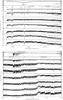 |
Fig. 2 Same as Fig. 1 for esdM and usdM stars. |
| In the text | |
|
Fig. 2 continued. |
| In the text | |
|
Fig. 2 continued. |
| In the text | |
|
Fig. 3 BT-Settl synthetic spectra from 4000 K to 3000 K. The black, red, and blue lines represent [M/H] = 0.0, − 1.0, and −2.0, respectively. |
| In the text | |
|
Fig. 4 UVES spectra of the sdM1 star LHS 158 (black) compared with the best-fit BT-Settl synthetic spectra (red). |
| In the text | |
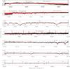 |
Fig. 5 Same as Fig. 4 for the usdM4.5 star LHS 1032. |
| In the text | |
|
Fig. 6 BT-Settl synthetic spectra with Teff of 3500 K and varying log g = 4.5 (black), 5.0 (blue), 5.5 (red). The effect of gravity and pressure broadening on the sodium doublet is clearly visible. |
| In the text | |
|
Fig. 7 UVES spectrum of the sdM1 star LHS 158 (black) and the best-fit BT Settl synthetic spectrum (red). The strong atomic features are highlighted. |
| In the text | |
|
Fig. 8 Effective temperature versus near-infrared colours of our sample of subdwarfs. The different colours stand for different metallicities: [Fe/H] = −0.5 to −0.7 dex (red), [Fe/H] = −1.0 to −1.2 dex (green), [Fe/H] = − 1.3 to −1.6 dex (blue), [Fe/H] = −1.7 dex (brown). The lines are from evolution models from Baraffe et al. (1998) at different metallicities (red: −0.5 dex, green: −1.0 dex, blue: −1.5 dex, brown: − 2.0 dex) assuming an age of 10 Gyr. |
| In the text | |
|
Fig. 9 Relation of the effective temperature of subdwarfs versus spectral type from our sample (filled symbols) compared with those from Gizis (1997, open symbols) and the M dwarf Teff scale from Rajpurohit et al. (2013, filled circles). |
| In the text | |
|
Fig. 10 CaH2+CaH3 versus TiO5 diagram for our sample. The labels indicate our metallicity determination. The lines are defined by Lépine et al. (2007). They show the different regions in the diagram where sdM, esdM, and usdM stars are expected to be. |
| In the text | |
|
Fig. 11 ζ parameter defined by Lépine et al. (2007) versus metallicity diagram. The circles show our sample and the solid black line is the linear-square regression. The sample from Woolf et al. (2009) is superimposed (squares) as well as their derived relation (dashed line). |
| In the text | |
Current usage metrics show cumulative count of Article Views (full-text article views including HTML views, PDF and ePub downloads, according to the available data) and Abstracts Views on Vision4Press platform.
Data correspond to usage on the plateform after 2015. The current usage metrics is available 48-96 hours after online publication and is updated daily on week days.
Initial download of the metrics may take a while.