| Issue |
A&A
Volume 563, March 2014
|
|
|---|---|---|
| Article Number | A9 | |
| Number of page(s) | 6 | |
| Section | Interstellar and circumstellar matter | |
| DOI | https://doi.org/10.1051/0004-6361/201323145 | |
| Published online | 25 February 2014 | |
XMM-Newton observation of the Galactic supernova remnant W51C (G49.1–0.1)⋆
Institut für Astronomie und Astrophysik, Universität Tübingen Sand 1 72076 Tübingen Germany
e-mail:
sasaki@astro.uni-tuebingen.de
Received: 28 November 2013
Accepted: 15 January 2014
Context. The supernova remnant (SNR) W51C is a Galactic object located in a strongly inhomogeneous interstellar medium with signs of an interaction of the SNR blast wave with dense molecular gas.
Aims. Diffuse X-ray emission from the interior of the SNR can reveal element abundances in the different emission regions and shed light on the type of supernova (SN) explosion and its progenitor. The hard X-ray emission helps to identify possible candidates for a pulsar formed in the SN explosion and for its pulsar wind nebula (PWN).
Methods. We have analysed X-ray data obtained with XMM-Newton. Spectral analyses in selected regions were performed.
Results. Ejecta emission in the bright western part of the SNR, located next to a complex of dense molecular gas, was confirmed. The Ne and Mg abundances suggest a massive progenitor with a mass of >20 M⊙. Two extended regions emitting hard X-rays were identified (corresponding to the known sources [KLS2002] HX3 west and CXO J192318.5+140305 discovered with ASCA and Chandra, respectively), each of which has an additional point source inside and shows a power-law spectrum with Γ ≈ 1.8. Based on their X-ray emission, both sources can be classified as PWN candidates.
Key words: shock waves / HII regions / X-rays: ISM / X-rays: individuals: individual: SNR W51C
© ESO, 2014
1. Introduction
Supernova remnants (SNRs) are galactic objects that are formed after a supernova (SN) explosion at the end of the life of a star. An SN explosion instantaneously releases energy and matter into the ambient interstellar medium (ISM), carving out new structures inside a galaxy and enriching it with elements that were formed inside the progenitor star and in the explosion. In the shock waves of SNRs, particles can be accelerated and become Galactic cosmic rays. Multi-frequency studies of SNRs from radio to X-rays, in some cases even to γ-rays, help to understand the physics of the shock waves and the interaction between the SNR and the ISM.
The SNR W51C (G49.1–0.1) is a Galactic SNR in the W51 complex, an extended radio source at the tangential point of the Sagittarius arm. The W51 complex comprises two additional structures, W51A and W51B, which both harbour compact H ii regions. High-velocity molecular gas that runs almost parallel to the Galactic plane, known as the high-velocity stream (Mufson & Liszt 1979), has been detected on the western side of the SNR. Located in an area with a large number of H ii regions and dense molecular gas, W51C is a prime example of the interaction of an SNR blast wave with the multi-phase interstellar medium in our Galaxy.
The radio continuum of SNR W51C shows a thick arc-like structure with an extent of about 30′ (Copetti & Schmidt 1991; Subrahmanyan & Goss 1995). It is open to the north and its projected western edge coincides with W51B. The distance of 6 kpc to the SNR has been estimated from molecular-line observations (Koo & Moon 1997a,b; Green et al. 1997) and places it behind the ridge of molecular gas at 5.6 kpc. Assuming a Sedov model, Koo et al. (1995) derived an SNR age of ~3 × 10⁴ yr.
On its western side, where W51C merges with W51B in the radio image, shocked atomic H i was found (Koo & Heiles 1991). Furthermore, Koo & Moon (1997b) found CO and HCO+ emission, probably arising from molecules destroyed by a fast dissociative shock and reformed behind the shock front (Koo & Moon 1997a). Masers at 1720 MHz (OH) have also been found in W51C, between the SNR and the high-velocity stream of molecular gas (Green et al. 1997); OH (1720 MHz) emission, unaccompanied by maser emission from other OH ground-state transitions, is thought to arise in cooling gas behind non-dissociative shocks and is used to locate the site of shock-cloud interactions.
Diffuse X-ray emission was observed from W51B and W51C with the Einstein Imaging Proportional Counter (Seward 1990) and the Position Sensitive Proportional Counter (PSPC) of the Röntgen Satellite (ROSAT) mainly below 2 keV (Koo et al. 1995). The X-ray shell of W51C in the east and the western diffuse X-ray emission match the radio shell, while the emission gap observed in the soft X-rays between the bright central region and the western part coincides with W51B (see Fig. 1). Koo et al. (2002, hereafter KLS2002) derived a temperature of ~0.3 keV from data taken with the Advanced Satellite for Cosmology and Astrophysics (ASCA) for the central soft SNR emission, assuming thermal emission in collisional ionisation equilibrium. The hard (2.6−6.0 keV) X-ray image of ASCA is very different from the ROSAT image with the brightest regions seeming to be associated with compact H ii regions.
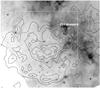 |
Fig. 1 A Midcourse Space Experiment (MSX, Egan et al. 2003) image in the infrared taken at 8.3 μm, together with ROSAT PSPC (0.1–2.4 keV) contours. The MSX image shows the emission from interstellar dust. The white cross marks the position of the OH (1720 MHz) masers. The white box indicates the field of the sky shown in Fig. 2. |
The remnant W51C is very likely the result of a core-collapse SN and should have an associated compact object. Images taken with the Chandra Advanced CCD Imaging Spectrometer (ACIS) in the soft band (0.3−2.1 keV, Koo et al. 2005) show several X-ray bright clumps. The spectra of the diffuse emission suggest an enhanced abundance of sulfur. In the hard band (2.1−10.0 keV), the point-like source CXO J192318.5+140305 was found, which is surrounded by an extended emission, making it a likely candidate for a pulsar wind nebula (PWN). This structure is similar to PWNe associated with several other SNRs, which all have a ~1 pc diameter bright core with a central pulsar or a point source. There is an indication of an unusual hardening at the ends of the envelope of this source in the Chandra data, but uncertainties are large. Its spectrum can be fitted with a power-law model (Γ = 1.8 ± 0.3, Koo et al. 2005). Recently, Hanabata et al. (2013) presented the results of a study of the inner parts of the SNR W51C performed with the Suzaku X-ray Imaging Spectrometer (XIS).
At higher energies γ-ray emission from the W51C region has been detected with the Large Area Telescope (LAT) on board Fermi (Abdo et al. 2009), the High Energy Stereoscopic System (H.E.S.S.)1, and the MAGIC telescopes (Aleksić et al. 2012). The GeV emission observed with Fermi is extended and seems to be consistent with the radio and X-ray extent of the remnant.
In this paper we present the analysis of the central part of the SNR W51C from a deep observation with the X-ray Multi-Mirror Mission (XMM-Newton, Jansen et al. 2001).
2. Data
The SNR W51C was observed with XMM-Newton on April 8, 2009, (obs. ID 0554690101) with the European Photon Imaging Cameras (EPICs, Strüder et al. 2001; Turner et al. 2001) as prime instruments using the medium filters. We used HEASOFT ver. 6.12 and the XMM-Newton Science Analysis System ver. 12.0.0 to analyse the data.
Since the emission from the SNR W51C fills almost the entire field of view (FOV) of the EPICs, we used the XMM-Newton Extended Source Analysis Software (ESAS)2 to analyse the data. Using ESAS, we filtered out bad time intervals caused by soft proton flares, resulting in good exposures of 40, 51, and 54 ks for EPIC-pn, MOS1, and MOS2, respectively. In addition, we checked whether any CCD of the MOS detectors was in an anomalous state. Since CCD4 of MOS1 showed an enhancement in the background below 1 keV and was therefore in an anomalous state3, this CCD was excluded from further analysis. The filtered events were used to perform source detection and create data with events of the extended emission. For further analysis, we selected single and double pixel events (PATTERN = 0 to 4) for the EPIC-pn and single to quadruple-pixel events (PATTERN = 0 to 12) for the EPIC-MOS1 and MOS2. To remove the detector background, data taken with the filter wheel closed (FWC) were binned to images and subtracted from the images of the observation after rescaling the FWC image using the count rates in the corners of the detectors, which are not exposed to the sky.
We are primarily interested in the extended diffuse emission of the SNR. Therefore, we ran the ESAS routines cheese (or cheese-bands for processing multiple energy bands) to detect point sources, which can then be removed in the following steps. These routines run source detection and create lists and masks of the detected point sources. The masks are used to remove the point sources from the images and the list of detected sources is used to exclude the sources in the extraction regions for spectral analysis. For the source detection we used a flux threshold of 1014 erg cm-2 s-1, a signal-to-noise ratio of 2, and a minimum separation of 40′′ for the point sources. In total, 48 point sources were found in the FOV, which we excluded when creating images and extracting spectra. We only checked the spectra and counterparts of the potential pulsar candidates, i.e. hard X-ray sources with associated hard extended emission around them (see Sect. 3.2).
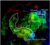 |
Fig. 2 Three-colour image of the mosaic images (red: 0.3–1.0 keV, green: 1.0–2.0 keV, blue: 2.0–8.0 keV). Extraction regions used for the spectral analysis are shown. Point sources are removed. |
To obtain deep images of the SNR in different energy bands, the images of the EPIC-pn and MOS1 and 2 were merged and divided by exposure maps, which take the vignetting effects into account. Figure 2 shows a three-colour presentation of the images in the bands 0.3−1.0 keV (red), 1.0−2.0 keV (green), and 2.0−8.0 keV (blue). These images, which are shown in logarithmic scale, were adaptively smoothed and then smoothed again using a Gaussian kernel of the size of 5 pixels for a better presentation of the faint diffuse emission. The holes in the images resulting from excluding point sources are not filled. The mosaicing of the three EPICs and the adaptive smoothing even out most of the holes as well as the chip gaps as can be seen in Fig. 2.
Using these images, extraction regions for the spectral analysis were defined based on surface brightness and X-ray colour (for details see Sect. 3). The spectra were rebinned with a minimum of 50 counts per bin. For a comparison of the distribution of the X-ray emission and the surrounding colder medium, we also downloaded an image from the Midcourse Space Experiment (MSX, see Fig.1, Egan et al. 2003). To estimate the local X-ray background, a background extraction region was defined north of the SNR emission. The fainter regions in the east to south-east or in the west are not appropriate as this is where the blast wave emission is expected. The background spectra were scaled to the source spectra using the areas of the extraction regions, taking into account that CCD4 in anomalous state and CCD6, which was damaged after being hit by a micrometeorite, are excluded for MOS1.
3. Spectral analysis
The spectra were analysed using the X-ray spectral fitting package XSPEC Ver. 12.8.1 and the atomic data base AtomDB 2.0.24. The emission of the SNR fills most of the FOV of the analysed observation. We divided the data into regions that are likely to have emission of similar nature based on the images in the broad band and the three-colour image (Fig. 2). Unfortunately, the statistics of the data were not high enough to analyse small regions. We were also not able to extract meaningful spectra of the fainter regions that correspond to the outer shock of the SNR, for example. We therefore focussed the spectral analysis on the inner X-ray bright region, which we divided into two, one for the arc-like structure in the south-east and one covering the region north-west of the arc region located next to a band of molecular gas showing dust emission and harbouring compact H ii regions (Fig. 1). The two regions are to a certain extent consistent with the extraction regions 1 and 2 used by Hanabata et al. (2013) for the analysis of Suzaku XIS data and so we also call them regions 1 and 2. These two extraction regions also correspond more or less to the regions XS and XN in Koo et al. (2002).
In addition, we extracted spectra for the diffuse emission around two hard point-like sources (one at the position of CXO J192318.5+140305 and one north of the X-ray bright region, corresponding to sources [KLS2002] HX2 and HX3 west, respectively), as well as a region covering [KLS2002] HX3 east, which has been resolved into two sources in the XMM-Newton data (see Sect. 3.2).
The observed X-ray spectrum includes the particle background measured by the detector and the X-ray background in addition to the actual source emission. To subtract the particle background, we extracted spectra from the FWC data at the same detector positions as for the extraction regions of the analysed source data. Since the closed filter wheel blocks all X-ray emission from outside and the soft protons from solar flares, this background accounts for the contamination by cosmic rays. These FWC-background spectra are subtracted as backgrounds in XSPEC. The FWC-background subtracted spectra still show some flourescent lines coming from the instruments, which can vary from observation to observation and so cannot be completely removed by subtracting the FWC data. In addition, the spectra include the X-ray background. The time intervals with enhanced soft proton background had already been filtered out in the beginning of the data analysis. The source spectra showed no signs of residual particle-background continuum, which should otherwise have been modelled as an additional unfolded power-law component, not affected by detector response. The X-ray background was estimated by modelling the source spectrum and the local background spectrum extracted outside the SNR simultaneously. In doing so, spectra of all detectors were fitted simultaneously for each source region. The background spectra were modelled with a spectrum consisting of a component for the thermal emission from the Local Bubble, one for the thermal emission from the Galactic halo, and a power-law describing the extragalactic X-ray background. All the parameters of the background components were linked for all spectra. The assumed temperatures for the thermal X-ray background and the photon index for the extragalactic background were fixed to values suggested by Snowden et al. (2008, see also the XMM-ESAS Users Guide). Another process that can also create additional emission lines in the observed spectra is the solar wind charge exchange (SWCX, Snowden et al. 2004). Therefore, in total four Gaussians have been included to model possible SWCX emission and the fluorescent lines formed in the detector. The parameters of the Gaussians were free, as the centroids and the line fluxes can vary for the fluorescent lines between detectors and also between different positions on one detector.
Fit parameters for the SNR emission.
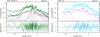 |
Fig. 3 EPIC spectra of region 1 (MOS1: black, MOS2: green, pn: cyan) and the background region (MOS1: red, MOS2: blue, pn: magenta) and the best-fit model. The thick solid lines show the source emission component (VNEI). The dotted lines show all the other components included in the model. |
3.1. Diffuse emission
To model the emission of the SNR, an additional thermal emission component was included for the source spectra. Best fit was achieved with a non-equilibrium ionisation model in both regions. We used the model VNEI which allowed us to vary the abundances. We used the solar element abundances determined by Anders & Grevesse (1989) for all fits. The best-fit parameter values are listed in Table 1.
The spectrum of region 1 is well fitted with a VNEI model assuming solar abundances (Fig. 3). If we also assume solar abundances for all elements for region 2, the fit is not sufficiently good and there are residuals especially at energies >1 keV. The fit improves if we free the abundances for Ne and Mg. The best fit indicates an overabundance of these two elements (see Table 1).
The X-ray emission from region 1 is consistent with emission from shocked ISM. This region 1 has a much higher surface brightness than the outer shock region to the east, which is seen in the radio map and is very faint in the X-rays (see the ROSAT contours in Fig. 1). The interior bright emission indicates that there was a region with higher density around the SN, i.e. circumstellar matter ejected from the progenitor. Inside this circumstellar matter, in region 2 we find enhanced abundances of selected elements (Ne, Mg), indicating emission from stellar ejecta.
3.2. Point-like sources
There are three bright hard sources clearly visible in Fig. 2, one of which coincides with the source CXO J192318.5+140305 suggested to be a PWN by Koo et al. (2005). The two hard sources at the northern rim of the FOV of the XMM-Newton observation correspond to the ASCA sources [KLS2002] HX3 east and west. We extracted and analysed the spectra of the diffuse emission in these regions.
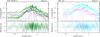 |
Fig. 4 EPIC spectra of region 2 (MOS1: black, MOS2: green, pn: cyan) and the background region (MOS1: red, MOS2: blue, pn: magenta) and the best-fit model, assuming two VNEI components for the source emission (see Sect. 4.1). The thick solid lines show the source emission component corresponding to shocked ISM (VNEI with solar abundances, parameters fixed to the results of region 1). The thick dash-dotted lines show the ejecta component. The dotted lines show all the other components included in the model. |
Fit parameters for the hard extended emission.
The source HX3 east has a counterpart in the radio (G49.2−0.3), which has been identified as a compact H ii region (Koo & Moon 1997a) and has thus been classified as emission from massive stars in G49.2−0.3. In the presented XMM-Newton data, the hard emission at the position of HX3 east has been resolved into two sources that are 17′′ apart (RA, Dec = 19 23 01.7, +14 16 34 and 19 23 01.8, +14 16 17) and have similar X-ray colours. We extracted the spectrum of a region that includes both sources. The spectrum was first fitted with a power-law model for the source emission. The background was modelled including the background components as described before. The resulting photon index is Γ = 3.2 (2.6−3.8)5 and the intrinsic absorption is NH = 3.5(3.0−4.9) × 1022 cm-2 (reduced χ2 = 1.4 for 299 degrees of freedom). A thermal emission model for a plasma in non-equilibrium ionisation instead of the non-thermal model improved the fit slightly (reduced χ2 = 1.3 for 297 degrees of freedom) and resulted in an intrinsic absorption of NH = 3.9(3.5−4.3) × 1022 cm-2, a temperature of kT = 2.4(1.8−3.5) keV, and an ionisation timescale of τ = 2.0(1.2−3.3) × 1010 s cm-3. The high photon index in the non-thermal fit is indicative of a thermal emission, whereas the high column density obtained in both fits suggests an emission origin embedded in a dense medium. The temperature and the ionisation timescale are also consistent with winds of young massive stars, confirming the results of Koo et al. (2002).
The source spectra of CXO J192318.5+140305 and HX3 west were modelled with a power-law component. The results are summarised in Table 2. Both sources are well fitted with a power-law spectrum with a photon index in the range of Γ = 1.7−2.0.
4. Discussion
4.1. Ejecta mass
The well-defined emission from region 2 allows us to estimate the amount of ejecta. To do so, we fitted the spectra of region 2 with a combined source model consisting of two VNEI models. For the first VNEI component, the parameters kT and τ were fixed to the best-fit values of region 1. The abundances were all set to solar. For the second VNEI spectrum, the parameters kT, τ, and the abundances of Ne and Mg were free, while all other abundances were set to zero first. In the subsequent steps we also fitted the abundances of all other elements by additionally freeing them one by one, but no other element showed a significantly enhanced abundance. This spectral component will allow us to estimate the amount of Ne and Mg in the ejecta. The spectra of region 2 with the best-fit model is shown in Fig. 4. As the best-fit parameters, we get the following values with lower 90% confidence limits for the normalisation of  cm-5, with D being the distance to the source, and the abundances for Ne = 180 (>10) and Mg = 50 (>20) × solar values. Since the fit parameters for the normalisation and the abundances are correlated to each other in this model, which is dominated by emission lines, it is not possible to constrain the upper confidence limits for these values.
At X-ray emitting temperatures, we can assume that all elements are almost fully ionised. In this case, we get ne = 1.21nH for the relation between the electron and H densities. The extraction region has an extent of about 10′. For the volume of the emitting region, we take the size of the extraction region and assume a depth of 10′, corresponding to the extent of the projected volume. For the calculations, we assume a distance of D = 6 kpc. We thus get a particle number density of nH = 0.07 (> 0.05) cm-3. For this density, we derive an ionisation time of τ/(1.21nH) = 3.0 × 10⁵ yr using the ionisation timescale obtained from the spectral fit of region 2. This time is one order of magnitude higher than the estimated age of the SNR (Koo et al. 1995, see Sect. 1). The ionisation timescale gives a characteristic number for the X-ray emitting plasma after it has been shocked and heated, and does not thus necessarily represent the real age of the SNR. As can be verified in Table 1, the ionisation timescale τ is significantly higher for region 2 than for the region 1, which is located outside region 2. This high ionisation age in the likely centre of the SNR surrounded by shocked circumstellar medium might indicate that the plasma is overionised, as observed in some mixed-morphology SNRs in our Galaxy (Lopez et al. 2013, and references therein).
Using the abundances obtained from the spectral fit, we estimate the masses of MNe = 2.9 (> 0.16) M⊙ and MMg = 0.30 (> 0.12) M⊙ for the ejecta. Because of the large uncertainties in determining the volume as well as the spectral fit parameters, these numbers only give a crude estimate of the masses. The comparison to calculated nucleosynthesis yields of SNe Type II by Nomoto et al. (1997) has shown that these mass limits for Ne and Mg point to a very massive progenitor with a mass of >20 M⊙.
4.2. Pulsar wind nebula candidates
The spectral analysis of the regions around CXO J192318.5+140305 and HX3 west have shown that both sources have a power-law spectrum with photon indices that are comparable and consitent with a PWN. The flux and the extent of the diffuse emission are also similar.
The hard source at the position of HX3 west consists of an extended emission and a hard point source, which is unfortunately located at the rim of the FOV. This makes a detailed analysis of the point source impossible. The three-colour Chandra image presented by Koo et al. (2005, their Fig. 1) also shows a blue (thus hard) point source at the north-western rim of the extended hard emission. As noted before, the hard sources at the positions of CXO J192318.5+140305 and HX3 west are very similar, both consisting of a diffuse emission plus a point source and the photon index of the extended emission being consistent with a PWN. The measured fluxes of the extended emission correspond to luminosities of L0.3−10.0 keV = 4.2(3.5−52.) × 1033 erg s-1 and 3.9(3.7−69.) × 1033 erg s-1 for CXO J192318.5+140305 and HX3 west, respectively, if we assume a distance of D = 6 kpc. At both positions, faint radio sources were found (Condon et al. 1998; Koo et al. 2002); therefore, we conclude that both sources are likely candidates of a PWN associated to the SNR W51C and require further investigation.
5. Summary
We have studied the Galactic SNR W51C using an observation of its central part carried out with XMM-Newton. It was not possible to analyse the X-ray emission of the outer blast wave as it was not covered completely by the pointing and the observed emission was too faint. However, the spectral analysis of the inner regions revealed that there are two distinct emission regions inside the SNR.
The first region has an arc-like morphology, more or less aligned to the morphology of the blast wave outside, but is much brighter. Its spectrum is well reproduced by thermal emission from plasma with non-equilibrium ionisation. The element abundances are consistent with solar values, indicating that the origin of this emission is shocked ambient medium. The shape and the higher X-ray brightness of this region suggest that the shocked material is the circumstellar medium of the progenitor.
The diffuse X-ray emission from the second region, located farther inside and in projection next to the region filled with colder gas and dust, is more highly absorbed and seems to arise from plasma close to collisional ionisation equilibium. Significantly enhanced abundances are measured for Ne and Mg. From the abundances and the density derived from the spectra, we calculated the masses of Ne and Mg in the ejecta and conclude that the progenitor was a massive star with a mass comparable to or higher than 20 M⊙.
In addition, we analysed the diffuse X-ray emission detected around two hard point sources, one of which has already been studied in detail by Koo et al. (2005) using Chandra data. The second hard source is located north-west of the region, close to the OH (1720 MHz) masers that have been found in W51C. The extended emission of both regions is well modelled with an absorbed power-law spectrum with a photon index of Γ ≈ 1.8. The luminosities are L0.3−10.0 keV ≈ 4 × 1033 erg s-1 for both regions;
the value is rather low, but still consistent with values measured for older PWNe (e.g., Kargaltsev & Pavlov 2010). In addition, the morphology of both sources consisting of a diffuse emission with an extent of ~1′ and a point source supports their classification as PWN candidates.
The XMM-Newton observation has enabled us to study the diffuse emission in the SNR W51C in detail and helped us to make a step forward in the classification of the underlying components of the complex X-ray emission of the SNR. Further observations will be necessary to study the blast wave of the SNR and to identify the possibly associated pulsar/PWN.
Acknowledgments
M.S. and G.W. acknowledge support by the Deutsche Forschungsgemeinschaft through the Emmy Noether Research Grant SA 2131/1-1. This research was funded through the BMWi/DLR grant 50 OR 1009. This research made use of data products from the Midcourse Space Experiment. Processing of the data was funded by the Ballistic Missile Defense Organization with additional support from NASA Office of Space Science. This research has also made use of the NASA/ IPAC Infrared Science Archive, which is operated by the Jet Propulsion Laboratory, California Institute of Technology, under contract with the National Aeronautics and Space Administration.
References
- Abdo, A. A., Ackermann, M., Ajello, M., et al. 2009, ApJ, 706, L1 [Google Scholar]
- Aleksić, J., Alvarez, E. A., Antonelli, L. A., et al. 2012, A&A, 541, A13 [Google Scholar]
- Anders, E., & Grevesse, N. 1989, Geochim. Cosmochim. Acta, 53, 197 [Google Scholar]
- Condon, J. J., Cotton, W. D., Greisen, E. W., et al. 1998, AJ, 115, 1693 [NASA ADS] [CrossRef] [Google Scholar]
- Copetti, M. V. F., & Schmidt, A. A. 1991, MNRAS, 250, 127 [NASA ADS] [Google Scholar]
- Egan, M. P., Price, S. D., Kraemer, K. E., et al. 2003, Air Force Research Laboratory Technical Report AFRL-VS-TR-2003-1589 [Google Scholar]
- Green, A. J., Frail, D. A., Goss, W. M., & Otrupcek, R. 1997, AJ, 114, 2058 [NASA ADS] [CrossRef] [Google Scholar]
- Hanabata, Y., Sawada, M., Katagiri, H., Bamba, A., & Fukazawa, Y. 2013, PASJ, 65, 42 [NASA ADS] [Google Scholar]
- Jansen, F., Lumb, D., Altieri, B., et al. 2001, A&A, 365, L1 [NASA ADS] [CrossRef] [EDP Sciences] [Google Scholar]
- Kargaltsev, O., & Pavlov, G. G. 2010, X-ray Astronomy 2009; Present Status, Multi-Wavelength Approach and Future Perspectives, AIP Conf. Ser., 1248, 25 [Google Scholar]
- Koo, B.-C., & Heiles, C. 1991, ApJ, 382, 204 [NASA ADS] [CrossRef] [Google Scholar]
- Koo, B.-C., & Moon, D.-S. 1997a, ApJ, 475, 194 [Google Scholar]
- Koo, B.-C., & Moon, D.-S. 1997b, ApJ, 485, 263 [Google Scholar]
- Koo, B.-C., Kim, K.-T., & Seward, F. D. 1995, ApJ, 447, 211 [Google Scholar]
- Koo, B.-C., Lee, J.-J., & Seward, F. D. 2002, AJ, 123, 1629 [Google Scholar]
- Koo, B.-C., Lee, J.-J., Seward, F. D., & Moon, D.-S. 2005, ApJ, 633, 946 [Google Scholar]
- Lopez, L. A., Pearson, S., Ramirez-Ruiz, E., et al. 2013, ApJ, 777, 145 [NASA ADS] [CrossRef] [Google Scholar]
- Mufson, S. L., & Liszt, H. S. 1979, ApJ, 232, 451 [NASA ADS] [CrossRef] [Google Scholar]
- Nomoto, K., Hashimoto, M., Tsujimoto, T., et al. 1997, Nucl. Phys. A, 616, 79 [NASA ADS] [CrossRef] [Google Scholar]
- Seward, F. D. 1990, ApJS, 73, 781 [NASA ADS] [CrossRef] [Google Scholar]
- Snowden, S. L., Collier, M. R., & Kuntz, K. D. 2004, ApJ, 610, 1182 [NASA ADS] [CrossRef] [Google Scholar]
- Snowden, S. L., Mushotzky, R. F., Kuntz, K. D., & Davis, D. S. 2008, A&A, 478, 615 [NASA ADS] [CrossRef] [EDP Sciences] [Google Scholar]
- Strüder, L., Briel, U., Dennerl, K., et al. 2001, A&A, 365, L18 [NASA ADS] [CrossRef] [EDP Sciences] [Google Scholar]
- Subrahmanyan, R., & Goss, W. M. 1995, MNRAS, 275, 755 [NASA ADS] [Google Scholar]
- Turner, M. J. L., Abbey, A., Arnaud, M., et al. 2001, A&A, 365, L27 [NASA ADS] [CrossRef] [EDP Sciences] [Google Scholar]
All Tables
All Figures
|
Fig. 1 A Midcourse Space Experiment (MSX, Egan et al. 2003) image in the infrared taken at 8.3 μm, together with ROSAT PSPC (0.1–2.4 keV) contours. The MSX image shows the emission from interstellar dust. The white cross marks the position of the OH (1720 MHz) masers. The white box indicates the field of the sky shown in Fig. 2. |
| In the text | |
|
Fig. 2 Three-colour image of the mosaic images (red: 0.3–1.0 keV, green: 1.0–2.0 keV, blue: 2.0–8.0 keV). Extraction regions used for the spectral analysis are shown. Point sources are removed. |
| In the text | |
|
Fig. 3 EPIC spectra of region 1 (MOS1: black, MOS2: green, pn: cyan) and the background region (MOS1: red, MOS2: blue, pn: magenta) and the best-fit model. The thick solid lines show the source emission component (VNEI). The dotted lines show all the other components included in the model. |
| In the text | |
|
Fig. 4 EPIC spectra of region 2 (MOS1: black, MOS2: green, pn: cyan) and the background region (MOS1: red, MOS2: blue, pn: magenta) and the best-fit model, assuming two VNEI components for the source emission (see Sect. 4.1). The thick solid lines show the source emission component corresponding to shocked ISM (VNEI with solar abundances, parameters fixed to the results of region 1). The thick dash-dotted lines show the ejecta component. The dotted lines show all the other components included in the model. |
| In the text | |
Current usage metrics show cumulative count of Article Views (full-text article views including HTML views, PDF and ePub downloads, according to the available data) and Abstracts Views on Vision4Press platform.
Data correspond to usage on the plateform after 2015. The current usage metrics is available 48-96 hours after online publication and is updated daily on week days.
Initial download of the metrics may take a while.