| Issue |
A&A
Volume 563, March 2014
|
|
|---|---|---|
| Article Number | A98 | |
| Number of page(s) | 13 | |
| Section | Planets and planetary systems | |
| DOI | https://doi.org/10.1051/0004-6361/201322702 | |
| Published online | 17 March 2014 | |
Thermophysical simulations of comet Hale-Bopp
Instituto de Astrofísica de Andalucía,
Glorieta de la Astronomía s/n 18008
Granada,
Spain
e-mail:
marta@iaa.es
Received:
18
September
2013
Accepted:
28
January
2014
Aims. In this work, we simulate the global behavior of comet Hale-Bopp with our thermophysical model starting with simple, homogeneous conditions, so that dust mantling and the active area develop consistently depending on the properties of the simulated nucleus. We aim to obtain a range of compatibility between our model and the observations, that can be used as constraints on some of the characteristics of cometary nuclei.
Methods. Our thermophysical model includes crystallization (and release of trapped CO), sublimation/recondensation, heat and gas transport through the nucleus, and dragged dust release. We run a battery of simulations with different parameter sets selected according to our current knowledge of comets and compare our results with observational data. Initial calculations are performed for a comet radius R0 = 30 km. To match the calculated integrated H2O production to the observed rate, we renormalize to a new R, which must be within 20 and 40 km, that is a range compatible with several estimates. Further selection is performed comparing the simulated water and carbon monoxide production rate profiles with the observational profiles and checking that the observational upper/lower limits of the H2O production are fulfilled.
Results. We have found a reasonable agreement between our model and the data for H2O and CO production rates, without the need of distributed sources, for the following initial conditions: the nucleus is composed of water, carbon monoxide, and dust with a moderate dust proportion, tending to be icy, with a dust-to-ice ratio of between 0.5 and 1. The water ice must be initially amorphous with 15 to 20% of trapped carbon monoxide. The icy matrix has a thermal inertia between 100 and 200 J m-2 K s−1/2, considering the initial composition with crystalline ice at 140 K. The dust follows an exponential size distribution with particles from 0.1 μm to 1 mm and leaves the comet dragged by the expelled vapor with a dragging efficiency (dust-to-gas ratio) of 3.
Key words: comets: general / comets: individual: Hale-Bopp / methods: numerical
© ESO, 2014
1. Introduction
Comet Hale-Bopp (C/1995 O1 Hale-Bopp) was discovered in 1995, and even at a heliocentric distance larger than 7 AU displayed a brightness of around 10 mags. Near perihelion, on April 1, 1997, Hale-Bopp was visible to the naked eye for more than a whole year, and even though post-perihelion activity was lower than preperihelion (see, e.g., Weaver et al. 1999), it continued for a long time. Szabó et al. (2008) detected activity at a distance of 25.7 AU from the Sun. This distant activity has been attributed to carbon monoxide, since temperatures that far from the Sun would be too low to produce water sublimation. In a later work, Szabó et al. (2011) made the furthest detection of Hale-Bopp, at 30.7 AU, proposing that it displayed some low level activity even that far from the Sun.
Although Hale-Bopp’s ephemerides show that 1997’s apparition was not its first passage through the inner Solar System (Marsden 1995), its dynamics indicate that it is a relatively young comet (see, e.g., Bailey et al. 1996). This work also revealed a change in the orbital parameters of Hale-Bopp due to a close encounter with Jupiter in April 1996.
The rotational state of comet Hale-Bopp is quite well determined: both Jorda et al. (1997) and Licandro et al. (1997) found a rotation period of approximately 11.34 h and also a similar rotation axis inclination. Their results are consistent with the estimates given by Vasundhara & Chakraborty (1999), who found a rotation axis inclination in the range [77°, 90°] with argument between 68° and 84°.
References for observational water, carbon monoxide, and dust production rates.
Apart from distant detection, the brightness of comet Hale-Bopp allowed an unprecedented study of its composition and production rates. We have compiled the production rates at different heliocentric distances for water, carbon monoxide, and dust provided by several authors and included these production rates in Table 1, which will be discussed later. Water and carbon monoxide production rates will be shown in many of the figures of the results section, such as Fig. 2, for comparison with our simulations. As for composition, all authors agree that carbon monoxide is the second most abundant volatile species, displaying a relatively high abundance relative to water. The mean abundance near perihelion is 24%, according to DiSanti et al. 2001, and 37 to 41%, according to Brooke et al. 2003. The slight agreement regarding a high carbon monoxide abundance in Hale-Bopp’s coma disappears when it comes to its source. DiSanti et al. (1999) and DiSanti et al. (2001) conclude that carbon monoxide production is fully nuclear at distances beyond 1.5 AU and that half of it comes from a distributed source at small solar distances. This is supported by Dello Russo et al. (2000) and Brooke et al. (2003) who suggest an extended source, probably carbonaceous particles, that would activate above a temperature threshold. On the other hand, Kuan et al. (2004) find that most of the carbon monoxide production of comet Hale-Bopp is consistent with nuclear production (in amounts comparable to those calculated by DiSanti et al. 2001).
The intense and persistent activity of comet Hale-Bopp and the associated brightness of its coma did not allow us to observe the nucleus clearly. This meant that, even though we have estimates of its effective size, the range covered by plausible radii is wide. Fernandez (2000) estimated the radius in 30 km, with an uncertainty of 10 km as a compatibility compromise with most of the observations, in a study similar to the one by Weaver & Lamy 1997. Estimates by Sekanina (1997), Altenhoff et al. (1999), and McCarthy et al. (2007) are within the range given by Fernandez (2000). Another consequence of this fact is that the geometry of the nucleus of Hale-Bopp is not constrained at all to the point where it has even been proposed that the nucleus is binary (Sekanina 1998).
1.1. Previous models
Since its discovery, Hale-Bopp has also been studied from the perspective of thermophysical models. Amongst them, we are going to focus on those developed by Enzian (1999), Kührt (1999, 2002), and Gortsas et al. (2011), since they are quasi-3D and so their results are most easily comparable with ours.
Enzian (1999) presented the evolution of a nucleus composed of amorphous ice, carbon monoxide, both trapped in the amorphous matrix and codeposited, and dust, with a dust-to-ice ratio of 1. Processes like erosion or dust mantling are not considered in this model, dust being a passive element that only affects the thermal properties of the icy matrix. The results obtained by Enzian (1999) show a reasonable fit for carbon monoxide production. However, to obtain those results they have to consider a rotation axis contained in the orbital plane after an orbit with a rotation axis perpendicular to the orbital plane. Moreover, the water production rate that they get is more than an order of magnitude lower than the observational data at large heliocentric distances.
Kührt (1999) considered a nucleus composed of crystalline ice and dust as a static component, with a model where the internal flux of gas or mantle formation are not considered. To fit the observations, they conclude that thermal conductivity must be low (0.001 W m-1 K-1) and emissivity close to unity. In a later work, Kührt (2002) reconsiders the problem with a more sophisticated model including carbon monoxide and internal gas flux. In those simulations, the thermal conductivity must be an order of magnitude higher to reproduce the water production rate. However, this thermal conductivity would not fit the data for carbon monoxide production, which would require an even higher conductivity. Recently, the work by Gortsas et al. (2011) simulates a nucleus composed by crystalline water ice, carbon monoxide ice, and dust, where the dust-to-ice ratio is 1, and 80% of volatile material corresponds to water ice. Gortsas et al. (2011) use a model where erosion is considered by means of solving a Stefan problem, but dust still acts as a static component in the matrix and the internal volatile flux is treated using a stationary approach. Even though they do not consider dust mantling, to match the observed productions, they use an active area fraction, which implies a surface quenching of the production given by the model; this area fraction is calculated a posteriori. The active area fraction can be justified by internal inhomogeneities or dust mantling, but neither of these processes is considered in the thermophysical model. In addition, water must come from the whole surface, with an active area fraction of 25%, whereas carbon monoxide must be produced in the northern hemisphere (latitudes below 10°) with an active area fraction of 75%.
1.2. Motivation
The amount of observational data available and the fact that, although not new, comet Hale-Bopp is not a very evolved object from the thermophysical standpoint make it an exceptional workbench for thermophysical models. The quasi 3D models that we have just described offer interpretations of the observed volatile productions, but we think that there is still room for improvement. On one hand, Enzian (1999) get a good agreement for carbon monoxide assuming amorphous ice with trapped carbon monoxide, but they fail to explain water production at large heliocentric distances. On the other hand, the model by Gortsas et al. (2011) needs a later adjustment of the active areas associated with each component to fit the observed production rates, but the processes that could make active areas appear are not modeled. Both models lack a dynamic treatment of the dust component and dust mantle formation, which is the main difference with the model presented here.
Our goal is to find an interpretation of the observed production rates of Hale-Bopp with our thermophysical model where the dust mantle (and thus, the active area fraction) will develop consistently with the hypothesis of the model, which will be described in the next section. We will start our simulations with initial homogeneous conditions, which represent the mean properties that can actually be deduced from observations. The nucleus will evolve according to its characteristics and the illumination conditions, so mantling can be developed inhomogeneously.
The capacity of our model to reproduce the data will indicate if it is possible to obtain an interpretation of Hale-Bopp’s nature, constraining some of its defining parameters, or if additional hypotheses like distributed production are necessary.
2. Method
2.1. Thermophysical model
We present a thermophysical model of heat and mass transfer through icy porous media applied to simulate the behavior of cometary nuclei. This model is an improvement of the one presented in González et al. (2008) used to study the evolution of the crystallization front in cometary conditions. Our model will consider heat and gas flux through the ice-dust matrix, sublimation and condensation of ices, dust drag and mantle formation, amorphous ice crystallization (and the associated release of energy and trapped gases), and erosion.
Given the uncertainty in the nucleus geometry, we have assumed that the nucleus of Hale-Bopp is spherical, although a great variability in the geometry of cometary nuclei has been found. The choice of a particular geometry has consequences for the calculated production rates (see, e.g., Gutiérrez et al. 2001). We have chosen a sphere because most parameters derived from observations (e.g., radius or density estimates) implicitly assume spherical geometry in their calculations.
The model is quasi-3D, which means that the surface is divided in facets, and at each one we will consider a one-dimensional approach in depth. Also, we will consider only a superficial layer in the nucleus. This will allow us to use plane-parallel geometry, which is an acceptable approach given that the superficial layer considered is small compared to the radius of the nucleus, and also enables the model to deal with geometrically irregular nuclei. We will also use a change of variables in depth so that the distance between nodes where the equations are solved follow an exponential distribution, the superficial ones being nearer than the inner ones (as done by, e.g., Tancredi et al. 1994).
Energetic and mass processes are coupled through the icy matrix, which allows for mass transfer through the pore system and solid state conduction, and also suffers transformations and phase changes with energetic consequences. All this is represented by a system of coupled partial differential equations (PDEs) describing mass and energy conservation in the cometary nucleus.
The mass equation for a volatile material α in the absence of additional sources is given by
the expression  (1)where
ρtotal,α represents
the density of material α through all its states and Jα represents the gas
flux. Given that the mean free path of molecules at the expected pressures in a cometary
context is larger than the assumed pore size, the flux can be assumed to be in Knudsen
regime, which allows us to treat the flux of each volatile component separately. The flux
of material α
is then expressed as (see, e.g., Prialnik 1992):
(1)where
ρtotal,α represents
the density of material α through all its states and Jα represents the gas
flux. Given that the mean free path of molecules at the expected pressures in a cometary
context is larger than the assumed pore size, the flux can be assumed to be in Knudsen
regime, which allows us to treat the flux of each volatile component separately. The flux
of material α
is then expressed as (see, e.g., Prialnik 1992):
 (2)where
Rg represents the ideal gas constant,
μα the molecular mass
of material α, L is the mean free path in the porous medium, and
the square root term represents the thermal velocity of the gas molecules.
(2)where
Rg represents the ideal gas constant,
μα the molecular mass
of material α, L is the mean free path in the porous medium, and
the square root term represents the thermal velocity of the gas molecules.
Water ice can be in amorphous, crystalline, or gas phase, represented by ρice,am, ρice,cr, and
ρvap,H2O,
respectively. In the context of cometary evolution, crystallization can be treated as an
irreversible process because amorphization due to solar radiation happens in very large
timescales compared to the orbital period, and other amorphization processes would require
pressures larger than those expected in comets (see, e.g., Huebner et al. 2006). Crystallization evolves at a rate that depends on
temperature. Since the temperatures at which crystallization is significant are lower than
those of water sublimation, we can also consider that all the water that actually
sublimates is crystalline. The amorphous ice equation can then be decoupled from the water
mass equation, obtaining:  (3)where
λ is the
temperature dependent crystallization rate, whose expression is given by Schmitt et al. (1989).
(3)where
λ is the
temperature dependent crystallization rate, whose expression is given by Schmitt et al. (1989).
The mass equation will be further decoupled through the sublimation/recondensation term
qα (see, e.g., Prialnik et al. 2004),  (4)where
ρα,sat is the
saturation density of material α, S is the specific surface, and ρα,vap its actual vapor
density.
(4)where
ρα,sat is the
saturation density of material α, S is the specific surface, and ρα,vap its actual vapor
density.
This way, vapor and ice densities can be calculated separately. In the case of water,
where we should also consider crystallization, for the crystalline ice we obtain:
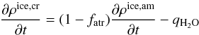 (5)where
fatr represents the fraction of carbon
monoxide trapped in the amorphous matrix.
(5)where
fatr represents the fraction of carbon
monoxide trapped in the amorphous matrix.
The water vapor equation expression is: 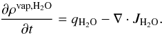 (6)For carbon monoxide,
following an analogous procedure and taking into account that it may be trapped in the
amorphous ice, we obtain:
(6)For carbon monoxide,
following an analogous procedure and taking into account that it may be trapped in the
amorphous ice, we obtain:  where
the last term represents the carbon monoxide released during crystallization.
where
the last term represents the carbon monoxide released during crystallization.
The thermal part of the model consists of the resolution of the energy conservation
equation, under the assumption that all the materials in the same location are at the same
temperature, that is, thermal equilibrium. Temperature is coupled to all of the above
mentioned densities (whose phase changes act as sources or sinks) as follows:
 (9)where
cα represents the
specific heat of each material, K represents the thermal conductivity of the icy
matrix, Hcrist is the net heat released during
crystallization, and Hα is the latent heat
of sublimation of species α. The left hand side of Eq. (9) is the variation in the internal energy of
the system. On the right, the first term is the energy transported by solid state
conduction and the second term is the energy released in crystallization. The third term
is the energy consumed (resp. released) in sublimation (resp. condensation) and the last
term is the energy transported by the gas flux.
(9)where
cα represents the
specific heat of each material, K represents the thermal conductivity of the icy
matrix, Hcrist is the net heat released during
crystallization, and Hα is the latent heat
of sublimation of species α. The left hand side of Eq. (9) is the variation in the internal energy of
the system. On the right, the first term is the energy transported by solid state
conduction and the second term is the energy released in crystallization. The third term
is the energy consumed (resp. released) in sublimation (resp. condensation) and the last
term is the energy transported by the gas flux.
Boundary conditions are required to solve the equations for temperature and each
material. In the interior of the nucleus the conditions are zero mass and energy flux, so
we have to choose an inner boundary deep enough so they can be fulfilled. At the surface,
the outward flux will be determined by the vapor going through the pores at the boundary
(Tancredi et al. 1994) as follows: 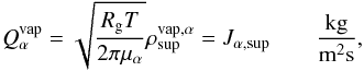 (10)where
 represents the amount of gas of material α in the pores at the surface.
The surface boundary condition for temperature will be an energy balance considering the
solar incoming flux, thermal reradiation, heat conduced to the interior and heat consumed
in sublimation (see, e.g., Huebner et al. 2006). In
the equation, 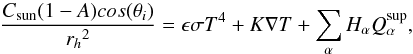 (11)Csun is the
solar constant, A represents the Bond albedo, θi the zenith angle of
the surface facet and rh is the
heliocentric distance. ϵ is the emissivity, σ the Stefan-Boltzmann
constant, K
is the thermal conductivity of the matrix and
(11)Csun is the
solar constant, A represents the Bond albedo, θi the zenith angle of
the surface facet and rh is the
heliocentric distance. ϵ is the emissivity, σ the Stefan-Boltzmann
constant, K
is the thermal conductivity of the matrix and  represents the amount of material α sublimating from the surface. Superficial
sublimation has an expression similar to that of
represents the amount of material α sublimating from the surface. Superficial
sublimation has an expression similar to that of  given in
Eq. (10), substituting the vapor density
for the saturation one and taking into account that only a fraction of the surface can
sublimate freely.
given in
Eq. (10), substituting the vapor density
for the saturation one and taking into account that only a fraction of the surface can
sublimate freely.
The total production rate of each volatile element α will be given by the sum
of the outward flux of α and the amount sublimated at the surface, where
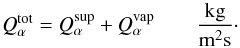 (12)Dust is dragged
by the gas flux, and it can leave the comet or form a superficial dust mantle. Only dust
smaller than a critical size will leave the comet (see, e.g., Huebner et al. 2006). The dust production rate will be proportional to
the total volatile production rate through an efficiency constant parameter
ef, which
models the dust to gas ratio in the coma, and provides us with the amount of dust dragged
by the gas leaving the comet, where
(12)Dust is dragged
by the gas flux, and it can leave the comet or form a superficial dust mantle. Only dust
smaller than a critical size will leave the comet (see, e.g., Huebner et al. 2006). The dust production rate will be proportional to
the total volatile production rate through an efficiency constant parameter
ef, which
models the dust to gas ratio in the coma, and provides us with the amount of dust dragged
by the gas leaving the comet, where 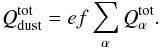 (13)Since it is necessary
that the dust is smaller than the critical radius r∗ to be
expelled, it is also important to consider a dust size distribution. For computational
reasons, we will consider a discretized version of a continuous distribution, so the total
amount of dust (represented by ρdust) will be distributed in
n
categories
(13)Since it is necessary
that the dust is smaller than the critical radius r∗ to be
expelled, it is also important to consider a dust size distribution. For computational
reasons, we will consider a discretized version of a continuous distribution, so the total
amount of dust (represented by ρdust) will be distributed in
n
categories  , each of
them characterized by a particle radius ri,i ∈ 1...n.
The distributions used for this work will be discussed further in the parameter section.
The total production of dust given in Eq. (13) will be divided amongst the dust categories with a radius smaller than the
critical radius, where
, each of
them characterized by a particle radius ri,i ∈ 1...n.
The distributions used for this work will be discussed further in the parameter section.
The total production of dust given in Eq. (13) will be divided amongst the dust categories with a radius smaller than the
critical radius, where 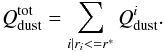 (14)For the dust flux, we
will make an assumption based on the one presented by Choi
et al. (2002), who supposed that the gas transport was so efficient that all the
vapor sublimated in the interior of the nucleus left it instantly. We will simplify the
dust flux so that all the dust that moves actually leaves the comet, and the dust residing
nearer the surface is expelled before the innermost dust. This way, once we calculate the
amount of dust of each category that must leave the comet is, we take it from the most
superficial volume elements that have dust of that size.
(14)For the dust flux, we
will make an assumption based on the one presented by Choi
et al. (2002), who supposed that the gas transport was so efficient that all the
vapor sublimated in the interior of the nucleus left it instantly. We will simplify the
dust flux so that all the dust that moves actually leaves the comet, and the dust residing
nearer the surface is expelled before the innermost dust. This way, once we calculate the
amount of dust of each category that must leave the comet is, we take it from the most
superficial volume elements that have dust of that size.
2.2. Observational data and the dust problem
As we have mentioned before, comet Hale-Bopp has been thoroughly observed by the scientific community, so there are a lot of observational data available. Amongst them, the most important for this work are the production rates presented in the references compiled in Table 1 for water, carbon monoxide, and dust.
Biver et al. (2002) calculated water (from OH) and carbon monoxide production from radio observations performed with several radio telescopes. Brooke et al. (2003) also provided water and carbon monoxide production from infrared spectroscopy obtained at the NASA Infrared Telescope Facility on Mauna Kea. Crovisier et al. (1999) obtained water and carbon monoxide production from spectroscopic observations with the Infrared Space Observatory (ISO). Woods et al. (2000) also got water (resp. carbon monoxide) production from OH (resp. C) measurements performed with the Solar Stellar Irradiance Comparison Experiment (SOLSTICE). Weaver et al. (1997, 1999) present results from data obtained with the Hubble Space Telescope. There, we can consult water production rates from molecular emission of OH in spectra as well as values of the Afρ parameter from absolute photometry. Dello Russo et al. (2000) used high-resolution infrared spectroscopy to obtain water production rates from direct observation of the water molecule.
Gunnarsson et al. (2003) present carbon monoxide production at large heliocentric distances from Swedish-ESO Submillimetre Telescope (SEST) spectra. They deduce a carbon monoxide production that is 40% lower than that of Biver et al. (2002) from the same data, since Gunnarsson et al. assume day/night differences, rather than isotropic production. DiSanti et al. (2001) estimated the carbon monoxide production rate from high-resolution infrared spectroscopy, also obtaining its rotational temperature and spatial coma distribution and deducing the existence of both a nuclear and a distributed source.
Combi (2000) revises the estimations for water production rate made by different authors and warns that given the large size of comet Hale-Bopp, the expansion velocities and kinetic temperatures reached in its coma (mostly around perihelion) may be larger than those usually assumed. This can lead to errors of a factor two in the production rates calculated. The effects addressed by Combi (2000) would lead to underestimations of the production rate, but as we have just seen, the underlying assumptions used to calculate production rates like the emission pattern can also lead to overestimations of almost a factor two. Usually formal errors are smaller than two but given the uncertainties in the emission pattern and the expansion velocities we will assume a conservative error estimate of a factor two, represented as the error bars shown in the figures of the next section. It is important to note that, although these error bars look symmetric in logarithmic scale plots (such as the majority of plots in this work), the length of the upper part of the error bars is twice the length of the lower part. The error bars in a linear scale look like those in Fig. 1.
Jewitt & Matthews (1999) presented dust observations in the submilimeter region, which is more sensitive to large particles than infrared or optical observations, with the James Clerk Maxwell Telescope on Mauna Kea. Rauer et al. (1997) calculated the Afρ parameter from optical observations with the Danish telescope at European Southern Observatory (ESO). Grün et al. (2001) performed infrared photometry with the ISO photo-polarimeter (ISOPHOT) and estimated the dust production rate on several dates.
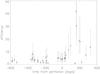 |
Fig. 1 Efficiency, calculated as Qdust/Qgas on the dates when there were dust data. The error bars show the factor 2 uncertainty in the gas production rate. |
Parameters explored in the whole set of simulations.
From all these data, given that water and carbon monoxide are by far the most abundant volatile species, we can estimate the dust dragging efficiency, calculated as the dust-to-gas production rate ratio Qdust/Qgas. Figure 1 shows the efficiency against time from perihelion. While volatile productions calculated by different authors are consistent and provide us with a coherent composite profile, dust production (and thus, efficiency, as plotted in Fig. 1) shows great dispersion and time variability. Part of this dispersion may be due to the different models and assumptions used to derive dust productions from observational data, and also to the inhomogeneity of the data (images in different wavelengths favor detection of dust grains in specific size ranges). In addition, variability and dispersion in Qdust/Qgas may mask effects and coma processes (e.g., dust fragmentation) with complex heliocentric dependencies. For these reasons, we will assume that efficiency is constant in time, although it will make it impossible to get volatile and dust productions simultaneously adjusted. We will thus only try to adjust both water and carbon monoxide production rates. Most of the preperihelion estimates are clustered around a mean value of 3, which is also within the error bars of the majority of Qdust/Qgas estimates.
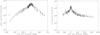 |
Fig. 2 Water (left) and carbon monoxide (right) production rates produced by the reference simulation, whose parameters are presented in Table 3. Black dots are the observational data given by the authors in Table 1; the error bars representing the conservative error estimate of a factor of 2 (see text). The gray dots with upper/lower arrows in the left panel represent upper/lower limits, respectively. |
2.3. Simulations and selection strategies
We have performed a battery of simulations of Hale-Bopp with orbitational and rotational parameters amongst the most accepted in the community, and combinations varying some of the magnitudes defining the nature of comet Hale-Bopp that are poorly constrained. The results presented here complete the previous work presented in González et al. (2012). The timespan simulated will be only one orbit, the one developed after a close encounter with Jupiter in 1996 (Bailey et al. 1996). This approach is justified since the previous semimajor axis was larger than 300 AU, which limited the activity to a small fraction of its orbital period. The results of multiorbit simulations by Capria et al. (2002) also support this approach. These simulations indicate that Hale-Bopp’s concentrated activity is associated with strong erosion, which would minimize the effects of thermophysical differentiation from previous orbits.
In Table 2, we have displayed the ranges of values over which we have varied the main parameters and initial conditions for the whole set of simulations. Since some of these parameters are coupled, not all combinations are acceptable, so we have chosen each simulation carefully to avoid inconsistencies. For example, variations in the dust-to-ice ratio change the relative amount of each component, which must be chosen so the specified bulk density is kept. This, in turn, will influence the thermal inertia, so we must also modify the hertz factor to keep the specified value for the thermal inertia. Another consequence of the coupling between magnitudes is the fact that modifications of the dust-to-ice ratio while keeping a constant bulk density will affect the porosity. To keep a specified value for the porosity, we would need to modify the bulk density.
As it can be seen in Table 2, the range we tried
is wide, sampling a significant part of the parameter space. The first parameter explored
is the dust to ice ratio, which will take values from 0.25 to 5 and test the production
rates of icy nuclei, dusty nuclei, and nuclei with a moderate percentage of ice. Also, the
relative abundance of mass of carbon monoxide (relative to that of water) is tested,
ranging from 0.1 to 0.2. This upper limit is larger than the classical ~15%, typically used for cometary ices. There is some uncertainty in
the conditions of formation of cometary ices, and recent works show dependence of the gas
trapping on the pressure of the gas (Yokochi et al.
2012), deposition temperature and rate, and even layer thickness (Bar-Nun et al. 2007). In any case, given all the
hypotheses used in the model, this amount of trapped carbon monoxide should be interpreted
as a very high concentration of carbon monoxide. One of the key magnitudes in this study
is the thermal inertia, which characterizes the global thermal behavior of the dust
matrix. Thermal inertia is given by  ,
where ρ,
K, and
c are the
global density, thermal conductivity, and specific heat of the matrix, respectively. The
strong coupling of thermal inertia to composition and conductivity (which evolve and have
complex dependencies) makes it difficult to compare the thermal inertia of different
simulations. This is why we will calculate the reference thermal inertia for each
simulation with the initial composition, assuming that the water ice is in crystalline
state and at a temperature of 140 K. We will control the thermal inertia (given a
composition) with the Hertz parameter, varying it accordingly from 4 × 10⁻⁴ to 0.125. We have also
explored the influence of the net energy released in crystallization, testing values
ranging from a purely exothermic crystallization, where the desorption of the trapped
dopant does not consume a large amount of energy, to an energetically neutral one, where
all the energy released during crystallization is consumed in the desorption of carbon
monoxide. Finally, we have tried several dust distributions, also presented in Table 2. All distributions consider five size categories
initially uniform in mass. This way, to define a dust distribution, we only need to
specify the radius of each category. Distribution 3 actually represents a monodisperse
distribution, but distributions 1 and 2 are discretized exponential distributions
n(r) = r−α
where α is
between 3 and 3.5, a range compatible with several fits of dust in the coma of Hale-Bopp
(see, e.g., Min et al. 2005; Lasue et al. 2009; Kolokolova et al.
2003). Dust Distribution 1 has an arbitrarily large last category (represented by
a particle radius of 1 m) so the formation of a dust mantle with this category of
undraggable dust is forced. Distribution 2 is the most realistic, with a wide radius
range, including several observational estimates of Hale-Bopp’s dust distribution (e.g.,
Lasue et al. 2009; Kolokolova et al. 2003), and also with a category representing
relatively large, but still draggable particles.
,
where ρ,
K, and
c are the
global density, thermal conductivity, and specific heat of the matrix, respectively. The
strong coupling of thermal inertia to composition and conductivity (which evolve and have
complex dependencies) makes it difficult to compare the thermal inertia of different
simulations. This is why we will calculate the reference thermal inertia for each
simulation with the initial composition, assuming that the water ice is in crystalline
state and at a temperature of 140 K. We will control the thermal inertia (given a
composition) with the Hertz parameter, varying it accordingly from 4 × 10⁻⁴ to 0.125. We have also
explored the influence of the net energy released in crystallization, testing values
ranging from a purely exothermic crystallization, where the desorption of the trapped
dopant does not consume a large amount of energy, to an energetically neutral one, where
all the energy released during crystallization is consumed in the desorption of carbon
monoxide. Finally, we have tried several dust distributions, also presented in Table 2. All distributions consider five size categories
initially uniform in mass. This way, to define a dust distribution, we only need to
specify the radius of each category. Distribution 3 actually represents a monodisperse
distribution, but distributions 1 and 2 are discretized exponential distributions
n(r) = r−α
where α is
between 3 and 3.5, a range compatible with several fits of dust in the coma of Hale-Bopp
(see, e.g., Min et al. 2005; Lasue et al. 2009; Kolokolova et al.
2003). Dust Distribution 1 has an arbitrarily large last category (represented by
a particle radius of 1 m) so the formation of a dust mantle with this category of
undraggable dust is forced. Distribution 2 is the most realistic, with a wide radius
range, including several observational estimates of Hale-Bopp’s dust distribution (e.g.,
Lasue et al. 2009; Kolokolova et al. 2003), and also with a category representing
relatively large, but still draggable particles.
As we have mentioned before, it is standard procedure in cometary modeling to fit production data to use an active area fraction as the factor that reduces the global production from the theoretical values to the observed ones. Since the active area fraction in our model will develop consistently with the model hypothesis and the initial conditions, we will proceed in a different way. Our simulations will be performed for a nucleus with a reference size radius Rnom= 30 km, the mean value estimated by Fernandez (2000). Once obtained a production for this reference size, we normalize the production obtained by our model so the integrated water production is the same as the integrated water production derived from the data taken from the references in Table 1. This way we get an effective radius R of the simulated nucleus of Hale-Bopp that will give us a criterion to evaluate our simulation. Only the simulations with effective radius R within the error considered in Fernandez (2000) are considered compatible. It is also important to note that we have checked through additional simulations that the a posteriori radius change does not introduce important profile differences with the normalized reference simulation.
Simulations whose effective radius was between 20 and 40 km have been visually inspected. We have tried to get a numerical criterion to compare our results with the data and estimate the quality of the fits (χ2 and reduced χ2 for the differences both in the production values and their logarithms for raw and smoothed results) and we found that its significance was poor. This was due to the fact that data cover values ranging several orders of magnitude. Since the quality of a fit is weighted by its magnitude, near perihelion values are more influential, minimizing the role of data taken at larger heliocentric distances. That is precisely where thermal diffusion is the dominant process and the inner part of the nucleus receives energy. To correct this behavior, we would need to introduce a weight system varying with heliocentric distance. This procedure, although mathematically elegant would condition our results favoring those that best reproduce the chosen weight. Thus, we have concluded that in this case a minimization technique associated with a numerical criterion would not offer better results than visual inspection.
3. Results
3.1. The reference simulation
We present the reference simulation, which is compatible with both observational water and carbon monoxide productions with an effective radius within the limits acceptable by Fernandez (2000). Fig. 2 shows the water and carbon monoxide production rates from the references in Table 1 with the error bars corresponding to a conservative error estimate of a factor of two, as previously explained. The lines in Fig. 2 represent the production rates calculated by our model for the dates on which we have observations, considering an effective radius of 23.85 km. Finally, the grey symbols with attached arrows in the water production plot represent the upper/lower limits for water production found in the references from Table 1.
The reference model overestimates water production at large heliocentric distances, and underestimates it around perihelion, resulting in a reasonable global adjustment. Nevertheless, considering the error bars, it is clear that our reference model reproduces reasonably well the behavior of water production at large heliocentric distances, fulfilling both upper and lower limits.
Carbon monoxide production is overestimated preperihelion, and presents large variations associated with the net energy released during crystallization. These are not noticeable in Fig. 2 because, both for the sake of clarity and because these are the only points of direct comparison, we only plot the model results when observations are available. The model and observational carbon monoxide production rates are compatible. Nevertheless, error bars leave some room for distributed sources, as will be discussed in a later section.
Parameters defining the reference simulation.
The rotation axis orientation causes seasonal variations of the production rates of the reference model. The Sun illuminates the southern hemisphere at large heliocentric distances, while the northern hemisphere receives sunlight only at perihelion. This causes the slope changes in the water production (see left panel of Fig. 2) and also that the dust mantle develops differently depending on the latitude. This is clear from Fig. 3, which will be discussed later in this section.
Table 3 shows the whole set of parameters that define the reference simulation. The whole set of simulations shares most of the parameters, and the reference case is characterized by those in boldface. The first section of Table 3 corresponds to the orbital and rotational parameters, and the former were taken from the Jet Propulsion Laboratory (JPL) small-body database. For the rotational parameters, as mentioned in the introduction of this work, the references are Jorda et al. (1997) and Vasundhara & Chakraborty (1999). Structural, compositional, and thermal parameters are amongst those typically used in cometary modeling. Those tagged with the superscript (a), resp (b), are from Huebner et al. (2006), resp. Tancredi et al. (1994). We have tried to choose simplified parameters due to the computational cost of simulations of the whole nucleus. For example, as done in Huebner et al. (2006), we have chosen the same constant value for the specific heat of ice and gas materials. This value has a bias toward the gas side, because in our model, the specific heat of solid components influences the results through thermal inertia, which can be controlled through other parameters, while the gas specific heat controls the heat transported through the vapor flux. The albedo and emissivity presented here are also widely used in cometary models (see, e.g., Enzian et al. 1997; Prialnik et al. 2004). The bulk density value listed in Table 3 is also standard, lying in the middle of the most favored range by different authors (see, e.g., Davidsson et al. 2007), 200−700 kg m-3. Additional simulations with bulk densities of 300 and 700 kg m-3 did not show significant variations in the overall production rate profiles.
It may be possible to obtain a better fit with parameters near those of the reference model (listed in Table 3), but it would not make sense since we are looking for a qualitative agreement, starting with average (although realistic) initial properties of the nucleus and not considering effects like nucleus elongation or inhomogeneities. In the next section, we will use the reference model as a basis and vary some of the parameters listed in Table 2 to obtain a range of compatibility of our model and the observations.
Given that both water and carbon monoxide production rates are reasonably fitted by the reference model, the carbon monoxide abundance ratio (as the factor QCO/QH2O) from the reference simulation is also similar to the one based on observational data, as expected. The values of this observational abundance cover almost two orders of magnitude, confirming that coma volatile abundances do not represent those in the nucleus.
The reference simulation is characterized by a moderate dust mantle development, driven by volatile production. This is due to a dust size distribution with a large range of particle sizes (Distribution 2 in Table 2, with particle radii ranging from 10-7 to 10-3 m) and a dragging efficiency of 3, relatively large but compatible with the average efficiency calculated from the observational data (displayed in Fig. 1). As the simulated nucleus moves along its orbit, the surface erodes and a dust mantle is developed. The evolution of erosion and mantling will present differences according to the illumination conditions in each zone of the surface. Once dust is settled on the surface, erosion drastically reduces, although there still may be significant production.
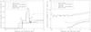 |
Fig. 3 Left: Longitudinally averaged mantle thickness of the reference simulation case against distance from perihelion for five latitudinal bands. Right: Analogous plot of longitudinally averaged carbon monoxide front depth. In these plots, negative distances represent values pre-perihelion. |
In the left plot of Fig. 3, we can see the latitude-averaged mantle thickness against distance to perihelion. The dust mantle tends to be thicker as we approach the north pole, except in the north pole itself, where postperihelion recondensation is significant and reduces the mantle from 37 to 16 cm. Recondensation takes place at all latitudes after the growth of the mantle once illumination stops. The seasonal differences in illumination are the cause of the differences in the growth velocities at different latitudes.
The crystallization front and the carbon monoxide sublimation front are located at greater depth in the southern hemisphere than in the northern. Proof of this can be seen in the right plot of Fig. 3, where the latitude-averaged depth of the carbon monoxide is shown. This is because erosion and water sublimation (responsible for mantling) are superficial phenomena, while crystallization and carbon monoxide sublimation happen at a certain depth. Volume processes are favored by a weaker, but longer energy input, as happens in the southern hemisphere, since a greater proportion of the energy received is then conducted to the interior. The same reason accounts for the different location of the sources of water and carbon monoxide production. While water is produced in the illuminated zones where the dust mantle is thin, carbon monoxide production is generally not localized, since it comes from the crystallization front and the carbon monoxide sublimation front, both in the nucleus interior.
3.2. Variation of parameters
When we considered the whole set of simulations, it became clear that the development of a dust mantle is the key factor in the production rate profiles obtained in our simulations. Although this process is dependent on several of the parameters that we vary in our simulations, we can distinguish two large groups of simulations that are not compatible with the observational data and are associated with excess or absence of a dust mantle. In this section we will see examples of both of these situations, and also others that can arise when exploring the parameter space.
3.2.1. Dust distribution and dragging efficiency
Since the role of dust mantling in the evolution of cometary nuclei is essential, we start the parameter space exploration with two magnitudes that directly modify the ability of the system to develop a dust mantle: dust size distribution and dragging efficiency.
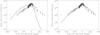 |
Fig. 4 Left: Water production rate against time of a nucleus where the dust dragging efficiency is reduced from the reference value to 1. This represents the behavior of water production rates when dust mantle is forced. Right: Water production rate against time of a nucleus with a monodisperse distribution of small particles (Distribution 3 in Table 2), which represents the behavior of water production rates when there is no dust mantling. In both cases, the rest of parameters are the same as those presented in Table 3. |
When there is dust so large that it can not be dragged or the efficiency is too small to allow the gas flux to drag a significant amount of dust, mantle formation is forced and we obtain similar profiles. As an example, we can see on the left panel of Fig. 4 the water production rate profile in the case of a simulation where efficiency has been reduced from the reference value of 3 to 1. In addition to the poor fit of the profile, in this case productions are so quenched that the effective radius previously defined is 48.5 km. The case of the Distribution 1 in table 2 (which had a category of dust too large to be dragged) is analogous to the case we have just described, with a production rate very similar to the one shown in the left panel of Fig. 4 and an effective radius of 60.85 km.
The opposite case occurs when dust mantle is not formed. Then, compatibility of the data with observations requires the effective radius to be much smaller than what is currently accepted. In the right panel of Fig. 4, the water production for a simulation with a monodisperse dust size distribution with radius 1 μm and the rest of parameter set to the reference values is displayed. This corresponds to Distribution 3 in Table 2, for which the dust is easily dragged by the gas flux and thus hinders dust mantle formation. Since the production of a nucleus where water sublimates directly from the surface is large, in this case the effective radius of the nucleus is 15.2 km. This result is very similar to the results obtained by Gortsas et al. (2011) and Kührt (2002), and is expected since they do not consider dust mantle formation, so water sublimates freely from the nucleus surface. Moreover, the carbon monoxide production rate of this simulation does not reproduce the observations, and is systematically and substantially below the error bars.
3.2.2. Thermal inertia
The increase of thermal inertia from the reference value to 500 W K-1 m-2 s−1/21 leads us to a similar situation to the one we have just described. The global profile for water production is reasonable, although it decreases too fast postperihelion. Nevertheless, the effective radius is 14.52, much less than the accepted estimations. The dust mantle does not develop because higher thermal inertia makes mean crystallization velocity higher (González et al. 2008), so a large amount of carbon monoxide is released, dragging a large amount of dust grains and also large dust grains.
 |
Fig. 5 Water production rate for a nucleus with a thermal inertia of 50 W K-1 m-2 s−1/2, reduced compared to that of the reference model. The rest of parameters defining this simulation are the same as the reference model and can be consulted in Table 3. |
The behavior of simulations with a reduced thermal inertia (50 W K-1 m-2 s−1/2) is more complex. The mean crystallization rate is lower, which favors mantle development. The mantle formed in this simulation is a better thermal insulator since, as we have mentioned before, thermal inertia is changed through the Hertz factor. This means that the thermal conductivity of the simulation with reduced thermal inertia is lower than in the reference case, so the zone under a dust mantle of a fixed thickness receives less energy. This causes the dust mantle development to stop earlier, so the final mantle is thinner than the one in the reference simulation. Fig. 5 shows the water production rate in the case of a simulation with I = 50 W K-1 m-2 s−1/2 and the remaining parameters as those in Table 2. The effective radius for this simulation is within the acceptable range ( 32.05 km), but the water profile slope is much lower than the observation, particularly postperihelion. In addition, the upper limit postperihelion is not fulfilled, so we consider that the water production is not well reproduced with this simulation. Additional simulations with intermediate values for thermal inertia (100 W K-1 m-2 s−1/2) give better results, though still worse than those from the reference model.
3.2.3. Dust-to-ice ratio
Dust-to-ice ratio is a magnitude coupled with all the rest affecting the system evolution. The net quantities of dust and ice are modified, and this has consequences both on the thermal properties and the production.
First, we describe the results of using a large dust-to-ice ratio, of 5. The water profile is very similar to those at the beginning of this section, where the dust mantle was forced using an efficiency of 1 (left panel in Fig. 4). Water production is low, and the effective radius increases to 68.9 km. The main difference is that dust mantle is much thicker in this case, of the order of tenths of meters.
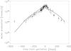 |
Fig. 6 Water production rate for a nucleus with a reduced dust-to-ice ratio of 0.5. The rest of parameters defining this simulation are the same as the reference model and can be consulted in Table 3. |
In Fig. 6, the results of the simulation where the dust-to-ice ratio is diminished to 0.5 can be seen. Global water ice production looks acceptable although the water production obtained with this model is actually excessive, since the effective radius is 17.84 km. This is due to the absence of a dust mantle in the southern hemisphere. The water production peak appears before the observational one due to the rapid formation of an insulating dust mantle during perihelion.
3.2.4. Amount of carbon monoxide
 |
Fig. 7 Water (left) and carbon monoxide production rates produced by a simulation with 15% in mass of trapped carbon monoxide. The rest of parameters are the same as those presented in Table 3. |
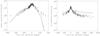 |
Fig. 8 Left: Water production rate for a nucleus composed of crystalline ice where carbon monoxide is codeposited. The rest of the parameters defining this simulation are the same as the reference model and can be consulted in Table 3. Right: Carbon monoxide production rate for the same simulation. |
Figure 7 shows the water and carbon monoxide production rates for a nucleus in which carbon monoxide trapped in the amorphous ice is 15% of the latter (in mass). The agreement between the simulated and the observed water production is excellent, perhaps even better than the reference simulation and the effective radius is 20.25 km, right in the lower limit of the accepted estimates. Nevertheless, this simulation produces less carbon monoxide (see right panel of Fig. 7) than the reference simulation, and the carbon monoxide production is systematically below the error bars. This is why we favor the global results from the eference simulation. In any case, these differences might be compensated with distributed production if a significant amount of source material was expelled postperihelion or if we consider initial inhomogeneities of the nucleus, but that is beyond the scope of this work.
3.2.5. Phase of water ice and energy released in crystallization
We have verified our main hypotheses, namely that the nucleus is initially formed by amorphous water ice hosting carbon monoxide. We present a simulation where all the water ice is in the crystalline phase with carbon monoxide codeposited as ice. The left plot of Fig. 8 shows that the model water production is quite similar to the observational data in the preperihelion branch, but postperihelion the former drops too fast.
Carbon monoxide production presents a profile that is too flat to fit the observational data, as can be seen in the right panel of Fig. 8. Even though the magnitude of carbon monoxide production is suitable, it does not descend as the data indicate it should. The cause is that there is not a thick layer of insulating amorphous ice above the carbon monoxide sublimation front, since the water ice is initially crystalline. Additional simulations indicate that simulations with amorphous ice and initially condensed carbon monoxide (instead of trapped) display a similar behavior. In these simulations, although the carbon monoxide sublimation front was always in the amorphous zone, it was located deeper in the case of initially trapped carbon monoxide, since recondensation of the liberated carbon monoxide was needed for the formation of a sublimation front. This caused the insulating amorphous layer to be significantly thicker for the case where carbon monoxide was trapped.
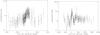 |
Fig. 9 Observed production rate to reference simulation production rate ratio Qobs/Qmod for water (left) and carbon monoxide (right). The error bars account for a factor 2 error, as described in the text. |
In additional simulations, the effect of the energy consumed by the volatile trapped in the amorphous matrix (which effectively reduces the net energy released in crystallization) has been tested. When the net energy released in crystallization is halved, on the one hand the water production rate is similar to the case with crystalline ice, which is too steep post perihelion. This is because the amount of energy stored near the surface is not enough to sustain water sublimation. On the other hand, carbon monoxide is systematically higher than the observations obtained preperihelion and stays in the upper limit of the error bars during the postperihelion branch of the orbit. A lower amount of trapped carbon monoxide could diminish the carbon monoxide discrepancies, but not the water production rate discrepancies. We have also performed simulations considering that trapped carbon monoxide desorption consumes an amount of energy equal to its latent heat of sublimation weighted by its abundance during crystallization (see, e.g., Prialnik et al. 2004). These results do not vary significantly from the reference case, since the final amount of energy consumed in desorption with this parametrization is small. Considering those simulations, we, therefore, conclude that the energy released during crystallization must be greater than 4.5 × 10⁴ J kg -1 to be compatible with the observations of comet Hale-Bopp.
4. Discussion
The complete set of simulations that we have just described shows that it is possible to offer an interpretation of the behavior of comet Hale-Bopp using the assumptions of our model.
The water and carbon monoxide production rates obtained with the reference simulation are compatible with the observations, considering a conservative error estimate. The rest of the simulations presented here explore the parameter space to show the limits where the simulated production rates stop being compatible with the observational rates.
4.1. Distributed sources
The possible presence of distributed sources for the water and carbon monoxide production is still a source of disagreement amongst the scientific community, as we have seen previously. Since distributed sources are not a hypothesis in our model, we will analyze the likelihood of this assumption in the context of the reference simulation.
Figure 9 shows the ratio of the observed production rate and the production rate Qobs/Qmod modeled with the reference model, both for water (left) and carbon monoxide (right). Although this representation magnifies the differences between the observed and the modeled production, considering the error bars, the results of the reference model are still compatible with the observations most of the time. However, tendencies are better studied considering just the observational data, represented in Fig. 9 as dots. As already explained, the water production rate (left plot of Fig. 9) shows a reasonable global agreement with the observations, despite some underestimation around perihelion and overestimation in the preperihelion branch of the orbit. If the hypotheses used in the reference model are correct, distributed sources as the expulsion of water ice grains would be compatible with the observations around perihelion and in a relatively small amount. In that case, as indicated by Gunnarsson et al. (2003), the icy grains would sublimate so quickly that its production would be impossible to distinguish from nuclear emission.
Even though the reference simulation results are compatible with the observations, carbon monoxide production could be underestimated by the model, since production rates 1.5 or 2 times higher than the model would still be compatible with the observations. The median of Qobs/Qmod is 1.57, which implies that, on average, around a third of the total observed carbon monoxide could have a distributed source origin. The expulsion of icy grains is not a plausible possibility of distributed production, since the carbon monoxide ice is quite far from the surface (see Fig. 3). In addition, as we have just explained, if water ice grains (which are nearer the surface) were expelled it would be in a small amount, which makes carbon monoxide ice expulsion even less plausible. The most promising hypotheses for a carbon monoxide distributed source would be the dust, which could produce carbon monoxide above a thermal threshold.
In any case, both for the case of water and carbon monoxide, the uncertainty in the nucleus size does not allow us to draw definite conclusions about the presence of distributed sources. We can only say that the reference model would be compatible with ~1/3 of the total carbon monoxide production coming from a distributed source, particularly in the post-perihelion branch of the orbit. This amount, however, would be of the order of the error estimates we have used, so we cannot categorically state it.
4.2. Amorphous ice
The possibility of the cometary ice being amorphous is still an open problem within the cometary community. Our simulations strongly suggest that the water ice in the nucleus of comet Hale-Bopp was initially amorphous. In the first place, the carbon monoxide profile would be much flatter if we considered the water ice crystalline and carbon monoxide codeposited (see Fig. 8). Moreover, for a simulation like the reference but with crystalline ice, the water production rate profile presented a slope that was too steep in the postperihelion region of the orbit. This same effect in the water ice production also happened when we considered a simulation where the energy released in crystallization of the amorphous ice was halved compared to that of the reference simulation. This indicates that the postperihelion water activity is partly sustained by the accumulation of crystallization energy in the zone between the surface and the crystallization front.
The presence of amorphous water ice in comet Hale-Bopp has cosmogonic consequences. The work Prialnik et al. (1987) models the consequences of radiogenic heating of comet nuclei during early evolution in the transneptunian reservoirs. Their results are that the heat released during 26Al decay would crystallize cometary material almost completely. This way, for the preservation of amorphous ice cometary nuclei should have been formed 4-5 million years after condrite condrules. Our model favors amorphous presence in comets and, thus, this scenario.
5. Conclusions
We have simulated simultaneously the behavior of water and carbon monoxide productions determined by observations of comet Hale-Bopp, and obtained an interpretation of the nature of the comet nucleus using our thermophysical model. The magnitudes that define our reference model, representing the behavior of comet Hale-Bopp, are described in Table 3. We have to note that, given the coupling of the magnitudes involved, other similar sets of parameters can also give good results. The values listed in Table 3 must be considered an approximation to the nucleus characteristics. From the sensitivity study to variations in the main parameters, we can conclude that our model reproduces the behavior displayed by comet Hale-Bopp when:
-
The nucleus is initially composed of dust and amorphous ice containing carbon monoxide trapped within its structure.
-
Thermal inertia is moderate, of the order of 200 W m-2 K-1 s−1/2, being acceptable values from 100 W m-2 K-1 s−1/2. This value is around the upper limit considered for cometary material, but it is important to note that this is only a reference value to allow for the comparison of different simulations considering crystalline ice at 140 K. The actual value of thermal inertia in our model depends on the particular composition and temperature at each location and time.
-
Dust-to-ice ratio is moderate to low, between 0.5 and 1, indicating a balanced nucleus tending to be icy.
-
The amount of carbon monoxide is between 15% and 20% of the mass of amorphous ice (which is 7.5 to 10% of the total mass, assuming a dust to ice ratio of 1). The carbon monoxide must be initially trapped in the amorphous ice and it can condense in colder regions of the nucleus after being released during crystallization.
-
The net energy released in crystallization is high. This implies that, according to our results, the energy invested in the liberation of the trapped carbon monoxide must be very low compared to that released during crystallization.
These characteristics by themselves do not reproduce the behavior of the comet, since we have proved that dust mantling plays a key role in comet nuclei evolution. Hale-Bopp’s production rates can be explained if a dust mantle is produced in almost the whole surface, hindering water production. Our simulations favor a dust size distribution like Distribution 2 in Table 2, relatively ample and also globally compatible with observational data.
The presence of amorphous water ice in comet Hale-Bopp has cosmogonic consequences. The model of early cometary thermal evolution by Prialnik et al. (1987) indicates that for the conservation of amorphous ice cometary nuclei should have been formed 4-5 million years after condrite condrules. Our model favors amorphous presence in comets and, thus, this scenario.
As for the presence of distributed sources, we can only say that the reference model, being compatible by itself with the observations, would also be compatible with ~1/3 of the total carbon monoxide production coming from a distributed source. Given the order of the error estimates we have used and the uncertainty in the nucleus size, we cannot draw a definite conclusion on this subject.
Finally, we should mention that the dust production behavior could not be simulated along with gas production, although the best results point to an efficiency of 3, similar to the mean value of the observational efficiency (see Fig. 1). Observations indicate that the relationship between gas and dust expelled is highly variable. If this is correct (and not due to the observational response of any process in the coma), it may indicate that either the dust dragging process has some dependencies that we still ignore or that there is another process involved in expelling dust that has not been taken into account. This obvious limitation is also an interesting problem for future study.
Acknowledgments
While doing this research, M. González was hired by the Spanish National Research Council (Consejo Superior de investigaciones científicas-CSIC), program JAE-Pre, partly funded by the European Science Foundation (ESF).
References
- Altenhoff, W. J., Bieging, J. H., Butler, B., et al. 1999, A&A, 348, 1020 [NASA ADS] [Google Scholar]
- Bailey, M. E., Emel’Yanenko, V. V., Hahn, G., et al. 1996, MNRAS, 281, 916 [NASA ADS] [CrossRef] [Google Scholar]
- Bar-Nun, A., Notesco, G., & Owen, T. 2007, Icarus, 190, 655 [NASA ADS] [CrossRef] [Google Scholar]
- Biver, N., Bockelée-Morvan, D., Colom, P., et al. 2002, Earth Moon Planets, 90, 5 [NASA ADS] [CrossRef] [Google Scholar]
- Brooke, T. Y., Weaver, H. A., Chin, G., et al. 2003, Icarus, 166, 167 [NASA ADS] [CrossRef] [Google Scholar]
- Capria, M. T., Coradini, A., & de Sanctis, M. C. 2002, Earth Moon Planets, 90, 217 [NASA ADS] [CrossRef] [Google Scholar]
- Choi, Y.-J., Cohen, M., Merk, R., & Prialnik, D. 2002, Icarus, 160, 300 [NASA ADS] [CrossRef] [Google Scholar]
- Colom, P., Gérard, E., Crovisier, J., et al. 1997, Earth Moon Planets, 78, 37 [Google Scholar]
- Combi, M. 2000, Earth Moon Planets, 89, 73 [NASA ADS] [CrossRef] [Google Scholar]
- Crovisier, J., Leech, K., Bockelée-Morvan, D., et al. 1999, in The Universe as Seen by ISO, eds. P. Cox, & M. Kessler, ESA SP, 427, 137 [Google Scholar]
- Davidsson, B. J. R., Gutiérrez, P. J., & Rickman, H. 2007, Icarus, 187, 306 [NASA ADS] [CrossRef] [Google Scholar]
- Dello Russo, N., Mumma, M. J., DiSanti, M. A., et al. 2000, Icarus, 143, 324 [NASA ADS] [CrossRef] [Google Scholar]
- DiSanti, M. A., Mumma, M. J., Dello Russo, N., et al. 1999, Nature, 399, 662 [NASA ADS] [CrossRef] [Google Scholar]
- DiSanti, M. A., Mumma, M. J., Dello Russo, N., & Magee-Sauer, K. 2001, Icarus, 153, 361 [NASA ADS] [CrossRef] [Google Scholar]
- Enzian, A. 1999, Space Sci. Rev., 90, 131 [NASA ADS] [CrossRef] [Google Scholar]
- Enzian, A., Cabot, H., & Klinger, J. 1997, A&A, 319, 995 [NASA ADS] [Google Scholar]
- Fernandez, Y. 2000, Earth Moon Planets, 89, 3 [Google Scholar]
- González, M., Gutiérrez, P. J., Lara, L. M., & Rodrigo, R. 2008, A&A, 486, 331 [NASA ADS] [CrossRef] [EDP Sciences] [Google Scholar]
- González, M., Gutiérrez, P. J., & Lara, L. M. 2012, LPI Contrib., 1667, 6167 [NASA ADS] [Google Scholar]
- Gortsas, N., Kührt, E., Motschmann, U., & Keller, H. U. 2011, Icarus, 212, 858 [NASA ADS] [CrossRef] [Google Scholar]
- Grün, E., Hanner, M. S., Peschke, S. B., et al. 2001, A&A, 377, 1098 [NASA ADS] [CrossRef] [EDP Sciences] [Google Scholar]
- Gunnarsson, M., Bockelée-Morvan, D., Winnberg, A., et al. 2003, A&A, 402, 383 [NASA ADS] [CrossRef] [EDP Sciences] [Google Scholar]
- Gutiérrez, P. J., Ortiz, J. L., Rodrigo, R., & López-Moreno, J. J. 2001, A&A, 374, 326 [NASA ADS] [CrossRef] [EDP Sciences] [Google Scholar]
- Huebner, W. F., Benkhoff, J., Capria, M.-T., et al. 2006, Heat and Gas Diffusion in Comet Nuclei (Noordwijk: ESA Publications Division) [Google Scholar]
- Jewitt, D., & Matthews, H. 1999, AJ, 117, 1056 [NASA ADS] [CrossRef] [Google Scholar]
- Jorda, L., Rembor, K., Lecacheux, J., et al. 1997, Earth Moon Planets, 77, 167 [Google Scholar]
- Kolokolova, L., Lara, L., Schultz, R., Stuewe, J., & Tozzi, G.-P. 2003, J. Quant. Spectr. Rad. Transf., 79, 861 [NASA ADS] [CrossRef] [Google Scholar]
- Kuan, Y.-J., Pen, M.-L., Huang, H.-C., Veal, J. M., & Woodney, L. M. 2004, in Bioastronomy 2002: Life Among the Stars, eds. R. Norris, & F. Stootman, IAU Symp., 213,189 [Google Scholar]
- Kührt, E. 1999, Space Sci. Rev., 90, 75 [NASA ADS] [CrossRef] [Google Scholar]
- Kührt, E. 2002, Earth Moon Planets, 90, 61 [NASA ADS] [CrossRef] [Google Scholar]
- Lasue, J., Levasseur-Regourd, A. C., Hadamcik, E., & Alcouffe, G. 2009, Icarus, 199, 129 [NASA ADS] [CrossRef] [Google Scholar]
- Licandro, J., Bellot Rubio, L. R., Casas, R., et al. 1997, Earth Moon Planets, 77, 199 [Google Scholar]
- Marsden, B. G. 1995, IAU Circ., 6224 [Google Scholar]
- McCarthy, D. W., Stolovy, S. R., Campins, H., et al. 2007, Icarus, 189, 184 [NASA ADS] [CrossRef] [Google Scholar]
- Min, M., Hovenier, J. W., de Koter, A., Waters, L. B. F. M., & Dominik, C. 2005, Icarus, 179, 158 [NASA ADS] [CrossRef] [Google Scholar]
- Prialnik, D. 1992, ApJ, 388, 196 [NASA ADS] [CrossRef] [Google Scholar]
- Prialnik, D., Bar-Nun, A., & Podolak, M. 1987, ApJ, 319, 993 [NASA ADS] [CrossRef] [Google Scholar]
- Prialnik, D., Benkhoff, J., & Podolak, M. 2004, in Comets II, eds. M. C. Festou, H. U. Keller, & H. A. Weaver, 359 [Google Scholar]
- Rauer, H., Arpigny, C., Boehnhardt, H., et al. 1997, Science, 275, 1909 [NASA ADS] [CrossRef] [Google Scholar]
- Schmitt, B., Espinasse, S., Grim, R. J. A., Greenberg, J. M., & Klinger, J. 1989, in Physics and Mechanics of Cometary Materials, eds. J. J. Hunt, & T. D. Guyenne, ESA SP, 302, 65 [Google Scholar]
- Sekanina, Z. 1997, Earth Moon Planets, 77, 147 [Google Scholar]
- Sekanina, Z. 1998, ApJ, 509, L133 [NASA ADS] [CrossRef] [Google Scholar]
- Szabó, G. M., Kiss, L. L., & Sárneczky, K. 2008, ApJ, 677, L121 [NASA ADS] [CrossRef] [Google Scholar]
- Szabó, G. M., Sárneczky, K., & Kiss, L. L. 2011, A&A, 531, A11 [NASA ADS] [CrossRef] [EDP Sciences] [Google Scholar]
- Tancredi, G., Rickman, H., & Greenberg, J. M. 1994, A&A, 286, 659 [NASA ADS] [Google Scholar]
- Vasundhara, R., & Chakraborty, P. 1999, Icarus, 140, 221 [NASA ADS] [CrossRef] [Google Scholar]
- Weaver, H. A., & Lamy, P. L. 1997, Earth Moon Planets, 79, 17 [Google Scholar]
- Weaver, H. A., Feldman, P. D., A’Hearn, M. F., & Arpigny, C. 1997, Science, 275, 1900 [NASA ADS] [CrossRef] [PubMed] [Google Scholar]
- Weaver, H. A., Feldman, P. D., A’Hearn, M. F., et al. 1999, Icarus, 141, 1 [NASA ADS] [CrossRef] [Google Scholar]
- Woods, T. N., Feldman, P. D., & Rottman, G. J. 2000, Icarus, 144, 182 [NASA ADS] [CrossRef] [Google Scholar]
- Yokochi, R., Marboeuf, U., Quirico, E., & Schmitt, B. 2012, Icarus, 218, 760 [NASA ADS] [CrossRef] [Google Scholar]
All Tables
All Figures
|
Fig. 1 Efficiency, calculated as Qdust/Qgas on the dates when there were dust data. The error bars show the factor 2 uncertainty in the gas production rate. |
| In the text | |
|
Fig. 2 Water (left) and carbon monoxide (right) production rates produced by the reference simulation, whose parameters are presented in Table 3. Black dots are the observational data given by the authors in Table 1; the error bars representing the conservative error estimate of a factor of 2 (see text). The gray dots with upper/lower arrows in the left panel represent upper/lower limits, respectively. |
| In the text | |
|
Fig. 3 Left: Longitudinally averaged mantle thickness of the reference simulation case against distance from perihelion for five latitudinal bands. Right: Analogous plot of longitudinally averaged carbon monoxide front depth. In these plots, negative distances represent values pre-perihelion. |
| In the text | |
|
Fig. 4 Left: Water production rate against time of a nucleus where the dust dragging efficiency is reduced from the reference value to 1. This represents the behavior of water production rates when dust mantle is forced. Right: Water production rate against time of a nucleus with a monodisperse distribution of small particles (Distribution 3 in Table 2), which represents the behavior of water production rates when there is no dust mantling. In both cases, the rest of parameters are the same as those presented in Table 3. |
| In the text | |
|
Fig. 5 Water production rate for a nucleus with a thermal inertia of 50 W K-1 m-2 s−1/2, reduced compared to that of the reference model. The rest of parameters defining this simulation are the same as the reference model and can be consulted in Table 3. |
| In the text | |
|
Fig. 6 Water production rate for a nucleus with a reduced dust-to-ice ratio of 0.5. The rest of parameters defining this simulation are the same as the reference model and can be consulted in Table 3. |
| In the text | |
|
Fig. 7 Water (left) and carbon monoxide production rates produced by a simulation with 15% in mass of trapped carbon monoxide. The rest of parameters are the same as those presented in Table 3. |
| In the text | |
|
Fig. 8 Left: Water production rate for a nucleus composed of crystalline ice where carbon monoxide is codeposited. The rest of the parameters defining this simulation are the same as the reference model and can be consulted in Table 3. Right: Carbon monoxide production rate for the same simulation. |
| In the text | |
|
Fig. 9 Observed production rate to reference simulation production rate ratio Qobs/Qmod for water (left) and carbon monoxide (right). The error bars account for a factor 2 error, as described in the text. |
| In the text | |
Current usage metrics show cumulative count of Article Views (full-text article views including HTML views, PDF and ePub downloads, according to the available data) and Abstracts Views on Vision4Press platform.
Data correspond to usage on the plateform after 2015. The current usage metrics is available 48-96 hours after online publication and is updated daily on week days.
Initial download of the metrics may take a while.