| Issue |
A&A
Volume 563, March 2014
|
|
|---|---|---|
| Article Number | A24 | |
| Number of page(s) | 6 | |
| Section | Celestial mechanics and astrometry | |
| DOI | https://doi.org/10.1051/0004-6361/201322364 | |
| Published online | 03 March 2014 | |
Rotational changes of the asteroid 99942 Apophis during the 2029 close encounter with Earth
1
Observatoire de Paris, Systèmes de Référence Temps Espace (SYRTE), CNRS/UMR
8630, UPMC,
75014
Paris,
France
e-mail: This email address is being protected from spambots. You need JavaScript enabled to view it.
; This email address is being protected from spambots. You need JavaScript enabled to view it.
2
NAXYS, Namur Center for Complex Systems, Department of
Mathematics, University of Namur, 5000
Namur,
Belgium
e-mail:
This email address is being protected from spambots. You need JavaScript enabled to view it.
3
Université Pierre et Marie Curie, 4 place Jussieu, 75005
Paris,
France
4
Dipartimento di Matematica, Universita di Roma Tor
Vergata, 00173
Roma,
Italy
e-mail:
This email address is being protected from spambots. You need JavaScript enabled to view it.
5
Sección Departamental de Astronomía y Geodesia, Facultad de
Ciencias Matemáticas, Universidad Complutense de Madrid, 28040
Madrid,
Spain
e-mail:
This email address is being protected from spambots. You need JavaScript enabled to view it.
; This email address is being protected from spambots. You need JavaScript enabled to view it.
Received:
25
July
2013
Accepted:
9
December
2013
Abstract
Context. The close approach of the asteroid (99942) Apophis to Earth on April 13, 2029, at a distance of about 38 330 km, is naturally considered a dramatic and fascinating event by the astronomical community, as well as by the public.
Aims. Although the orbital changes of the asteroid (due to the gravitational perturbations of our planet during the encounter) have been abundantly investigated, the simultaneous changes in the rotational characteristics of the asteroid have been poorly studied.
Methods. In this paper, after numerically computing the perturbing rotational potential of Apophis due to Earth, we used a classical way of calculating variations in the precession ψ and the obliquity ε, which enables us to determine the changes in position of the instantaneous pole of rotation in space during the encounter. By assigning a reasonable value of the unknown dynamical ellipticity of Apophis, deduced from a statistical study of a full sample of small asteroids, it follows that the changes in the precession Δψ and in the obliquity Δε of the asteroid during the 2029 encounter could be of a few degrees, which makes them an interesting challenge of detection by modern ground-based observations.
Results. This study confirms the possible observability of the asteroid rotational change during a close approach. It should be updated and refined in the future, when orbital, physical, and rotational parameters of Apophis become more precise.
Key words: minor planets, asteroids: individual: 99942 Apophis / celestial mechanics / astrometry / ephemerides
© ESO, 2014
1. Introduction
The asteroid 99942 Apophis (2004 MN4) was discovered by Tucker et al. at the Kitt Peak Observatory on June 19, 2004. It was observed for two consecutive nights, then was lost. It was re-observed from Siding Spring, Australia, six months later on December 18, 2004 by Garrad. This NEA (near earth asteroid) is also known by the general public as the “doomsday asteroid”, since the numerous observations of December 2004 placed it as a risk VI event, with an impact probability (IP) with Earth reaching 2.6% (1 in 38) on December 27, 2004 at 14:00 CET (more historical details can be found in Sansaturio & Arratia 2008). Apophis belongs to the Aten group. Its next close encounter with Earth will occur on April 13, 2029 at 21:46 ± 00:01 TDB (JPL ephemeris 2013) at a nominal distance of 38 326 km, that is to say, about six Earth equatorial radii, which will place it not far from – but above – geostationary, but below some geosynchronous orbits of communication satellites.
The 2029 event may imply a change in the rotational and orbital state of the asteroid such that it may become a direct threat to Earth in the foreseeable future. A large number of studies have been devoted to Apophis’ orbital changes that will result from its next close encounters. As already shown (Giorgini et al. 2008), non-gravitational effects that depend on the shape and spin-pole orientation of Apophis, i.e. the Yarkowsky effect, may alter the orbit in such a way that the potentially hazardous asteroid (PHA) Apophis may hit the Earth in one of its next close encounters with our planet (e.g., 2036 or 2068), i.e. the uncertainties in the physical parameters of the asteroid can cause trajectory variations spanning at least 44 Earth radii by the time of the 2036 encounter. The cumulative IP for the 12 predicted encounters between 2060–2105 is of 5.7 × 10⁻⁶ (from neo.jpl.nasa.gov/risk/, accessed on May 6, 2013).
Recently, Farnocchia et al. (2013) have studied the risk of an Apophis impact on Earth in detail by means of a statistical analysis that includes the uncertainty of both the Yarkowsky effect and the orbital parameters. They carried out a Monte Carlo simulation taking the uncertainty in physical characteristics into account, such as the spin orientation. They could assess the impact risk for future encounters, and found in particular an IP greater than 10-6. Bancelin et al. (2012) obtained some constraints from astrometric data of Apophis obtained at the Pic du Midi one-meter telescope in March 2011. They gathered all the data available at the Minor Planet Center to estimate the 2029 location of Apophis again. They also presented a new sketch of keyholes and impact probabilities for one century. They obtained a peak value of 2.7 × 10⁻⁶ (IP) for the 2068 encounter. Sokolov et al. (2012) analyzed the result of Apophis’ potential trajectories after its close approach of 2029. They identified and investigated dangerous trajectories including those leading to impacts after 2036, by using an Everhart integrator, together with up-to-date ephemerides, such as DE405, DE423, and EPM2008.
In comparison with all the orbital studies mentioned above, the rotational changes in Apophis during the 2029 flyby have been poorly investigated. We found only one significant study of this by Scheeres et al. (2005), who explored the possible spin-state changes by conducting Monte-Carlo simulations in which an analytical model predicts the variations in the asteroid’s angular momentum as a function of the distance to Earth.
In particular, they evaluated the changes in the spin rate and the possibility of a tumbling regime occurring during the flyby, owing to the perturbing gravitational action of Earth. Their study was based on two parameters, the effective rotation period of the asteroid (Peff) and its rotation index (Ir). Their changes during the flyby indicate, according to the simulations, that terrestrial torques could alter the spin state in a dramatic manner that could be observable using ground-based telescopes. Nevertheless, this last study does not provide actual values for the change in obliquities and precession rates that are important for future observations. This is precisely the purpose of our paper, where we use a classical analytical model of the rotation of a celestial body (Kinoshita 1977) to evaluate the gravitational effect of the Earth on its orientation.
After recapitulating the rotational and physical characteristics of the asteroid, we explain in the following section our method of computation starting from well-established equations of motion. Then we present our results as a function of the value of unknown parameters in a separate section.
2. Rotational and physical characteristics of Apophis
One fundamental problem for modeling the variations in Apophis’ rotation is that its shape and spin pole position (e.g., the obliquity) are currently unknown (Farnocchia et al. 2013), and therefore the dynamical model cannot be improved yet. Rubincam (2007) investigated the potential effect of a north-south shape asymmetry on the trajectory as a result of solar radiation. He assumed extreme physical conditions, such as a symmetric flat-bottom half sphere with no southern hemisphere, in combination with momentum transfer that leads to a significant change in the orbit.
Apophis’ diameter is well constrained. Recent observations performed at ESA’s Herschel space observatory yield a diameter D = (325 ± 15) m (ESA 2013). Previous estimates resulted in (270 ± 60) m (Delbò et al. 2007) and a rotation period of about 30.4 h (Behrend 2005). New measurements of the physical, orbital, and rotational parameters of Apophis were obtained in early 2013 from the Goldstone and Arecibo radar facilities. Therefore, we expect improved knowledge of Apophis’ rotation and orbit in the near future Benner (2013), Giorgini et al. (2008), Nolan (2013).
Because of its smallness, other physical properties of Apophis are not easy to derive. Delbò et al. (2007) used polarimetric observations to obtain the first reliable determination of the asteroid’s albedo, finding a value of 0.33 ± 0.08. They also determined an updated estimate of the asteroid’s absolute magnitude: H = 19.7 ± 0.4. In Tables 1 and 2, we present Apophis’ orbital and physical parameters, respectively.
Apophis’ orbital parameters, comparison with the Earth’s.
Apophis’ physical parameters.
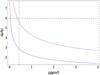 |
Fig. 1 Roche limit of Apophis as a function of its bulk density: the blue line corresponds to the rigid case, and the red curve to the fluid case. The dashed lines correspond to the minimum flyby distance. |
It is worth comparing the minimum distance during the close encounter (38 326 km) to the
Roche limit evaluated with respect to Earth, which is the minimum distance, measured from
the center of our planet, at which a secondary body is able to orbit without being destroyed
by the tidal forces of the first one. The Roche limit dR for Earth is
given by the following classical expression:  (1)where
RE
is the radius of the primary body (Earth), ρE its density, and ρA the density of
the orbiting body (Apophis). In Fig. 1, we plot the
value of the Roche limit for different values of Apophis’ density, which is still unknown,
but is generally taken between 2.6–2.8 g/cm3.
(1)where
RE
is the radius of the primary body (Earth), ρE its density, and ρA the density of
the orbiting body (Apophis). In Fig. 1, we plot the
value of the Roche limit for different values of Apophis’ density, which is still unknown,
but is generally taken between 2.6–2.8 g/cm3.
For this calculation, we use the mean radius of Earth, RE = 6371 km and an average density of ρE = 5.515g/cm3. For the density range above (ρA = [2.6–2.8]), Fig. 1 shows that the Roche limit is on the order of 1.6 RE, a distance that corresponds roughly to 26% of the minimum estimated distance of the encounter. For a density of ρA = 1 and ρA = 0.5, the Roche limit becomes 2.2RE and 2.8RE respectively, which correspond to 38% and 47% of this distance. Scheeres et al. (2005) mention the density of 0.44, for which the closest approach uncertainty ellipse lies within the Roche limit. According to our calculations, the nominal value of the closest distance (38 326 km) is still twice more than the nominal Roche limit.
As mentioned by Scheeres et al. (2005), if the asteroid’s bulk density is greater than 1, we can expect that the asteroid will most likely not disrupt catastrophically, but that for densities below this value, terrestrial torques should cause strong angular accelerations and particles on the surface should experience large fractional changes in local gravity.
3. Calculation of rotational changes during the close approach
The changes in the rotational motion of a celestial body in space are characterized by the variations of two components: the first one is the displacement of its polar axis with respect to an inertial frame, and the second is the variation in its angular velocity around its instantaneous axis of rotation. What we call the polar axis above is worth being clarified. In the case of Earth, the precision of the observations from modern techniques such as VLBI and GPS implies differentiating three polar axes: the axis of angular momentum, the axis of rotation, and the axis of figure. From an observational point of view, when at any time we want to accurately determine the rotational state of our planet, in principle only the determination of the polar axis of figure is necessary. To satisfy this requirement, a very accurate conventional model of precession-nutation motion for the figure axis of the Earth, called MHB2000, has been constructed by Mathews et al. (2002), taking non-rigid effects into account, such as geophysical ones. Nevertheless, for this purpose, it was previously necessary to compute a preliminary model of precession-nutation starting from a simplified rigid Earth model Bretagnon et al. (1998), Roosbeek & Dehant (1998), Souchay et al. (1999). Given the precision required, it was necessary for this computation to distinguish between the three polar axes mentioned above. In this paper we are dealing with a celestial object, Apophis, with poorly known physical and rotational parameters. Thus, there is no significant reason to distinguish between the figure axis, the angular momentum axis, and the rotational axis, which should be very close to each other, as for Earth. Moreover, Scheeres et al. (2005) show that the rotational index Ir which characterizes the departure of the axis of figure from the axis of rotation of Apophis, does not undergo drastic change, remaining close to Ir = 1 during the flyby, so that these axis are supposed to remain nearly coincident. Accepting that fact, we call the unique corresponding pole Pr.
3.1. Specificities of Apophis’ rotation
We use here a well established theoretical framework for computing the precession-nutation motion of a rigid body, set up by Kinoshita (1977) based on Hamiltonian formalism and canonical equations. This model has already been applied by Bouquillon & Souchay (1999) for the rotation of Mars and by Souchay et al. (2003) for the rotation of the asteroid (433) Eros, after the NEAR spacecraft touched its surface. The main difference with these previous studies holds in the relative motion of the body perturbing the rotation. In the case of Mars and Eros, the perturbing body is the Sun and the orbital motion of the studied object (Mars or Eros) is quasi-Keplerian (elliptic): therefore, the resulting expression of the solar perturbing potential is characterized by a Fourier series with arguments that are linear combinations of the mean anomaly of the object considered, and its mean longitude λ = M + ω + Ω (ω argument of perihelion, Ω longitude of the ascending node, and M the mean anomaly). In that case the motion of the polar axis is modeled as a combination of sinusoidal oscillations (the nutations) and of a secular motion (the precession).
By contrast, our study is significantly different. First we limit it to the few hours during the close approach, for which the trajectory of the perturbing body (Earth) with respect to the perturbed one (Apophis) is a quasi hyperbolic segment, in the framework of a two-body problem. As a consequence we consider the Apophis-Earth system as isolated, ignoring the solar gravitational influence, negligible in comparison, both from an orbital and a rotational point of view. As a consequence of these characteristics, we must treat the nature of perturbation of the rotation as the result of a gravitational impulse instead of a cyclic gravitational action.
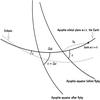 |
Fig. 2 Parameters used for the Apophis spin orientation in space. |
3.2. Parametrization and equations of motion
Here we represent the position of Apophis’ polar axis with respect to its orbital plane –
with respect to Earth – by a pair of parameters (ψ,ε), where
ψ is the
longitude of the ascending node γ of the orbital plane with respect to Apophis’
equatorial plane, and ε is Apophis’ obliquity, that is to say, the angle
between Apophis’ equatorial and orbital planes (see Fig. 2). This parametrization is the exact transposition of the classical one adopted
for the study of the rotation of Earth, where in this last case, the basic reference plane
is the orbital plane of our planet around the Sun, that is to say, the ecliptic. The
results for Apophis should not be significantly different when adopting the ecliptic as
reference plane, since Apophis’ inclination with respect to the ecliptic is only
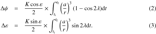
 (see Table 1). We call Δψ and Δε variations of the two
rotational parameters during the close approach, from an initial time ti to a final
one tf. To obtain their expressions at the
first order of the perturbing function we can rely on the classical work dealing with the
rotation of a rigid body (Kinoshita 1977). It is
based on a Hamiltonian formalism with canonical equations. The two variables in this
theoretical work concerned by our study are h = −ψ and I = −ε.
We can also use the formalism found in a previous direct application of this work for the
asteroid, i.e., 433 Eros (Souchay et al. 2003):
(see Table 1). We call Δψ and Δε variations of the two
rotational parameters during the close approach, from an initial time ti to a final
one tf. To obtain their expressions at the
first order of the perturbing function we can rely on the classical work dealing with the
rotation of a rigid body (Kinoshita 1977). It is
based on a Hamiltonian formalism with canonical equations. The two variables in this
theoretical work concerned by our study are h = −ψ and I = −ε.
We can also use the formalism found in a previous direct application of this work for the
asteroid, i.e., 433 Eros (Souchay et al. 2003):
 These
equations are established with the postulate that the rotation rate ω = 2π/T
is constant, which implies that K, which is proportional to period T, as shown below, has been
put outside the quadrature. As shown by Scheeres et al.
(2005), the value of rotation period should be affected by the flyby, but to a
rather small relative extent, less than 10% in view of the figure related to Monte Carlo simulations in this
paper. This explains why at first approximation we can set K as constant. Also some
components exist in the disturbing function with an argument that combines both the
longitude λ
and the angular angle ωt. They arise from the part of the disturbing
function due to the triaxiality (Kinoshita 1977)
and should be affected by the variation in ω during the flyby (Scheeres et al. 2005). But the presence of ωt in the argument gives
birth to high frequency terms that become, in comparison, very small after integration.
This explains why we do not take this part of the disturbing function into account.
These
equations are established with the postulate that the rotation rate ω = 2π/T
is constant, which implies that K, which is proportional to period T, as shown below, has been
put outside the quadrature. As shown by Scheeres et al.
(2005), the value of rotation period should be affected by the flyby, but to a
rather small relative extent, less than 10% in view of the figure related to Monte Carlo simulations in this
paper. This explains why at first approximation we can set K as constant. Also some
components exist in the disturbing function with an argument that combines both the
longitude λ
and the angular angle ωt. They arise from the part of the disturbing
function due to the triaxiality (Kinoshita 1977)
and should be affected by the variation in ω during the flyby (Scheeres et al. 2005). But the presence of ωt in the argument gives
birth to high frequency terms that become, in comparison, very small after integration.
This explains why we do not take this part of the disturbing function into account.
The integration is carried out within an interval of time for which the action of Earth is considered significant enough, during the close approach. Here, r stands for the distance between Apophis and Earth, and a is an arbitrary scaling constant value of the distance. When studying the Earth’s rotation Kinoshita (1977), Souchay et al. (1999), it is chosen as the semi-major axis of Earth (when studying the perturbation due to the Sun) or of the Moon (when studying the perturbation due to our satellite). The advantage of such a choice is to enable a development of (a/r) and (a/r)3 as a function of the eccentricity e and of the mean anomaly M of the relative motion of the perturbing body. In the present case of Apophis, such a development is not possible and not necessary anyway, because we concentrate our study on a few hours preceding and following the instant of closest approach. Thus we choose for a Apophis’ Earth MOID (Minimum Orbit Intersection Distance), that is to say: a = 0.00025619 au =38 326 km, according to the selected ephemerides, which will be detailed in Sect. 4.
The definition of the parameter λ needs to be clarified: λ is the true longitude of Earth measured from the ascending node γ. Although this ascending node is not known (since we do not know the orientation of the equator), λ can be determined from the ephemerides with a constant bias λ0 corresponding to the value of λ at the time t0 of the minimum of distance (Fig. 2). In our computations in the next section, we study the dependence of our results on the value of λ0.
3.3. The scaling factor K
The amplitude of Apophis’ rotational changes depends directly on the scaling factor
K in the
two Eqs. (2) and (3) above. K is given by 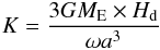 (4)where
G is the
gravitational constant, ME the mass of Earth, ω = 2π/T,
where T is
the period of rotation of the asteroid (T = 30.4 h). The only unknown parameter in the
above equation is Hd. It is given by
(4)where
G is the
gravitational constant, ME the mass of Earth, ω = 2π/T,
where T is
the period of rotation of the asteroid (T = 30.4 h). The only unknown parameter in the
above equation is Hd. It is given by 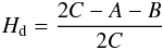 (5)where
A,
B, and
C represent
the moments of inertia of Apophis, with respect to the principal axes, with
A < B < C.
A reasonable value for Hd, when considering a recent study of
the distribution of this parameter over a set of 100 asteroids (Lhotka et al. 2013), is Hd = 0.2. This will be our nominal value
in the following.
(5)where
A,
B, and
C represent
the moments of inertia of Apophis, with respect to the principal axes, with
A < B < C.
A reasonable value for Hd, when considering a recent study of
the distribution of this parameter over a set of 100 asteroids (Lhotka et al. 2013), is Hd = 0.2. This will be our nominal value
in the following.
To understand the very large amplitude of the gravitational perturbing effect of the
Earth on the rotation of Apophis during the close approach, we can compare K with the corresponding
scaling factor  used in
computating the precession-nutation of Earth due to the Sun:
used in
computating the precession-nutation of Earth due to the Sun: 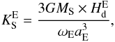 (6)where
 is the
dynamical ellipticity of our planet. Thus, when combining (4) and (6), the ratio
is the
dynamical ellipticity of our planet. Thus, when combining (4) and (6), the ratio
 is
given by
is
given by 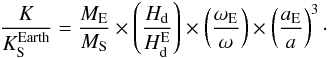 (7)Here
the comparatively very high value of K with respect to
is
essentially due, by far, to the last ratio in the equation: (aE/a)3 = 5.94721 × 10¹⁰.
When adopting Hd = 0.2, and by taking
(7)Here
the comparatively very high value of K with respect to
is
essentially due, by far, to the last ratio in the equation: (aE/a)3 = 5.94721 × 10¹⁰.
When adopting Hd = 0.2, and by taking
 (Souchay et al. 1999) we find K = 4.8167 × 10¹⁰′′/y which gives
 .
.
Indeed, in the case of Earth, the precession in longitude due to the Sun is on the order of 15′′/y. Therefore, because of the large ratio above, we can expect that despite the very short timescale of the flyby (a few hours), its effects on Apophis’ rotation could be dramatic, as confirmed in the next section.
4. Computations and results
The ephemerides used to compute the developments of the Apophis-Earth distance r, as well as the orientation angle λ used in Eqs. (2) and (3) were obtained by means of the tool Horizons, a service provided by the Jet Propulsion Laboratory (JPL ephemeris 2013). Our computations were carried out during an interval [−5 h, +5 h], with a 1 min time step. t = 0, the time of minimum of Apophis-Earth distance, corresponds to 2029 April 13 at 21:46 UT.
As explained in the previous sections, our results depend on three unknown parameters: the value of the dynamical ellipticity Hd of the asteroid, the original value of its obliquity ε before the encounter, and the value of Earth’s longitude λ0 measured from γ at t = 0. The amplitudes of the variations Δψ and Δε are directly proportional to Hd, so that they can be updated easily if we have a new estimate, different from our nominal value Hd = 0.2.
Our computations consist in simply numerically integrating the equations according to Eqs. (2) and (3). Because of the shortness of the interval, no specific integrator is necessary and we use a simple one. We obtain the values of λ − λ0 and r from the numerical ephemerides above.
In Figs. 3 and 4, we present the variations in Δψ and Δε during the interval [−5 h, +5 h] considered above. These variations are evaluated at the maximum cosε = 1 for Δψ and sinε = 1 for Δε, respectively. Moreover each curve in Figs. 3 and 4 corresponds to a given value of λ with a constant increment of π/8 (rad) in the interval λ0 = [0,π](rad).
We notice in Fig. 3 that, for all values of λ0, Δψ is positive and its amplitude is quite large, varying from 17°(× cosε) for λ0 = 0° to 31°(× cosε) for λ0 = 90° (π/2 rad).
In contrast, the post-encounter variations of the obliquity Δε (Fig. 4) are found in the interval ±7°(× sinε). Maxima correspond to the supplementary angles λ0 = 45° (π/4 rad) and λ0 = 135° (3π/4 rad). Also during the close approach, the amplitude of the variations can exceed these final values; for instance in the case λ0 = 22.5° (π/8 rad) and λ0 = 67.5° (3π/8 rad) half an hour after t = 0, where they reach ±10° × sinε. The values λ0 = 0 rad and λ0 = 90° (π/2 rad) present symmetric curves with no final variation in the obliquity, but a peak during the flyby reaching ±8°sinε. This corresponds to the cases for which the direction of Earth as seen from Apophis’ center at t = 0 crosses the nodal line γ, or is perpendicular to it.
Finally, the differential motion of Apophis’ spin axis in space during the close encounter can be represented at first approximation in the plane (Δψ × sinε,Δε). Therefore, for a given value of ε, the numerical results presented in Figs. 3 and 4 must be multiplied by sin2ε/2 and sinε, respectively. In Fig. 5 we represent the differential motion of the spin axis for two values of ε (ε = 20° in dashed lines, and ε = 45° in full lines) and four values of λ0 (λ0 = 0,45°,90°,135°). Therefore, for a given value of λ0, the curves are homothetical. Their characteristics (feature, amplitude, presence, and position of an inflection point) depend largely on the value of λ0. The largest amplitude, roughly 16°, is obtained for λ0 = 90° and ε = 45°.
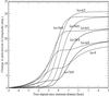 |
Fig. 3 Variations in Apophis’ precession in longitude during the close encounter with Earth, with Hd = 0.2 and various values of λ0. |
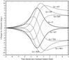 |
Fig. 4 Variations of Apophis’ obliquity during the close encounter with Earth, with Hd = 0.2 and various values of λ0. |
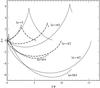 |
Fig. 5 Bi-dimensional motion of Apophis spin axis in space (Δε vs. Δψ × sinε) during the close encounter with the Earth, for ε = 45° (full) and ε = 20° (dashed). |
5. Discussion and conclusion
In this paper we have used a classical theory of the rotation of a celestial body under the gravitational perturbation exerted by an external body (Kinoshita 1977) to evaluate the rotational changes that Apophis might undergo during its close encounter with the Earth on April 13, 2029, at a distance of 38 326 km. We analyzed in particular the changes in orientation of Apophis’ polar axis starting from numerical integration during an interval of ten hours around the instant of closest distance. We show that our results depend directly on the values of three fundamental and still unknown parameters: the dynamical ellipticity Hd of the asteroid, its initial obliquity ε before the close encounter, and the longitude λ0 of the ascending node of the Apophis’ orbital plane with respect to Apophis’ equator. By taking a standard value Hd = 0.2, resulting from a statistical study of a set of 100 asteroids (Lhotka et al. 2013), we show that the changes in the orientation of Apophis’ polar axis in space will certainly reach several degrees during the flyby (see Fig. 5). This can be considered as very significant and could be easily detected from ground-based observations. In particular, our results should encourage undertaking specific radar experiments campaigns, following the same kinds of measurements as Ostro et al. (2004) in the case of (25143) Itokawa.
This constitutes a very challenging opportunity for detecting drastic rotational changes of a celestial body for the first time on a very short timescale. Moreover, we have shown in this paper that the variation profile in the pole’s orientation is highly dependent on λ0, whereas the amplitude, directly proportional to Hd is highly dependent on λ0 and ε. A big advantage of our calculations is that it is quite deterministic: we can adapt it automatically in the future to improved and more accurate knowledge of the value of λ0, ε, and/or Hd, which constrain the rotational changes presented here.
We recognize that our calculations here must be considered as approximate ones for several reasons: first, we only took the first order component of the disturbing potential of Earth into account, ignoring components due to the tri-axial shape of Apophis; second, we did not consider the effects of to the non-rigidity of the asteroid. Third, we did not consider, in the analytical calculation of the variations in the polar axis, that the spin rate should not show up constant during the flyby. Finally, we ignored the possible angular offset between the figure and the rotation axes. Indeed we postulate here that these kinds of contributions are significantly smaller than the effects considered in our the calculations, as is the case for planets in particular. Nevertheless, we recognize that more careful attention and more rigorous calculations that take the second order effects above into account should be made in a next paper.
We hope that by emphasizing the drastic possible changes of Apophis rotation during the 2029 encounter this paper will serve as a starting point for further studies related to this event, in particular concerning the rotation of the asteroid. Moreover, it could help for evaluating the post-encounter Yarkowsky effect in the best way, that will constrain the conditions of future flybys, as for the 2036 one.
Acknowledgments
The authors thank the anonymous referee for meticulous reviewing and very judicious comments, which helped improve the quality of the paper significantly.
References
- Bancelin, D., Colas, F., Thuillot, W., Hestroffer, D., & Assafin, M. 2012, A&A, 544, A15 [NASA ADS] [CrossRef] [EDP Sciences] [Google Scholar]
- Behrend, S. 2005, Asteroids and comets rotation curves, CdR, Observatoire de Genève, http://obswww.unige.ch/~behrend/page_cou.html, 2005 [Google Scholar]
- Benner, L. A. M. 2013, 99942 Apophis 2013 Goldstone Radar Observations Planning, http://echo.jpl.nasa.gov/asteroids/Apophis/Apophis_2013_planning.html, accessed on April 1st 2013 [Google Scholar]
- Binzel, R. P., Rivkin, A. S., Thomas, C. A., et al. 2009, Icarus, 200, 480 [NASA ADS] [CrossRef] [Google Scholar]
- Bouquillon, S., & Souchay, J. 1999, A&A, 345, 282 [NASA ADS] [Google Scholar]
- Bretagnon, P., Francou, G., Rocher, P., & Simon, J. L. 1998, A&A, 329, 329 [NASA ADS] [Google Scholar]
- Delbò, M., Cellino, A., & Tedesco, E. F. 2007, Icarus, 188, 266 [NASA ADS] [CrossRef] [Google Scholar]
- ESA 2013, Herschel intercepts asterpod Apophis, http://www.esa.int/Our_Activities/Space_Science/Herschel_intercepts_asteroid_Apophis, Jan. 2013 [Google Scholar]
- Farnocchia, D., Chesley, S. R., Chodas, P. W., et al. 2013, Icarus, 224, 192 [NASA ADS] [CrossRef] [Google Scholar]
- Giorgini, J. D., Benner, L. A. M., Ostro, S. J., Nolan, M. C., & Busch, M. W. 2008, Icarus, 193, 1 [NASA ADS] [CrossRef] [Google Scholar]
- JPL ephemeris 2013 http://ssd.jpl.nasa.gov/horizons.cgi, JPL ephemeris online generator [Google Scholar]
- Kinoshita, H. 1977, Celest. Mech., 15, 277 [Google Scholar]
- Lhotka, C., Souchay, J., & Shahsavari, A. 2013, A&A, 556, A8 [NASA ADS] [CrossRef] [EDP Sciences] [Google Scholar]
- Mathews, P. M., Herring, T. A., & Buffett, B. A. 2002, J. Geophys. Res., 107, 2068 [NASA ADS] [CrossRef] [Google Scholar]
- Nolan, M. 2013, Scheduled Arecibo Radar Asteroid Observations, http://www.naic.edu/~pradar/sched.shtml accessed on April 1st [Google Scholar]
- Ostro, S. J., Benner, L. A. M., Nolan, M. C., et al. 2004, Meteoritics, 39, 407 [Google Scholar]
- Roosbeek, F., & Dehant, V. 1998, Celest. Mech. Dyn. Astron., 70, 215 [NASA ADS] [CrossRef] [Google Scholar]
- Rubincam, D. P. 2007, Icarus, 192, 460 [NASA ADS] [CrossRef] [Google Scholar]
- Sansaturio, M. E., & Arratia, O. 2008, Earth Moon Planets, 102, 425 [NASA ADS] [CrossRef] [Google Scholar]
- Scheeres, D. J., Benner, L. A. M., Ostro, S. J., et al. 2005, Icarus, 178, 281 [NASA ADS] [CrossRef] [Google Scholar]
- Sokolov, L. L., Bashakov, A. A., Borisova, T. P., et al. 2012, Sol. Syst. Res., 46, 291 [NASA ADS] [CrossRef] [Google Scholar]
- Souchay, J., Loysel, B., Kinoshita, H., & Folgueira, M. 1999, A&AS, 135, 111 [NASA ADS] [CrossRef] [EDP Sciences] [Google Scholar]
- Souchay, J., Kinoshita, H., Nakai, H., & Roux, S. 2003, Icarus, 166, 285 [NASA ADS] [CrossRef] [Google Scholar]
All Tables
All Figures
|
Fig. 1 Roche limit of Apophis as a function of its bulk density: the blue line corresponds to the rigid case, and the red curve to the fluid case. The dashed lines correspond to the minimum flyby distance. |
| In the text | |
|
Fig. 2 Parameters used for the Apophis spin orientation in space. |
| In the text | |
|
Fig. 3 Variations in Apophis’ precession in longitude during the close encounter with Earth, with Hd = 0.2 and various values of λ0. |
| In the text | |
|
Fig. 4 Variations of Apophis’ obliquity during the close encounter with Earth, with Hd = 0.2 and various values of λ0. |
| In the text | |
|
Fig. 5 Bi-dimensional motion of Apophis spin axis in space (Δε vs. Δψ × sinε) during the close encounter with the Earth, for ε = 45° (full) and ε = 20° (dashed). |
| In the text | |
Current usage metrics show cumulative count of Article Views (full-text article views including HTML views, PDF and ePub downloads, according to the available data) and Abstracts Views on Vision4Press platform.
Data correspond to usage on the plateform after 2015. The current usage metrics is available 48-96 hours after online publication and is updated daily on week days.
Initial download of the metrics may take a while.