| Issue |
A&A
Volume 563, March 2014
|
|
|---|---|---|
| Article Number | A67 | |
| Number of page(s) | 13 | |
| Section | Numerical methods and codes | |
| DOI | https://doi.org/10.1051/0004-6361/201321958 | |
| Published online | 12 March 2014 | |
Performance improvements for nuclear reaction network integration
1
Departament de Física i Enginyeria Nuclear, EUETIBUniversitat Politècnica
de Catalunya
c/ Comte d’Urgell 187
08036
Barcelona
Spain
e-mail:
This email address is being protected from spambots. You need JavaScript enabled to view it.
2
Institut d’Estudis Espacials de Catalunya (IEEC),
Ed. Nexus-201, C/ Gran Capità
2-4, 08034
Barcelona,
Spain
3
Now at Department of Physics and Astronomy, University of North
Carolina, Chapel Hill
NC
27599-3255,
USA
Received:
24
May
2013
Accepted:
17
January
2014
Abstract
Aims. The aim of this work is to compare the performance of three reaction network integration methods used in stellar nucleosynthesis calculations. These are the Gear’s backward differentiation method, Wagoner’s method (a 2nd-order Runge-Kutta method), and the Bader-Deuflehard semi-implicit multi-step method.
Methods. To investigate the efficiency of each of the integration methods considered here, a test suite of temperature and density versus time profiles is used. This suite provides a range of situations ranging from constant temperature and density to the dramatically varying conditions present in white dwarf mergers, novae, and X-ray bursts. Some of these profiles are obtained separately from full hydrodynamic calculations. The integration efficiencies are investigated with respect to input parameters that constrain the desired accuracy and precision.
Results. Gear’s backward differentiation method is found to improve accuracy, performance, and stability in integrating nuclear reaction networks. For temperature-density profiles that vary strongly with time, it is found to outperform the Bader-Deuflehard method (although that method is very powerful for more smoothly varying profiles). Wagoner’s method, while relatively fast for many scenarios, exhibits hard-to-predict inaccuracies for some choices of integration parameters owing to its lack of error estimations.
Key words: methods: numerical / nuclear reactions, nucleosynthesis, abundances
© ESO, 2014
1. Introduction
Stellar models are an integral part of astrophysics that help us understand the structure and evolution of stars and their nucleosynthesis output. In order to properly resolve the wide range of conditions within these environments, models must be computed with high resolution in both space and time. Stellar models rely on a number of conservation equations (i.e., mass, energy, momentum) and energy transport mechanisms (i.e., radiation, convection, and conduction), which depend on the physical condition of the star. Further complicating these models, energy generation through nuclear reactions must be taken into account. Depending on the number of isotopes and nuclear interactions involved, these reactions can become very computationally expensive. Time evolution of hydrodynamical models is sometimes restricted, therefore, by the solution of a large system of ordinary differential equations that describe the network of nuclei in the star. If detailed nuclear reaction networks are desired, hydrodynamic models of the stellar system under investigation can be slowed to the point that they are no longer viable without high power supercomputers, unless post-processing techniques are employed.
The network of nuclei and reactions required in nucleosynthesis investigations can be divided into two broad nuclear reaction networks: (i) that which is responsible for energy generation and is therefore essential for any accurate hydrodynamical evolution of the system; examples of these networks were presented by Weaver et al. (1978); Mueller (1986); Timmes et al. (2000); and (ii) a reaction network that is only necessary for detailed computation of nucleosynthesis. This second network then uses, as input physics, the hydrodynamical properties of a plasma (i.e., temperature and density) obtained from a separate code using a limited set of reactions. De-coupling the networks in this way allows us to compute the expensive hydrodynamical model only once1, the output of which can be used to perform many post-processing calculations. The advantages of this approach are especially obvious for nucleosynthesis sensitivity studies (see, for example, Hix et al. 2003; Roberts 2006; Parikh et al. 2008). This method of de-coupling the nuclear reaction networks assumes that any nucleosynthesis occurring in the second step does not affect the behaviour of the hydrodynamical models in the first. In some cases, this decoupling of hydrodynamical models from nucleosynthesis networks is not valid. For example, the 1D implicit hydrodynamic code “SHIVA” (José et al. 1999) considered here integrates a network of over 1400 nuclear processes and several hundred isotopes into models of X-ray bursts, making nucleosynthesis a considerable bottleneck in the computational efforts. With these restrictions in mind, improving the reaction network integration performance is desirable in either of the cases described above, whether it is allowing larger step-sizes in full hydrodynamical models or increasing post-processing performance. Since full 1D hydrodynamic models are time-consuming to compute owing to their high spacial resolution, we concentrate our efforts on post-processing calculations using temperature-density profiles obtained separately. This simplification allows us to perform a detailed investigation of the sensitivity of the integration method to parameters controlling accuracy and precision. Furthermore, it allows us to investigate the performance of the integration method for computing models of a wide range of astrophysical environments2.
Nuclear reaction networks are particularly difficult to integrate numerically because the ordinary differential equations governing their evolution are “stiff”. A set of equations is considered stiff if the solution depends strongly on small variations in some of the terms. Consequently, very small step-sizes are required to ensure solution stability when explicit methods are used3. For complex nuclear networks, these step-sizes can become unacceptably small. Implicit methods are usually used to alleviate these problems (Press et al. 2007). These difficulties faced in the numerical integration of nuclear reaction networks were identified and successfully conquered in the late 1960’s using a range of semi-implicit and implicit methods (Truran et al. 1967; Arnett & Truran 1969; Wagoner 1969; Woosley et al. 1973). While these methods allowed nuclear reaction network evolution to be performed, the techniques involved are rather primitive, and possible improvements have been largely ignored for 40 years.
While most nucleosynthesis reaction network codes still employ the methods mentioned above, some groundbreaking work has been done on investigating improved techniques. Timmes (1999) investigated a large number of linear algebra packages and semi-implicit time integration methods for solving nuclear reaction networks. The findings of that investigation were important not only in improving network integration efficiency, but also in characterising the accuracy of abundance yields. This second advantage is a key point in constructing more robust and flexible integration algorithms. One integration method that Timmes (1999) did not investigate, however, was Gear’s backward differentiation method (Gear 1971), which is a fully implicit method that utilises past history of the system of ordinary differential equations to predict future solutions, thus increasing the integration time-step that can be accurately taken.
It is the purpose of this paper to investigate a number of methods for integrating nuclear reaction networks in stellar codes. We will concentrate on 3 methods, namely Wagoner’s two-step method (Wagoner 1969), Gear’s backward differentiation method (Gear 1971), and the Bader-Deuflehard method (Bader & Deuflhard 1983). Wagoner’s method will be considered primarily because it is widely used in nuclear astrophysical codes, hence serving as a convenient baseline for comparison. Gear’s method has been utilised previously in a number of studies: in big bang nucleosynthesis (Orlov et al. 2000); explosive nucleosynthesis (Luminet & Pichon 1989); 26Al production Ward & Fowler (1980); and r-process calculations (Nadyozhin et al. 1998; Panov & Janka 2009), but its performance for a range of nucleosynthesis applications has never been fully investigated. Finally, the Bader-Deuflehard method was suggested by Timmes (1999), which was found to dramatically improve integration times for the profile considered in that work. Indeed, this method has been successfully used in a number of studies (e.g., Noël et al. 2007; Starrfield et al. 2012; Pakmor et al. 2012).
Each of the integration methods will be introduced in Sect. 2, for which we will highlight the important detail of step-size adjustment and error checking. The test suite of profiles and reaction networks will be introduced in Sect. 3, and the results of these tests presented in Sect. 4. Detailed discussion of the results is given in Sect. 5, paying attention to numerical reasons for any behavioural differences between the methods. Conclusions and recommendations are made in Sect. 6.
2. Integration methods
A large number of methods can be used for implicitly or semi-implicitly solving stiff systems of ordinary differential equations (see, for example, Press et al. 2007). In this work, we will concentrate on three of these possibilities: (i) Wagoner’s two-step integration technique (basically, a second order Runge-Kutta method), which is commonly known in numerical astrophysics (Wagoner 1969). This method hinges on taking a large number of computationally inexpensive time-steps to solve the system of equations; (ii) the Bader-Deuflehard method, which is a semi-implicit method that is based on taking computationally expensive time-steps, but offset by only requiring few of them; and (iii) Gear’s backward differentiation method, which uses previous history of the system of equations to predict future behaviour, thus allowing larger steps to be taken while preserving the fairly inexpensive individual steps exhibited by Wagoner’s method. Note that this final method is only applicable in cases where past history can be stored in this way.
For each of the integration methods discussed, the most computationally expensive procedure for reaction network integration is solving the system of equations that describes the rate of change of each nucleus as a function of every other nucleus. To perform this task, Timmes (1999) recommended the linear algebra package, MA28 . Since that time, an updated version to the package, MA48 (Duff & Reid 1996), has become available, which we use in the current investigation. Computational efficiency differences between the two are expected to be minor, with the main advantages of the new package being ease-of-use.
2.1. Wagoner’s method
What is often referred to as “Wagoner’s method” in nuclear astrophysics is outlined by Wagoner (1969). The method is a semi-implicit, second-order Runge-Kutta method, and represents an extension of the single-order method first used in Truran et al. (1967) and Arnett & Truran (1969). Below, we present an outline of the method to clarify notation, allowing easier comparison with the other methods discussed below.
To construct the system of ordinary differential equations, we first define a vector,
yn, which represents
the molar fraction of all nuclei in the network at time tn, i.e., yn = [Y1,Y2,...,Yi,max] n.
Here, the molar fraction of an isotope is defined as Yi = Xi/Ai,
where Xi is the mass fraction
and Ai is the atomic mass
of species i.
These abundances are advanced to time tn + 1 with a time-step
of h by
solving the equation: ![Mathematical equation: \begin{equation} \label{eq:wag1} y_{n+1} = y_n + \frac{1}{2} h \left[ \frac{{\rm d}y}{{\rm d}t}(y_n,t_n) + \frac{{\rm d}y}{{\rm d}t}(\tilde{y}_{n+1},t_{n+1}) \right], \end{equation}](/articles/aa/full_html/2014/03/aa21958-13/aa21958-13-eq10.png) (1)where
(1)where
 are the intermediate abundances evaluated at the future time, t + 1. The time derivatives
of y are
found by considering all reactions that produce and destroy each nucleus. These can be
split into three contributions: (i) decay processes involving single species; (ii)
two-body reactions of the form A(a,b)B; and
(iii) three-body reactions such as the triple-alpha process. Putting these together:
are the intermediate abundances evaluated at the future time, t + 1. The time derivatives
of y are
found by considering all reactions that produce and destroy each nucleus. These can be
split into three contributions: (i) decay processes involving single species; (ii)
two-body reactions of the form A(a,b)B; and
(iii) three-body reactions such as the triple-alpha process. Putting these together:
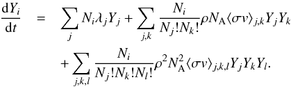 (2)Here
Ni is an absolute
number denoting the number of the species i that is produced in the reaction. Note that this
can be a negative number for destructive processes. The decay rate for species
i is given
by λi, ρ denotes the density of
the environment, NA is Avogadro’s number, and
⟨ σv ⟩ i,j is the
reaction rate per particle pair for two-body reactions involving species i and j. Three-body reaction
rates follow the same notation see (see Iliadis
2007, for a more detailed discussion).
(2)Here
Ni is an absolute
number denoting the number of the species i that is produced in the reaction. Note that this
can be a negative number for destructive processes. The decay rate for species
i is given
by λi, ρ denotes the density of
the environment, NA is Avogadro’s number, and
⟨ σv ⟩ i,j is the
reaction rate per particle pair for two-body reactions involving species i and j. Three-body reaction
rates follow the same notation see (see Iliadis
2007, for a more detailed discussion).
Equation (1) is solved using a two-step
procedure in which the second part of the equation depends on the first part through
:
 (3)To ameliorate numerical
instabilities arising from solving these equations explicitly, these equations are solved
implicitly. To achieve this, a Jacobian matrix must first be constructed. If
f(yn,tn) ≡ dyn/dt,
then the Jacobian matrix is J = ∂f/∂y.
Using this, Eq. (3) can be re-written using
an implicit scheme and represented in matrix form by
(3)To ameliorate numerical
instabilities arising from solving these equations explicitly, these equations are solved
implicitly. To achieve this, a Jacobian matrix must first be constructed. If
f(yn,tn) ≡ dyn/dt,
then the Jacobian matrix is J = ∂f/∂y.
Using this, Eq. (3) can be re-written using
an implicit scheme and represented in matrix form by ![Mathematical equation: \begin{equation} \label{eq:wag3} \left[\mathbf{I} - h\mathbf{J}\right]\tilde{y}_{n+1} = y_n, \end{equation}](/articles/aa/full_html/2014/03/aa21958-13/aa21958-13-eq25.png) (4)where I is the unity matrix. This
equation is subsequently solved to obtain the new abundances,
and Eq. (1) is solved by performing this
operation twice. Solving Eq. (4) represents
the most computationally expensive operation in each of the methods considered here. This
large M × M matrix (where M is the number of nuclei
in the network) exhibits a characteristic sparse pattern. While, in principle, every
nucleus in the network can interact with every other, processes involving light particles
are far more likely owing to their smaller Coulomb barrier. Large portions of the matrix,
therefore, are essentially negligible. Typical dimensions of this matrix are, for example,
~100 × 100 for novae, or ~600 × 600 for X-ray bursts. These Jacobian patterns are discussed in
considerable detail by Timmes (1999). The solution
of these sparse systems is left to the well optimised MA48 routines
from the HSL Mathematical Software Library (Duff &
Reid 1996) in the present work. Since the solution of these large systems of
equations is by far the most expensive operation in integrating nuclear reaction networks,
reducing the total number of times this operation must be performed is the ultimate goal
when attempting to increase algorithm efficiency. However, we must develop ways to ensure
that safe step-sizes are used to obtain accurate results.
(4)where I is the unity matrix. This
equation is subsequently solved to obtain the new abundances,
and Eq. (1) is solved by performing this
operation twice. Solving Eq. (4) represents
the most computationally expensive operation in each of the methods considered here. This
large M × M matrix (where M is the number of nuclei
in the network) exhibits a characteristic sparse pattern. While, in principle, every
nucleus in the network can interact with every other, processes involving light particles
are far more likely owing to their smaller Coulomb barrier. Large portions of the matrix,
therefore, are essentially negligible. Typical dimensions of this matrix are, for example,
~100 × 100 for novae, or ~600 × 600 for X-ray bursts. These Jacobian patterns are discussed in
considerable detail by Timmes (1999). The solution
of these sparse systems is left to the well optimised MA48 routines
from the HSL Mathematical Software Library (Duff &
Reid 1996) in the present work. Since the solution of these large systems of
equations is by far the most expensive operation in integrating nuclear reaction networks,
reducing the total number of times this operation must be performed is the ultimate goal
when attempting to increase algorithm efficiency. However, we must develop ways to ensure
that safe step-sizes are used to obtain accurate results.
Safe step-sizes in Wagoner’s method are usually computed in an ad-hoc way based on the
largest abundance changes in the previous step. For example, the new step-size,
h′, can be computed using ![Mathematical equation: \begin{equation} \label{eq:newstep} h' = K h \left[\frac{y_{n+1}}{y_{n+1}-y_{n}}\right]_{\text{min}}, \end{equation}](/articles/aa/full_html/2014/03/aa21958-13/aa21958-13-eq33.png) (5)where
K is varied
by hand to ensure convergence of the final abundances. It typically assumes values between
0.1 and 0.4 (for the test suites in Sect. 3, a value
of K = 0.25
is adopted). To avoid small abundances dominating the step-size calculations, a parameter,
yt,min, is introduced. Only nuclei with
abundances greater than this value are used to calculate step-sizes, with others being
allowed to vary freely. Furthermore, a parameter can be introduced to limit the maximum
step-size, represented in our implementation by the parameter
Sscale, which controls the minimum number of time-steps
allowed. This parameter ensures that any sudden changes in the profile are not passed
unnoticed.
(5)where
K is varied
by hand to ensure convergence of the final abundances. It typically assumes values between
0.1 and 0.4 (for the test suites in Sect. 3, a value
of K = 0.25
is adopted). To avoid small abundances dominating the step-size calculations, a parameter,
yt,min, is introduced. Only nuclei with
abundances greater than this value are used to calculate step-sizes, with others being
allowed to vary freely. Furthermore, a parameter can be introduced to limit the maximum
step-size, represented in our implementation by the parameter
Sscale, which controls the minimum number of time-steps
allowed. This parameter ensures that any sudden changes in the profile are not passed
unnoticed.
While Wagoner’s method is slightly more advanced than a simple Euler method (see Timmes 1999), it still provides no good means of determining step accuracy. In order to ensure accurate integration, a combination of experience and conservatism is required, in which abundance changes and the rate of step-size increases are severely restricted. The only available method of checking solution accuracy is by considering the conservation of mass in the system. Once the total mass deviates outside a given tolerance (imposed by checking that ∑ Xi = 1), integration is assumed to have failed, and a new calculation with more restrictive integration parameters must be attempted.
2.2. Bader-Deuflehard semi-implicit method
The Bader-Deuflehard method (Bader & Deuflhard
1983; Timmes 1999; Press et al. 2007) relies on the semi-implicit mid-point rule:
![Mathematical equation: \begin{equation} \label{eq:midpoint-rule} \left[1-h\frac{\partial f}{\partial y}\right] \cdot y_{n+1} = \left[1-h\frac{\partial f}{\partial y}\right] \cdot y_{n-1} + 2 h \left[ f(y_n) - \frac{\partial f}{\partial y}\cdot y_n \right] \end{equation}](/articles/aa/full_html/2014/03/aa21958-13/aa21958-13-eq38.png) (6)where
f(yn)
is the time derivative of the isotopic abundance vector, yn, at time
tn. Rather than solving
this equation once per time-step, the adopted strategy is to solve several steps at once.
Consequently, one large step of length H can be taken in m sub-steps, each of length
h. The
method relies on the basic assumption that the solution following a step H is a function of the
number of sub-steps, which can be probed by solving the equations for a range of trial
values for m.
Once this function has been found, the solution can be extrapolated to an infinite number
of sub-steps, thus yielding converged abundances. Bader
& Deuflhard (1983) developed the sequence of m values that provides best
convergence, so the number of sub-steps is varied in the range: m = 2,6,10,14,22,34,50.
After each attempt, the result is extrapolated to an infinite number of sub-steps until
accurate convergence (within some pre-defined tolerance) is obtained. For a specific value
of m, the
solution after a large step H is given by yn + 1 = yn + ∑ mΔm,
the sub-steps to be taken are:
(6)where
f(yn)
is the time derivative of the isotopic abundance vector, yn, at time
tn. Rather than solving
this equation once per time-step, the adopted strategy is to solve several steps at once.
Consequently, one large step of length H can be taken in m sub-steps, each of length
h. The
method relies on the basic assumption that the solution following a step H is a function of the
number of sub-steps, which can be probed by solving the equations for a range of trial
values for m.
Once this function has been found, the solution can be extrapolated to an infinite number
of sub-steps, thus yielding converged abundances. Bader
& Deuflhard (1983) developed the sequence of m values that provides best
convergence, so the number of sub-steps is varied in the range: m = 2,6,10,14,22,34,50.
After each attempt, the result is extrapolated to an infinite number of sub-steps until
accurate convergence (within some pre-defined tolerance) is obtained. For a specific value
of m, the
solution after a large step H is given by yn + 1 = yn + ∑ mΔm,
the sub-steps to be taken are: ![Mathematical equation: \begin{eqnarray} \label{eq:BaderStepping} && k=0 \quad \Delta_0 = \left[1-h\frac{\partial f}{\partial y}\right]^{-1} \!\!\!\!\cdot h f(y_0) \\ && k=1 \ldots m-1 \quad \Delta_k = \Delta_{k-1} + 2 \left[1-h\frac{\partial f}{\partial y}\right]^{-1} \!\!\!\!\cdot h (f(y_k) - \Delta_{k-1})\quad\quad\quad \\ && k=m \quad \Delta_m = \left[1-h\frac{\partial f}{\partial y}\right]^{-1} \!\!\!\!\cdot h (f(y_m) - \Delta_{m-1}). \end{eqnarray}](/articles/aa/full_html/2014/03/aa21958-13/aa21958-13-eq44.png) If
no convergence is reached with m = 50, the step is re-attempted with a smaller
step-size, H.
This takes into account cases in which local environment changes occur within the step
(i.e., there is a sharp temperature change in the stellar environment). In these cases,
the assumption that the extrapolated solution is a function of m is no longer valid, so
smaller steps must be attempted until convergence is obtained.
If
no convergence is reached with m = 50, the step is re-attempted with a smaller
step-size, H.
This takes into account cases in which local environment changes occur within the step
(i.e., there is a sharp temperature change in the stellar environment). In these cases,
the assumption that the extrapolated solution is a function of m is no longer valid, so
smaller steps must be attempted until convergence is obtained.
Obviously, this method requires that the system of equations is solved a large number of times, and even for the best case scenario, convergence is reached when m = 6. In the worst case, when m = 50, a total of 138 Lower Upper (LU) matrix decompositions must be performed to take a single step. This method, therefore, relies on large steps to offset their computational cost (see Timmes 1999).
Error estimation and step-size adjustment for the Bader-Deuflehard method must also be
considered. The error estimate, ϵk, at the current
sub-step order k, is estimated directly by the polynomial
extrapolation truncation error (see Chap. 3 of Press et
al. 2007). Consequently, if the desired accuracy is ϵ, the new step-size,
Hk, for this order can
be estimated by  (10)However, we must
consider the work required to reach convergence for different values of k. The number of function
evaluations (expected to dominate the computational cost of the method) required to
compute a step is Ak + 1. The work
required per unit time-step of order, k, is therefore
(10)However, we must
consider the work required to reach convergence for different values of k. The number of function
evaluations (expected to dominate the computational cost of the method) required to
compute a step is Ak + 1. The work
required per unit time-step of order, k, is therefore  (11)where the
current step-size H is used to normalise the calculation. The order
used to estimate the next step-size is chosen by identifying the value of k′ that
minimises Wk. The new time-step
is then computed using this value for Hk′ in Eq.
(10).
(11)where the
current step-size H is used to normalise the calculation. The order
used to estimate the next step-size is chosen by identifying the value of k′ that
minimises Wk. The new time-step
is then computed using this value for Hk′ in Eq.
(10).
When performing the above calculations, it is customary to scale the calculated errors
for each nucleus by their abundance to obtain relative errors,
 , to be used in Eq.
(10). However, we do not wish to weight
nuclei with very small abundances equally in these step-size calculations, so an
additional parameter, yscale, is introduced. For abundances
below this value, relative errors are normalised to yscale such
that:
, to be used in Eq.
(10). However, we do not wish to weight
nuclei with very small abundances equally in these step-size calculations, so an
additional parameter, yscale, is introduced. For abundances
below this value, relative errors are normalised to yscale such
that:  (12)
(12)
2.3. Gear’s backward differentiation method
The backward differentiation method developed by Gear (1971) hinges on using past behaviour of the system to predict the solution at future times. Following that prediction, Newton-Raphson iteration is used to correct the solution until a predefined precision is reached. The advantage of this method is that it allows an increase in possible step-size, while maintaining a limited number of matrix LU-decompositions. For a good discussion of the method, including the particular implementation of Gear’s method adopted in the present paper, the reader is referred to Byrne & Hindmarsh (1975). Here, we discuss the key characteristics of the method.
Gear’s method hinges on updating and storing a qth order vector of past behaviour known as the
Nordsieck vector (Nordsieck 1961), zn, defined at each time
tn as ![Mathematical equation: \begin{equation} \label{eq:nord} z_n=\left[y_n, h\dot{y}_n, h^2\ddot{y}_n, \ldots, \frac{h^q y_n^{(q)}}{q!}\right]\cdot \end{equation}](/articles/aa/full_html/2014/03/aa21958-13/aa21958-13-eq62.png) (13)Here, yn is a vector of
abundances at the current time, h is the current step-size (i.e., h = tn + 1 − tn),
and
(13)Here, yn is a vector of
abundances at the current time, h is the current step-size (i.e., h = tn + 1 − tn),
and  are
the time derivatives of yn. To evolve the
system from time tn to tn + 1, the calculation
can be divided into two steps: (i) the predictor step; and (ii) the corrector step.
are
the time derivatives of yn. To evolve the
system from time tn to tn + 1, the calculation
can be divided into two steps: (i) the predictor step; and (ii) the corrector step.
For the predictor step, the Nordsieck vector is used to predict the future state of the
system:  (14)where A(q) is a
(q + 1) × (q + 1) matrix defined
by
(14)where A(q) is a
(q + 1) × (q + 1) matrix defined
by  (15)Following
this, the corrector step is taken. By defining a correction vector, en, as that required to
adjust the predicted
(15)Following
this, the corrector step is taken. By defining a correction vector, en, as that required to
adjust the predicted  abundances to the final solution yn + 1, the corrected
Nordsieck vector can be corrected using:
abundances to the final solution yn + 1, the corrected
Nordsieck vector can be corrected using:  (16)ℓ is computed using
 (17)where
 In
practice, these values are computed through a straightforward iterative procedure (Byrne & Hindmarsh 1975).
In
practice, these values are computed through a straightforward iterative procedure (Byrne & Hindmarsh 1975).
The correction vector is calculated using Newton-Raphson iteration. The procedure is to find the iterative correction, Δm, necessary to adjust each corrector step m until convergence reaches some predefined value. Therefore, we must solve:
![Mathematical equation: \begin{eqnarray} \label{eq:newton} && \left[ \mathbf{I} - \frac{h}{l_1} \mathbf{J}\right]\Delta^{(m)}= -(y_{n+1}^{(m)} - y_{n+1}^{(0)}) - \frac{h}{l_1} (f(y_{n+1}^{(m)}) - \dot{y}_{n+1}^{(0)}) \\ && y_{n+1}^{(m+1)} = y_{n+1}^{(m)} + \Delta^{(m)} . \end{eqnarray}](/articles/aa/full_html/2014/03/aa21958-13/aa21958-13-eq77.png) Here,
Here,
 is the
first time derivative of
is the
first time derivative of  , and
must be re-calculated at each corrector iteration. J is the Jacobian matrix,
J = ∂y/∂t,
evaluated using the predicted values calculated in Eq. (14). In principle, this matrix should be updated for each corrector
iteration step, but provided that the prediction is suitably close to the true solution,
updating J only
once per time-step is necessary. Typically, after only a few Newton-Raphson iterations,
solution convergence is achieved and Eq. (16) is used to correct the Nordsieck vector.
, and
must be re-calculated at each corrector iteration. J is the Jacobian matrix,
J = ∂y/∂t,
evaluated using the predicted values calculated in Eq. (14). In principle, this matrix should be updated for each corrector
iteration step, but provided that the prediction is suitably close to the true solution,
updating J only
once per time-step is necessary. Typically, after only a few Newton-Raphson iterations,
solution convergence is achieved and Eq. (16) is used to correct the Nordsieck vector.
While the method discussed so far can be used to solve numerical problems, automatic
step-size control cannot be achieved without some estimation of the step error. Following
successful convergence, the error can be estimated using the Taylor series truncation
error: ![Mathematical equation: \begin{equation} \label{eq:error} E_{n+1}(q) = \frac{1}{l_1}\left[ 1+\prod_{i=2}^{q}\left( \frac{t_{n+1} - t_{n+1-i}}{t_{n-1}-t_{n+1-i}} \right) \right]^{-1} e_{n+1}. \end{equation}](/articles/aa/full_html/2014/03/aa21958-13/aa21958-13-eq82.png) (22)Equation (22) can now be used to estimate the step-size
to be used in the following step. If ϵ is defined as the error tolerance per step, then
the new step-size is calculated in an analogous way to Eq. (10) by
(22)Equation (22) can now be used to estimate the step-size
to be used in the following step. If ϵ is defined as the error tolerance per step, then
the new step-size is calculated in an analogous way to Eq. (10) by 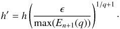 (23)This is usually
limited in practice by multiplying a conservative factor of 0.25 and by preventing large
changes in the step-size (Byrne & Hindmarsh
1975). In the same way as discussed for the Bader-Deuflehard method, relative
errors are calculated by scaling the errors by their corresponding abundances for those
larger than a pre-defined value yscale, as in Eq. (12).
(23)This is usually
limited in practice by multiplying a conservative factor of 0.25 and by preventing large
changes in the step-size (Byrne & Hindmarsh
1975). In the same way as discussed for the Bader-Deuflehard method, relative
errors are calculated by scaling the errors by their corresponding abundances for those
larger than a pre-defined value yscale, as in Eq. (12).
Beyond step-size estimation, the order of the method, q, can also be altered to
automatically select the most efficient method. Here, we follow the recommendation of
Byrne & Hindmarsh (1975) and allow only
order changes of q ± 1. Every so often (i.e., after at least
q steps at
the current order), trial error estimates are calculated for increasing and decreasing
order: ![Mathematical equation: \begin{eqnarray} E_{n+1}(q-1) &=& -\left[ \frac{\xi_1 \xi_2 \ldots \xi_{q-1}}{\ell_1(q-1)}\right] \frac{h^q y_{n+1}^{(q)}}{q!} \label{eq:errorqchangep}\\ E_{n+1}(q+1) &=& \frac{-\xi_{q+1} (e_{n+1} - Q_{n+1}e_{n})}{ (q+2)\ell_1(q+1)\left[1+\prod_2^q \frac{t_{n+1}-t_{n+1-i}}{t_n - t_{n+1-i}} \right]} \label{eq:errorqchangem} \end{eqnarray}](/articles/aa/full_html/2014/03/aa21958-13/aa21958-13-eq86.png) where
where
![Mathematical equation: \begin{eqnarray} \label{eq:Qeen} Q_{n+1} &=& \frac{C_{n+1}}{C_n}\left(\frac{h_{n+1}}{h_n}\right)^{q+1} \\ \label{eq:Ceen} C_{n+1} &=& \frac{\xi_1 \xi_2 \ldots \xi_{q}}{(q+1)!} \left[ 1+\prod_2^q \frac{t_{n+1}-t_{n+1-i}}{t_n - t_{n+1-i}} \right] \cdot \end{eqnarray}](/articles/aa/full_html/2014/03/aa21958-13/aa21958-13-eq87.png) By
using these expressions, trial step-sizes are found from Eq. (23). The largest step-size is then chosen and
the order altered accordingly if necessary. One final calculation is necessary before the
next time-step can be taken, and that is to scale the Nordsieck vector with the new
step-size and order. Order scaling is first applied. If the order is to increase or remain
constant, the Nordsieck vector requires no scaling. However, for reducing order, a factor
Δi must be subtracted from each column in
zn + 1,i,
where
By
using these expressions, trial step-sizes are found from Eq. (23). The largest step-size is then chosen and
the order altered accordingly if necessary. One final calculation is necessary before the
next time-step can be taken, and that is to scale the Nordsieck vector with the new
step-size and order. Order scaling is first applied. If the order is to increase or remain
constant, the Nordsieck vector requires no scaling. However, for reducing order, a factor
Δi must be subtracted from each column in
zn + 1,i,
where 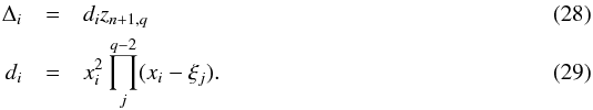 Regardless
of the order change, the Nordsieck vector must finally be scaled to the new step-size with
η = h′/h:
Regardless
of the order change, the Nordsieck vector must finally be scaled to the new step-size with
η = h′/h:
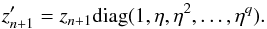 (30)Finally, once all of
these steps have been completed, the code returns to Eq. (14) and the next step is computed. This method automatically takes
care of starting steps, by using q = 1 until enough history has been built up to
utilise higher orders. It is fully automatic and although complicated, reduces the need
for expensive Newton-Raphson iteration by making beneficial use of past behaviour of the
system.
(30)Finally, once all of
these steps have been completed, the code returns to Eq. (14) and the next step is computed. This method automatically takes
care of starting steps, by using q = 1 until enough history has been built up to
utilise higher orders. It is fully automatic and although complicated, reduces the need
for expensive Newton-Raphson iteration by making beneficial use of past behaviour of the
system.
3. Input physics and test cases
To investigate the efficiency of each of the methods described in Sect. 2, a test suite of reaction networks and post-processing profiles is used. The purpose of these different cases is to investigate the performance of the integration schemes in a variety of nucleosynthesis post-processing situations. Different environments exhibiting different properties such as rapid changes of temperature or number of reactions involved are useful in highlighting the advantages and disadvantages of the methods described above.
3.1. Temperature and density profiles
Two flat profiles are used to explore the behaviour of the integration methods discussed here when no step-size limits related to profile behaviour are necessary. The first, referred to here as the “Flat” profile, is the same profile used by Timmes (1999), i.e., T = 3 × 10⁹ K and ρ = 2 × 10⁸ g/cm3 for 1 s. The second profile “Flat2” is a less extreme profile that is more applicable to novae, AGB stars, etc. In this case, the temperature and density are T = 3 × 10⁸ K and ρ = 2 × 10⁵ g/cm3 for 100 s.
The merger profile is extracted from Smoothed Particle Hydrodynamic (SPH) simulations (see, for example, Lorén-Aguilar et al. 2010) of white dwarf mergers and is shown in Fig. 1. For this particular model, the profile corresponds to a particular tracer particle in the merging of a 0.4 M⊙ helium white dwarf with a 0.8 M⊙ carbon-oxygen white dwarf. For this profile, the tracer particle was identified to exhibit significant nuclear reaction activity, and is therefore ideally suited for the present study. More details of this particular case can be found in Longland et al. (2011). The profile follows a characteristic shape. Initially, as material leaves the Roche lobe of the secondary white dwarf, the density and temperature drop. The material reaches and impacts the primary white dwarf’s surface (after about 14 s), undergoes rapid heating to T ≈ 1.5 × 10⁹ K in just a few seconds, and undergoes subsequent cooling on a timescale of around 10 s. The remainder of the profile is relatively cool, in which no nuclear processing occurs. This profile represents a post-processing situation in which the allowed time-step in nucleosynthesis integration is limited by the profile shape at early times, and not necessarily by theoretically allowed step-sizes computed by the integration method.
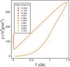 |
Fig. 1 Merger profile. Shown is the density plotted against the temperature with time represented by colour, with red for early times; yellow for late times. Time is labelled with respect to peak temperature, at which time, t = 0 s. Most of the nucleosynthesis is expected to occur, in this particular case, close to the start of the profile and within a 30 s window. |
To investigate the behaviour of the integration methods in nova nucleosynthesis, we use the temperature and density versus time profile of the innermost envelope shell, computed with the multi-zone 1D hydrodynamic code “SHIVA” (José et al. 1999). This model comprises of a 1.25 M⊙ ONe white dwarf accreting matter with solar metallicity at a rate of Ṁacc = 2 × 10⁻¹⁰ M⊙ yr-1. The profile, displayed in Fig. 2, was also used in the sensitivity study performed by Iliadis et al. (2002). As material is accreted from the companion star onto the white dwarf, density gradually increases on a long timescale (~1012 s) until conditions are reached in which explosive ignition of the material can occur. At that point, nuclear burning under degenerate conditions causes a rapid increase in temperature until degeneracy is lifted and the material subsequently expands and cools to settle at the end of the profile. This outburst stage occurs on a very short timescale (~1000 s) compared to the quiescent accretion phase of the profile. It is therefore essential to utilise an integration method that is capable of adaptive step-size control over a very large range of time-scales. Furthermore, the method must be capable of detecting loss of accuracy coming from sudden changes in nucleosynthesis, as we discuss in more detail later.
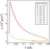 |
Fig. 2 Same as Fig. 1, but for the nova profile. This highlights the fact that the profile is relatively flat for most of the evolutionary history, with most of the nucleosynthesis occurring in a few thousand second window. |
Similarly, for X-ray burst nucleosynthesis, a temperature and density versus time profile is used from the innermost shell computed by the 1D SHIVA hydrodynamic code (José et al. 2010) and shown in Fig. 3. The burst is driven by accretion of solar metalicity material onto the surface of a 1.4 M⊙ neutron star at a rate of Ṁacc = 1.75 × 10⁻⁹ M⊙ yr-1. Similarly to the nova model discussed previously, for most of the profile, material undergoes compression and heating until conditions are reached at which nuclear burning begins after ~104 s. At this time, rapid heating and subsequent cooling of the material occurs in a 10 s window, followed by a quiescent settling period for a further ~104 s. This dramatic range of time-scales and conditions serves as a challenge to the network integration methods considered here.
Finally, in order to characterise the integration methods for a range of scenarios, an s-process profile (shown in Fig. 4) is used. The profile is extracted from the 1D hydrostatic core helium burning models of The et al. (2000), which follow the evolution of a 25 M⊙ star until helium is exhausted in the core. The profile is smoother than those of the nova and X-ray burst profiles and thus will probe a different numerical nucleosynthesis regime. The conditions over much of the profile are sufficient for helium burning to occur, but the s-process only becomes active at the end of the profile when the 22Ne + α neutron source is activated. This final profile provides a good test of situations for which there is continuous processing of material that changes in nature over time as opposed to the brief bursts of activity that are characterised by the nova, merger, and X-ray burst models.
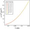 |
Fig. 4 Same as Fig. 1 but for the s-process profile. The times are scaled to the time at which helium is exhausted in the core. Once again, we see evolution approach the more complex nucleosynthesis region only for a relatively brief period at the end of the profile. |
3.2. The networks
Reaction rates in the present work are adopted from the starlib reaction rate library (summarised in Sallaska et al. 2013) for each network considered here. Each reaction rate is tabulated on a grid of temperatures between T = 10 MK and T = 10 GK. Cubic spline interpolation is used to compute the rate between temperature grid points. Since small nuclear networks do not present much of a challenge for modern computers, we only consider more detailed reaction networks here.
A large, 980 nucleus network (dubbed the “980” network in the following analysis) suitable for massive star nucleosynthesis is considered for both flat profiles discussed in Sect. 3.1. This network is based on the network presented by Woosley & Weaver (1995), but extended to barium. The network contains 9841 reactions linking nuclei from hydrogen to barium (Z = 56) with a 100% 4He initial composition. This represents a computationally more intensive network, requiring LU-decomposition of a 980 × 980 Jacobian matrix at every time-step.
The profile used to follow nucleosynthesis in merging white dwarfs is labelled the “Merger” network. This network is designed to allow for detailed nucleosynthesis studies from hydrogen to germanium (Z = 32), with a total of 328 isotopes and 3494 reactions. The initial mass fractions used in this particular network of 1H, 4He, and 3He are 0.5, 0.5, and 1 × 10⁻⁵, respectively. These initial abundances correspond to helium white dwarf buffer regions that are necessary to explain abundances in some hydrogen-poor stars (see Longland et al. 2011; Jeffery et al. 2011, and references therein).
The “Nova” network is based on that used by Iliadis et al. (2002) with initial abundances adopted from the JCH2 model in their Table 2. The network comprises of nuclei from hydrogen to calcium (145 isotopes) and 1274 reactions that allow for all common processes and their reverse reactions. Similarly, the “X-ray Burst” network is adopted from Parikh et al. (2008). It contains 813 nuclei up to xenon, linked by 8484 reactions. Initial abundances are defined for 89 of these nuclei similarly to those in Parikh et al. (2009). Both of these networks are modified only in that they include updated reaction rates from the starlib database.
Finally, the “s-Process” network is designed for studying the weak s-process in massive stars. A total of 341 nuclei are used from hydrogen to molybdenum, linked by 3394 reactions. The initial abundances are adopted from The et al. (2000), and correspond to the expected abundances prior to helium burning in a 25 M⊙ star.
4. Results
4.1. Integration times
To fully characterise the integration methods for the profiles and networks outlined in Sect. 3, the variables impacting integration accuracy constraints discussed in Sect. 2 are varied. Gear’s method and the Bader-Deuflehard method both use similar variables for controlling integration accuracy: yscale and ϵ. The first of these controls the normalisation of abundances when calculating integration errors through Eqs. (10) and (23). Relative errors are used to improve the accuracy of the integration routines for lower abundances. These are obtained by scaling truncation errors by the abundance for each isotope. The minimum abundance that this procedure is applied to is the integration variable yscale through Eq. (12). Scaling the abundances in this way results in a gradual decline in weight as abundances drop below this value, resulting in more stable integration performance.
No analog of these variables exists for Wagoner’s method in its present form. Historically, the accuracy of any one integration result is identified in an ad-hoc method that involves changing integration variables until the abundances of interest converge to stable values. Nevertheless, there are two variables, yt,min and Sscale, that are generally good indicators of the integration accuracy. yt,min controls the abundance below which no error checking is performed. Note that this is different from the yscale above, which still allows the method to use low abundance isotopes, but with less weight. In this case, yt,min represents a sharp cut-off. Sscale is a simple parameter that limits the maximum allowable step-size (i.e., larger values correspond to smaller time steps). This variable cannot be easily compared across usage situations, but within a single application, it can be used for characterising the method and guaranteeing that no sudden profile changes are missed by the integration method.
All tests were computed on a desktop PC with an 8-core Intel Core i7 2.67 GHz CPU. Only one core was utilised for all tests, ensuring that additional processes were kept to a minimum. However, all computation times presented here are normalised to the Wagoner’s method calculations with Sscale = 1000 and yt,min = 10-12 to remove most architecture specific computation dependence. Figures 6 to 11 show the total integration time required to compute nucleosynthesis for each of the test cases presented here as integration parameters are varied. In our integration method runs, we impose a 100 000 step limit on each test. This is to ensure that the tests are completed in a reasonable amount of time. When a method exceeds this limit, the approximate integration time can be inferred by extrapolating the curves.
4.2. Results convergence
Integration parameter reference table.
Comparing integration accuracy input parameters between methods is challenging. Using the same parameters for two different methods can, particularly for less constrained cases, lead to different accuracy in final results4. To account for this, we have performed additional tests as follows. Initially, a species in the network is chosen at the desired final abundance. For the following example, we consider the final abundance of 19F in the Nova test case, whose final abundance should be 3.5 × 10⁻⁸. The convergence behaviour of each method was then investigated according to the integration parameters outlined in Table 1. Results of the convergence tests are shown in Fig. 5 for the “Nova” profile and network.
It is clear from Fig. 5 that accurate results at the X ~ 10-8 level are not obtained for all integration parameters (many runs for the Wagoner method achieve results far outside the plotted region). For example, the “W04” run, corresponding to a Wagoner’s method run with Sscale = 10 and yt,min = 10-12 (see Table 1 for label interpretation) did not obtain an accurate result, with an error of about 30%. This procedure was repeated with varying precision requirements from X = 10-4 to X = 10-12 for all test cases considered here. For example, although test B14 exhibits converged results for this test case, it was not consistently accurate in others. By combining the results for all test cases, we obtained robust choices of representative integration parameters, which we consider to be “safe” for the purposes of this work. The representative integration parameters found are (i) Sscale = 1000, yt,min = 10-12 for Wagoner’s method; (ii) ϵ = 10-3, yscale = 10-10 for Gear’s method; and (iii) ϵ = 10-5, yscale = 10-15 for the Bader-Deuflehard method.
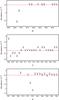 |
Fig. 5 Example of convergence tests for the “Nova” test case. See Table 1 for label interpretation. For example, point “G12” in the middle panel corresponds to a Gear’s method run with integration parameters of ϵ = 10-3 and yscale = 10-8. |
4.3. Bottleneck identification
It can also be illustrative to consider the fraction of time required by the most computationally intensive components of the calculations: (i) computation of the Jacobian matrix, which includes interpolating reaction rate tables; (ii) overhead required by the integration method; and (iii) linear algebra solution, which is dominated by matrix LU-decomposition as discussed in Sect. 2. The fraction of computation time used by each of these components was computed for representative integration variables for each method. The time-fractions required by each of these computation components are presented in Table 2. These were computed using the set of standard integration parameters found to provide comparable accuracy between methods. All absolute times have been normalised to the Wagoner’s method runs.
 |
Fig. 6 Run-times computed for case 1: “Flat”, and normalised to the Wagoner’s method calculation with Sscale = 1000 and yt,min = 10-12 (see text). Points indicated with a cross represent calculations that completed successfully with abundances that meet the accuracy criteria outlined in the text. Missing data points represent runs that did not successfully run, either arising from convergence problems within the code or from exceeding the maximum number of time-steps allowed. The labels “W”, “B”, and “G” represent run-times for Wagoner’s, the Bader-Deuflehard, and Gear’s methods, respectively. |
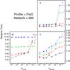 |
Fig. 7 Same as Fig. 6 but for case 2: the “Flat2” profile. Additionally, a closed circle symbol is used to represent runs that completed successfully but with results that do not meet the accuracy criteria outlined in the text. For example, the Wagoner’s method run for Sscale = 10 and Yt,min = 10-1 reports successful completion, but computes an abundance for 4He that exceeds the correct result by a factor of roughly 10. |
Relative computation times.
5. Discussion
5.1. Case 1: Flat
This computationally challenging flat profile represents hydrostatic helium burning in which helium is consumed to produce ashes largely consisting of 52Fe. As shown in Fig. 6, Wagoner’s method of integration requires a significant amount of fine tuning in order to successfully complete the evolution of the network for this profile. For large values of yt,min, the production of intermediate isotopes is not sufficiently accounted for in order to successfully complete the evolution. Convergence problems at later times are a consequence of this loss of accuracy, causing unrecoverable errors and premature exit from the code. Conversely, for small values of yt,min, convergence problems also arise. In this case, simplifications required in the semi-implicit method become invalid for nuclei with small abundances in the presence of rapidly changing nucleosynthesis flows. To achieve reasonable values of precision for this profile, integration parameters of Sscale = 1000 and yt,min = 10-8 are needed5. Using these parameters, full integration is completed successfully in 2500 s, with solution of equations being responsible for approximately 74% of that computation time. Recalculation of the Jacobian matrix in this case requires 20% of the computation time owing to the large number of steps required (over 70 000).
The Bader-Deuflehard method performs remarkably well for this flat profile (see also Timmes 1999). In very few time-steps, the method accurately completes integration over the profile. Furthermore, very small yscale and ϵ values can be safely used, resulting in rapid completion of the nucleosynthesis integration. This test highlights the power of the Bader-Deuflehard method when the profile is smoothly varying and the extrapolation method discussed in Sect. 2.2 can be used without additional step-size limitations. In comparison with Wagoner’s method above, we see in Table 2 that for our chosen set of integration parameters, the Bader-Deuflehard method successfully completes integration of the profile rapidly (just 85 s and 129 steps, just 3% of the time required by Wagoner’s method). This small number of integration steps explains why building the Jacobian matrix accounts for only 1% of the total computation time. The method overhead time, however, is relatively high from computing errors and step-size estimates. Note that even for extreme values for desired precision and accuracy, successful integration can be reached in a reasonable amount of time.
The Gear’s method for this profile performs remarkably well at large values of yscale and ϵ, completing evolution within 100 s. However, as these parameters increase, the time required for successful integration increases dramatically. At very small values of yscale and ϵ, evolution is not completed within the 100 000 step limit imposed in this work and computation is halted. For integration parameter values of yscale = 1 × 10⁻¹⁰ and ϵ = 1 × 10⁻³, the integration is completed in just over 326 seconds for this test case: roughly a factor of three slower than the Bader-Deuflehard method discussed above. Table 2 shows that, for these integration parameters, solution of the linear system of equations requires the most time (82% CPU time), with method overhead requiring about 6% of the computational time. The increased method overhead compared to Wagoner’s method is offset by the total time required for integration, just 326 s and 5000 steps.
5.2. Case 2: Flat2
In many nucleosynthesis situations, less extreme conditions are reached than those considered in the first flat profile. The computation times required by all three methods are shown in Fig. 7. Wagoner’s method performs considerably more stably for this profile than for the more extreme flat profile case. Here, the execution time depends weakly on yt,min, and rather depends quite strongly on Sscale, which effectively forces the code to take more steps than is necessary for this profile. Wagoner’s method seems to be sufficient for successful integration in this case. Using the standard choice of integration variables discussed above, computation time for this profile is just 64 s with solution of the linear system of equations requiring 66% of that time.
The Bader-Deuflehard method for this profile also performs well, with most choices of integration parameters resulting in completion times under 7 s. However, for the most extreme choices of yscale = 10-18 and ϵ = 10-6, a considerable increase is shown in Fig. 7 that corresponds to a comparatively large number of time-steps (~100 steps) needed by the accuracy constraints. This rapid increase highlights the poor performance of this method under scenarios requiring large numbers of time-steps. For more reasonable integration parameters, however, Table 2 shows that this method performs very well, requiring under one tenth of that needed by Wagoner’s method to complete integration over this profile.
Gear’s method also performs very well for this profile, with moderate dependence of execution time on both yscale and ϵ. Even for the most restrictive case using yscale = 10-16 and ϵ = 10-6, successful completion is still achieved in just 17 s. For the more reasonable parameters discussed before, the profile is successfully completed in 5 s. In this case, the method overhead (i.e., computing errors and estimating step-sizes) accounts for a large fraction of this time at 59%.
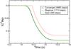 |
Fig. 12 Example of the importance in step error checking to reaction network integration. For Wagoner’s method (dashed line red), the algorithm can step past profile changes and therefore incorrectly compute nucleosynthesis activity while retaining good conservation of mass (the main tool available for estimating accuracy). Gear’s method (dot-dashed green line), on the other hand, can detect these changes by calculating the truncation error of each step, and return for smaller steps in the case where convergence fails. The solid, black line represents a Wagoner’s method calculation using conservative integration parameters found to produce converged nucleosynthesis results. |
5.3. Case 3: merger
For the merger profile and network test case, results are presented in Fig. 8. It is immediately obvious that Wagoner’s method does not provide reliable results for the smallest values of Sscale = 10 chosen in this study, even when integration over the profile is completed without error. A good example of this effect is shown in Fig. 12, where Wagoner’s method using small values of Sscale successfully steps past sudden profile changes, yielding inaccurate nucleosynthesis compared to our converged results obtained using a set of carefully chosen parameters. These are obtained by first picking restrictive integration parameters, and then varying those parameters to ensure that final abundances do not vary significantly. The smooth behaviour of the converged results in Fig. 12 also indicates that convergence is reached in this case. This failure to detect sudden changes in the profile stems from the lack of true error checking in this method. In this example, a large step is taken from 13.7 s to 14.5 s using an intermediate point at 14.1 s, where the temperature has not yet changed, thus leading to unchanged abundances. It is not until the following step, therefore, that high nuclear interaction activity is found. At that point, no good mechanism is implemented for automatically reversing the evolution by multiple time-steps to re-attempt integration over rapidly varying profiles. For our set of safe parameters discussed previously, however, Wagoner’s method does reach accurate abundance values in 115 s and about 27 000 steps. Two thirds of the computation time is used for solving the linear system of equations, with the other third used for rate calculation and method overhead.
The Bader-Deuflehard method exhibits interesting properties for this merger profile. It is immediately apparent that longer computation times are required to accurately integrate the network over this profile. This problem arises from the shape of the profile (Fig. 1). The dynamic, rapidly changing nature of the merger profile means that the infinite sub-step result of the Bader-Deuflehard method does not satisfactorily reach convergence for large time-steps. The shape of the profile changes so quickly that small steps must be taken to achieve convergence, thus erasing the benefit of the method. For our safe integration parameter choices, for example, 790 steps are required. While this represents half the number of steps required by Gear’s method for this profile, and only a small fraction of the number of steps required by Wagoner’s method, the expense of each step causes total integration time to be 335 s, almost 8 times that required by Gear’s method and over twice the time required by Wagoner’s method. Table 2 shows that most of this computation time is used to calculate rates (~40%) and solve the systems of equations (~60%).
Gear’s method successfully completes evolution with final abundances in agreement with the converged abundances for all cases except the most extreme yscale and ϵ values. Those cases failed because the step count exceeded the 100 000 step limit imposed in this study. The method’s behaviour follows a predictable pattern with more precise evolution requiring more time. Integration parameter values of yscale = 1 × 10⁻¹⁰ and ϵ = 1 ×10⁻³ yielded an integration time of 42 s in about 2800 steps, representing a speed-up factor of approximately 3 over Wagoner’s method for similar result accuracy. For this case, the method overhead is larger, but the reward in total computation time is clear.
5.4. Case 4: nova
Consider the Wagoner’s method run-times in Fig. 9. Some immediate observations can be made. Small values of Sscale (Sscale = 10, 100) cause nucleosynthesis completion apparently successfully, but as the small data points indicate, the abundances obtained from these runs disagree with converged values. Furthermore, it is difficult to predict which combinations of parameters will complete the evolution successfully. For example, the combination of Sscale = 1000 and yt,min = 10-8 reaches accurate abundances, but when yt,min = 10-10, incorrect abundances are obtained. Only three of the 7 runs with Sscale = 104 reached accurate abundances. The method accuracy can be tweaked using other integration parameters, but this example highlights some of the pitfalls of using network integration methods that do not include reliable error estimates. For our choice of safe integration parameters, however, reasonably accurate results for abundances X > 10-8 are obtained in just 3 s.
As was the case with the merger profile, the rapidly changing nova profile limits the step-size available to the Bader-Deuflehard method. These limited step-sizes result in very long computation times when using the Bader-Deuflehard method for nova profiles. None of the integration parameter sets considered here exceeded the 100 000 step limit imposed in our study. For our safe choice of parameters, successful profile integration was achieved in 34 s and 1200 steps. In this case, rate computation was a computationally expensive part of the calculation, requiring 36% of the time and indicating that many sub-steps were required to reach convergence.
Gear’s method follows a much more predictable pattern than Wagoner’s method for this profile. It is immediately obvious that most computations complete the evolution successfully with values that agree with the converged values. Furthermore, the error checking routines in Gear’s method ensure that the code rarely exits successfully with inaccurate results outside the range dictated by our input parameters. This is the immediate benefit of using reliable truncation error estimates to constrain the method. The computation time required for these profiles is similar to Wagoner’s method, with run-time for our chosen set of integration parameters taking just 2.8 s. Roughly half of this time is used for solving the systems of equations while rate calculation and method overhead account for 28% and 16%, respectively. The total number of LU-decompositions for this method is similar to that of Wagoner’s method resulting in an integration time improvement of only 20%, but it is clear that the benefit in this case come in the form of reliability.
5.5. Case 5: X-ray burst
The X-ray burst profile shape is qualitatively similar to that of the nova profile and thus, one would expect similar behaviour of the methods. However, the scope of nuclear activity during the profile dramatically changes the behaviour of Wagoner’s method with respect to the integration parameters shown in Fig. 10. For the largest values of yt,min, Wagoner’s method does not successfully complete integration of the network regardless of the Sscale value. In this case, the underlying reason is the same as that for the high temperature flat profile (see Fig. 6 and Sect. 5.1). That is, for large yt,min values, nucleosynthesis of less abundant species are not computed with enough accuracy. Consequently, once they do become abundant, the loss of accuracy at early times is propagated forward and mass conservation is broken in the system in an unrecoverable way. However, for more typical values of yt,min, the method is quite robust. Run-times follow a predictable pattern in which smaller values of yt,min require more time for integration. Interestingly, Sscale values of 100 and 1000 result in almost identical run-times. The reason for this is that for these cases, the actual time-steps taken for the two values are smaller than the maximum allowed by Sscale. This is expected behaviour for this integration method, although it is not easily predictable for a particular profile. For our choices of Sscale = 1000 and yt,min = 10-12, network integration is completed in 1300 s and 45 000 steps, highlighting the challenging nature of computing nucleosynthesis in X-ray bursts. Most of this time (69%) is required for solving the systems of equations, with rate calculations at each step taken 24% of the computation time.
The Bader-Deuflehard method behaves similarly for X-ray burst nucleosynthesis as for novae. For large ϵ values, convergence is achieved, but the time required is similar to that of Wagoner’s method. These run-times are explained similarly as for nova and merger profiles. The allowed time-step becomes limited by the profile rather than by the method itself. For small time-steps, the advantages of the method are outweighed by the large number of LU-decompositions necessary.
In direct contrast with the Bader-Deuflehard method, Gear’s method run times are remarkably fast for the X-ray burst model. Once again, the behaviour of run time as a function of the integration parameters follows a predictable pattern, but with small ϵ and yt,min combinations not fully completing integration within our maximum step limit. As Table 2 shows, integration over this profile takes about 240 s (~6100 steps) with reasonable parameters: over 5 times faster than Wagoner’s method and the Bader-Deuflehard method. With this choice of parameters, we find that the integration accuracy achieved is good down to the X = 10-12 level. The same pattern is found as before in which the method overhead is larger than it is for the other methods investigated in this work, but is offset by the robust and efficient performance overall.
5.6. Case 5: s-process
Finally, the s-process profile shown in Fig. 4 is considered, with integration times presented in Fig. 11. Wagoner’s method, once again, unsuccessfully complete nucleosynthesis integration over this profile for large values of yt,min. While in this case there are no sharp profile changes, there is a sudden nucleosynthesis activity change when the 22Ne + α reactions become active towards the end of the profile. Unless the evolution of nuclei is carefully accounted for at low abundance levels, they are not guaranteed to fulfil mass conservation requirements once they reach appreciable levels. However, for most higher values of yt,min, Wagoner’s method performs rather well for this s-process nucleosynthesis profile. For our selection of safe integration parameters discussed before, for example, the profile is integrated over in 36 s and 5500 steps. Rate calculation times become important for these small computation times, totalling 36% of the total computation time.
The Bader-Deuflehard method varies in performance for this test case. While, for large values of yscale and ϵ, integration times are on par with those from Wagoner’s method, for the smallest values it can perform rather poorly. In this case, it is the nature of the nucleosynthesis itself that limits the optimal step-sizes required to achieve convergence in the routine. For values of ϵ = 10-6, the Bader-Deuflehard method requires up to a factor of 10 times more computational time than Wagoner’s methods to complete nucleosynthesis integration. For our representative set of integration parameters, this method is about 2.5 times slower than Wagoner’s method.
Gear’s method in this case follows much the same behaviour as for other cases. Once again, the most extreme cases of small yscale and ϵ require many small time-steps that exceed the limits adopted in this work. For more reasonable values, however, computation times are comparable with Wagoner’s method, although a larger fraction of this time is required for solving the linear systems of equations. For our representative integration parameters, the Gear’s method requires 20 s in 1800 steps, highlighting the relative cost of each step in the method in comparison to Wagoner’s method, although still performing the integration twice as fast.
6. Conclusions
Integration of nuclear reaction networks has not received much modernisation since the first stellar modelling codes were developed over 4 decades ago. Now that computational power is becoming more available, it is possible to compute models in a relatively short period of time, thus opening avenues for detailed studies of the effects of varying model parameters. It is worth re-visiting the question of integration method efficiency to implement faster, more reliable nucleosynthesis solvers.
In this work, we tested the performance of two integration methods: the Bader-Deuflehard method and Gear’s backward differentiation method in comparison to the traditionally used Wagoner’s method. To fully investigate the behaviour of these integration methods, a suite of test profiles was used. This suite included 2 flat profiles, and profiles representing temperatures and densities in white dwarf mergers (helium burning), nova explosions (high temperature hydrogen burning), thermonuclear runaway, in X-ray bursts (the rp-process), and core helium burning in massive stars (He-burning and s-process nucleosynthesis).
In agreement with the findings of Timmes (1999), we found that although Wagoner’s method can sometimes be a fast way to integrate nuclear reaction networks, the lack of error estimates means that accuracy of the end results can be hard to predict. For more challenging cases such as nova or X-ray burst nucleosynthesis, great care must be taken to ensure accurate results. Even small variations in integration parameters can sometimes yield wildly varying results. The Bader-Deuflehard and Gear’s methods, on the other hand, rarely report inaccurate results at the precision desired through setting integration parameters. As reported in Timmes (1999), the Bader-Deuflehard method was found to be very powerful for flat profiles in which the step-sizes were only limited by the accuracy of the method. However, when dramatically varying temperature-density profiles were introduced, this was not necessarily the case, at least in a post-processing framework. Once small step-sizes are required to follow a sharp profile, the cost of each individual step in this method increases the computation time considerably. For simple profiles, or for use within a hydrodynamics code in which step-size can be safely increased to large values, this method is very robust and powerful.
Finally, Gear’s method was found to be very robust, only encountering difficulties for tight constraints on desired precision and accuracy. For all profiles in which the step-size was limited by a rapidly changing temperature and density, this method was found to out-perform both Wagoner’s and the Bader-Deuflehard methods. Furthermore, the speed of computation followed a clear trend with integration parameters, making it simple to use and easy to predict. The main disadvantage of this method is the difficulty in implementing it, since past behaviour must be stored in such a way to account for failed steps or changes of integration order. For more advanced applications, however, this method should be considered a powerful method for integrating nuclear reaction networks.
Summarising, we show that both the Bader-Deuflehard and Gear’s methods exhibit dramatic improvements in both speed and accuracy over Wagoner’s method used by many codes. Moreover, in applications for which the environment is expected to change rapidly, we found Gear’s method to be most robust and, thus, recommend its use in stellar codes.
Other techniques, such as parallelisation of hydrodynamic models can be of benefit in improving model computation time (Martin et al., in prep.).
However, any performance increases found in this work may also yield gains in computation time in full hydrodynamic models depending on the details of the code in question. This will be discussed in detail in a future paper.
For a recent and detailed discussion of improving the performance and stability of explicit methods, the reader is referred to Guidry (2012).
For the purpose of the tests performed here, we evaluate accuracy of results by comparing them with the most constrained calculations. Those have been carefully evaluated to ensure that convergence to stable results has been achieved for every isotope included in the network.
Note that the integration variables used to compare computation times for each of the other cases discussed here could not be used for this profile because they caused the computation to exceed our 100 000 step limit.
Acknowledgments
This work has been partially supported by the Spanish grants AYA2010-15685 and by the ESF EUROCORES Programme EuroGENESIS through the MICINN grant EUI2009-04167. We also thank the referee, Frank Timmes, for invaluable suggestions that helped to improve the manuscript.
References
- Arnett, W. D., & Truran, J. W. 1969, ApJ, 157, 339 [NASA ADS] [CrossRef] [Google Scholar]
- Bader, G., & Deuflehard, P. 1983, Numer. Math., 41, 373 [CrossRef] [Google Scholar]
- Byrne, G. D., & Hindmarsh, A. C. 1975, ACM Trans. Math. Softw., 1, 71 [CrossRef] [Google Scholar]
- Duff, I. S., & Reid, J. K. 1996, ACM Trans. Math. Softw., 22, 187 [CrossRef] [Google Scholar]
- Gear, C. W. 1971, Commun. ACM, 14, 176 [CrossRef] [Google Scholar]
- Guidry, M. 2012, J. Comput. Phys., 231, 5266 [Google Scholar]
- Hix, W., Smith, M., Starrfield, S., Mezzacappa, A., & Smith, D. 2003, Nucl. Phys. A, 718, 620 [NASA ADS] [CrossRef] [Google Scholar]
- Iliadis, C. 2007, Nuclear physics of stars (Wiley-VCH) [Google Scholar]
- Iliadis, C., Champagne, A., José, J., Starrfield, S., & Tupper, P. 2002, ApJS, 142, 105 [Google Scholar]
- Jeffery, C. S., Karakas, A. I., & Saio, H. 2011, MNRAS, 414, 3599 [NASA ADS] [CrossRef] [Google Scholar]
- José, J., Coc, A., & Hernanz, M. 1999, ApJ, 520, 347 [NASA ADS] [CrossRef] [Google Scholar]
- José, J., Moreno, F., Parikh, A., & Iliadis, C. 2010, ApJS, 189, 204 [NASA ADS] [CrossRef] [Google Scholar]
- Longland, R., Lorén-Aguilar, P., José, J., et al. 2011, ApJ, 737, L34 [NASA ADS] [CrossRef] [Google Scholar]
- Lorén-Aguilar, P., Isern, J., & García-Berro, E. 2010, MNRAS, 406, 2749 [NASA ADS] [CrossRef] [Google Scholar]
- Luminet, J.-P., & Pichon, B. 1989, A&A, 209, 85 [NASA ADS] [Google Scholar]
- Mueller, E. 1986, A&A, 162, 103 [NASA ADS] [Google Scholar]
- Nadyozhin, D. K., Panov, I. V., & Blinnikov, S. I. 1998, A&A, 335, 207 [NASA ADS] [Google Scholar]
- Noël, C., Busegnies, Y., Papalexandris, M. V., Deledicque, V., & El Messoudi, A. 2007, A&A, 470, 653 [NASA ADS] [CrossRef] [EDP Sciences] [Google Scholar]
- Nordsieck, A. 1961, On numerical integration of ordinary differential equations (University of Illinois, Coordinated Science Laboratory) [Google Scholar]
- Orlov, A. V., Ivanchik, A. V., & Varshalovich, D. A. 2000, Astron. Astrophys. Trans., 19, 375 [NASA ADS] [CrossRef] [Google Scholar]
- Pakmor, R., Edelmann, P., Röpke, F. K., & Hillebrandt, W. 2012, MNRAS, 424, 2222 [NASA ADS] [CrossRef] [Google Scholar]
- Panov, I. V., & Janka, H.-T. 2009, A&A, 494, 829 [NASA ADS] [CrossRef] [EDP Sciences] [Google Scholar]
- Parikh, A., José, J., Moreno, F., & Iliadis, C. 2008, ApJS, 178, 110 [Google Scholar]
- Parikh, A., José, J., Iliadis, C., Moreno, F., & Rauscher, T. 2009, Phys. Rev. C, 79, 045802 [NASA ADS] [CrossRef] [Google Scholar]
- Press, W., Teukolsky, S., Vetterling, W., & Flannery, B. 2007, Numerical recipes: the art of scientific computing (Cambridge University Press) [Google Scholar]
- Roberts, L. F. 2006, in Proc. International Symp. Nuclear Astrophysics – Nuclei in the Cosmos (CERN), 202 [Google Scholar]
- Sallaska, A. L., Iliadis, C., Champagne, A. E., et al. 2013, ApJS, 207, 18 [NASA ADS] [CrossRef] [Google Scholar]
- Starrfield, S., Iliadis, C., Timmes, F. X., et al. 2012, Bulletin of the Astronomical Society of India, 40, 419 [Google Scholar]
- The, L., El Eid, M. F., & Meyer, B. S. 2000, ApJ, 533, 998 [NASA ADS] [CrossRef] [Google Scholar]
- Timmes, F. X. 1999, ApJS, 124, 241 [NASA ADS] [CrossRef] [Google Scholar]
- Timmes, F. X., Hoffman, R. D., & Woosley, S. E. 2000, ApJS, 129, 377 [NASA ADS] [CrossRef] [Google Scholar]
- Truran, J. W., Arnett, W. D., & Cameron, A. G. W. 1967, Can. J. Phys., 45, 2315 [NASA ADS] [CrossRef] [Google Scholar]
- Wagoner, R. V. 1969, ApJS, 18, 247 [NASA ADS] [CrossRef] [Google Scholar]
- Ward, R. A., & Fowler, W. A. 1980, ApJ, 238, 266 [Google Scholar]
- Weaver, T. A., Zimmerman, G. B., & Woosley, S. E. 1978, ApJ, 225, 1021 [NASA ADS] [CrossRef] [Google Scholar]
- Woosley, S. E., & Weaver, T. A. 1995, ApJS, 101, 181 [NASA ADS] [CrossRef] [Google Scholar]
- Woosley, S. E., Arnett, W. D., & Clayton, D. D. 1973, ApJS, 26, 231 [NASA ADS] [CrossRef] [Google Scholar]
All Tables
All Figures
|
Fig. 1 Merger profile. Shown is the density plotted against the temperature with time represented by colour, with red for early times; yellow for late times. Time is labelled with respect to peak temperature, at which time, t = 0 s. Most of the nucleosynthesis is expected to occur, in this particular case, close to the start of the profile and within a 30 s window. |
| In the text | |
|
Fig. 2 Same as Fig. 1, but for the nova profile. This highlights the fact that the profile is relatively flat for most of the evolutionary history, with most of the nucleosynthesis occurring in a few thousand second window. |
| In the text | |
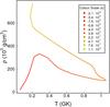 |
Fig. 3 Same as Fig. 1 but for the X-ray burst profile. |
| In the text | |
|
Fig. 4 Same as Fig. 1 but for the s-process profile. The times are scaled to the time at which helium is exhausted in the core. Once again, we see evolution approach the more complex nucleosynthesis region only for a relatively brief period at the end of the profile. |
| In the text | |
|
Fig. 5 Example of convergence tests for the “Nova” test case. See Table 1 for label interpretation. For example, point “G12” in the middle panel corresponds to a Gear’s method run with integration parameters of ϵ = 10-3 and yscale = 10-8. |
| In the text | |
|
Fig. 6 Run-times computed for case 1: “Flat”, and normalised to the Wagoner’s method calculation with Sscale = 1000 and yt,min = 10-12 (see text). Points indicated with a cross represent calculations that completed successfully with abundances that meet the accuracy criteria outlined in the text. Missing data points represent runs that did not successfully run, either arising from convergence problems within the code or from exceeding the maximum number of time-steps allowed. The labels “W”, “B”, and “G” represent run-times for Wagoner’s, the Bader-Deuflehard, and Gear’s methods, respectively. |
| In the text | |
|
Fig. 7 Same as Fig. 6 but for case 2: the “Flat2” profile. Additionally, a closed circle symbol is used to represent runs that completed successfully but with results that do not meet the accuracy criteria outlined in the text. For example, the Wagoner’s method run for Sscale = 10 and Yt,min = 10-1 reports successful completion, but computes an abundance for 4He that exceeds the correct result by a factor of roughly 10. |
| In the text | |
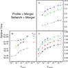 |
Fig. 8 Same as Fig. 6 but for case 3: the “Merger” profile. |
| In the text | |
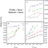 |
Fig. 9 Same as Fig. 6 but for case 4: the “Nova” profile. |
| In the text | |
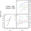 |
Fig. 10 Same as Fig. 6 but for case 5: the “X-ray burst” profile. |
| In the text | |
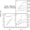 |
Fig. 11 Same as Fig. 6 but for case 6: the “S-Process” profile. |
| In the text | |
|
Fig. 12 Example of the importance in step error checking to reaction network integration. For Wagoner’s method (dashed line red), the algorithm can step past profile changes and therefore incorrectly compute nucleosynthesis activity while retaining good conservation of mass (the main tool available for estimating accuracy). Gear’s method (dot-dashed green line), on the other hand, can detect these changes by calculating the truncation error of each step, and return for smaller steps in the case where convergence fails. The solid, black line represents a Wagoner’s method calculation using conservative integration parameters found to produce converged nucleosynthesis results. |
| In the text | |
Current usage metrics show cumulative count of Article Views (full-text article views including HTML views, PDF and ePub downloads, according to the available data) and Abstracts Views on Vision4Press platform.
Data correspond to usage on the plateform after 2015. The current usage metrics is available 48-96 hours after online publication and is updated daily on week days.
Initial download of the metrics may take a while.