| Issue |
A&A
Volume 562, February 2014
|
|
|---|---|---|
| Article Number | L5 | |
| Number of page(s) | 4 | |
| Section | Letters | |
| DOI | https://doi.org/10.1051/0004-6361/201323009 | |
| Published online | 07 February 2014 | |
Simultaneous optical and near-infrared linear spectropolarimetry of the earthshine⋆
1
Instituto de Astrofísica de Canarias,
38205
La Laguna,
Spain
e-mail: This email address is being protected from spambots. You need JavaScript enabled to view it.
; This email address is being protected from spambots. You need JavaScript enabled to view it.
2
Departamento de Astrofísica, Universidad de La
Laguna, Av. Astrofísico Francisco
Sánchez, s/n, 38206
La Laguna,
Spain
3
Centro de Astrobiología (CSIC-INTA) , Carretera de Ajalvir km 4,
28850 Torrejón de Ardoz, Madrid, Spain
e-mail: This email address is being protected from spambots. You need JavaScript enabled to view it.
Received: 7 November 2013
Accepted: 23 January 2014
Abstract
Aims. We aim to extend our current observational understanding of the integrated planet Earth spectropolarimetry from the optical to the near-infrared wavelengths. Major biomarkers like O2 and water vapor are strong flux absorbents in the Earth’s atmosphere, and some linear polarization of the reflected stellar light is expected to occur at these wavelengths.
Methods. Simultaneous optical (0.4−0.9 μm) and near-infrared (0.9−2.3 μm) linear spectropolarimetric data of the earthshine were acquired by observing the nightside of the waxing Moon. The data have sufficient spectral resolution (2.51 nm in the optical, and 1.83 and 2.91 nm in the near-infrared) to resolve major molecular species present in the Earth’s atmosphere.
Results. We find the highest values of linear polarization (≥10%) at the bluest wavelengths, which agrees with other studies. Linear polarization intensity steadily decreases toward red wavelengths reaching a nearly flat value beyond ~0.8 μm. In the near-infrared, we measured a polarization degree of ~4.5 % for the continuum. We report the detection of molecular features due to O2 at 0.760,1.25 μm, and H2O at 0.653–0.725 μm, 0.780–0.825 μm, 0.93, and 1.12 μm in the spectropolarimetric data, and most of them show high linear polarimetry degrees above the continuum. In particular, the broad H2O 1.12 μm band displays a polarimetric intensity as high as that of the blue optical. These features may become a powerful tool for characterizing Earth-like planets in polarized light.
Key words: polarization / Moon / Earth / scattering
Reduced spectra (FITS Files) are only available at the CDS via anonymous ftp to cdsarc.u-strasbg.fr (130.79.128.5) or via http://cdsarc.u-strasbg.fr/viz-bin/qcat?J/A+A/562/L5
© ESO, 2014
1. Introduction
The increasing progress in instrumentation and observational techniques has allowed the detection of over 1000 planets with masses ranging from a few times the Jupiter mass to the super-Earth regime (≲10 M⊕). The most recent observational studies (e.g., Cassan et al. 2012) suggest that as many as 62% of the Milky Way stars can harbor Earth-like planets. It seems probable that a significant number of Earth-sized planets located within their parent stars’ habitable zones will be found in the near future.
Transit spectroscopy is currently the most extended technique for characterizing the planetary atmospheres of the new discoveries, and it has proved successful for gaseous giant planets (e.g., Swain et al. 2008). The atmospheres of Earth-sized planets are too difficult to study with actual instrumentation. While biomarkers are readily identifiable in the Earth’s transmission spectrum (Pallé et al. 2009), even in the most favorable case of an Earth-like planet orbiting small stars or brown dwarfs, several transits would be necessary for a reliable detection, even when using large-aperture (and space-based) telescopes (Kaltenegger & Traub 2009; Pallé et al. 2011). The probability of finding a transiting exo-Earth in the habitable zone of a G2V-type star is ~0.5% (Howard et al. 2012). The direct detection of the light reflected or emitted by the exo-Earth would be necessary for its proper characterization. This is indeed a very challenging task.
Polarization may contribute to the analysis of the atmospheres of these new worlds by taking advantage of the stellar light not generally being polarized, whereas the light reflected from the planet is. Various groups (Stam 2008; Karalidi et al. 2011) have done theoretically studies of the optical linear polarimetric signal of an Earth-like planet as a function of orbital phase and wavelength. Their predictions must be tested against observations of the only “Earth-like planet” known so far: the Earth. This can be done by observing the earthshine, which is the sunlight scattered by the dayside Earth and reflected by the nightside of the Moon. The optical and near-infrared earthshine spectra reveal atmospheric and surface biosignatures and are sensitive to features like water clouds, oceans, deserts, and volcanic activity (e.g., Woolf et al. 2002; Turnbull et al. 2006; Montañés-Rodríguez et al. 2006; Pallé et al. 2009; García Muñoz et al. 2012); many are present in the earthshine optical spectropolarimetric data (Sterzik et al. 2012; Takahashi et al. 2013).
Here, we provide the first linear spectropolarimetric measurements of the earthshine from the visible to the near-infrared (NIR) wavelengths (0.4−2.3 μm). We used observations of the Moon’s dark side to characterize the integrated polarimetric properties of the Earth. These observations extend our current understanding of the optical linear polarimetric data of the earthshine (Bazzon et al. 2013, and references therein) toward red wavelengths.
2. Observations and data analysis
Earthshine optical and NIR linear polarimetric spectra were taken using the Andalucía faint object spectrograph and camera (ALFOSC) of the 2.56-m Nordic Optical Telescope (NOT) and the long-slit intermediate-resolution infrared spectrograph (LIRIS; Manchado et al. 2004) of the 4.2-m William Herschel Telescope (WHT). The observing date was 2013 May 18; the journal of the observations is provided in Table 1.
ALFOSC polarimetric mode uses a calcite plate that provides simultaneous measurements of the ordinary and the extraordinary components of two orthogonally polarized beams separated by 15′′ and a half-wave plate that we rotated four times in steps of 22.5°. For spectroscopy we employed grism #4 and a slit 1 5 in width and ~15′′ long, which in combination with a pixel pitch of 019 (2048 × 2048 E2V detector), yield a wavelength coverage of ~0.4−0.9 μm and a spectral resolution of 2.51 nm (R ~ 250 at 0.65 μm).
LIRIS polarimetric mode uses a wedged double Wollaston device (Oliva 1997), consisting of the combination of two Wollaston prisms that deliver four simultaneous images of the polarized flux at vector angles 0° and 90°, 45° and 135°. An aperture mask 4′ × 1′ in size is in the light path to prevent overlapping effects between the different polarization vector images. Two retarder plates provide polarimetric images with exchanged orthogonal vector angles, useful for minimizing flat-fielding effects and providing better signal-to-noise (S/N) data (Zapatero Osorio et al. 2011; Miles-Páez et al. 2013). For spectroscopy we employed the grisms ZJ and HK and a slit 075 in width and 50′′ long, which in combination with a pixel size of 025 (1024 × 1024 HgCdTe HAWAII array), yield wavelength coverages of ~0.9−1.51 μm (ZJ) and ~1.4−2.4 μm (HK), and spectral resolutions of 1.83 nm (R ~ 540 at 1 μm) and 2.91 nm (R ~ 540,750 at 1.6 and 2.2 μm).
Spectropolarimetric observations were carried out under photometric sky conditions and raw seeing of 09. The angle formed by the Sun, the Moon, and the Earth was 81°, and the waxing Moon’s illuminated area was 59%. At the beginning of the astronomical night, the NOT and WHT were pointed to the center of the lunar disk, and an offset was applied to move both telescopes to the dark side (east) of the Moon. To track the Moon with the NOT during the observations, we manually introduced proper right ascension and declination rates1 every five minutes. The location of the ALFOSC and LIRIS slits on the Moon is illustrated in Fig. 1. Half of the LIRIS slit was positioned at the Moon terminator and the “dark” side, while the other half registered the sky contribution simultaneously. Because of the small size of the ALFOSC slit, alternate Moon and sky observations were conducted at a separation of 600′′.
One polarimetric cycle consisted of four consecutive frames with half-wave plate positions of 0°, 22°̣5, 45°, and 67°̣5 (ALFOSC), and two consecutive frames obtained with two different retarder plates (LIRIS). Typical exposure times per frame were 90 s and 400 s for the optical and NIR, and one full polarimetric cycle was thus completed in about 7 min (ALFOSC) and 14 min (LIRIS) including 0.5−1-min overheads. We collected a total of 15 cycles of earthshine polarimetric data, 7 cycles of “sky” observations with ALFOSC, and 6 (ZJ) and 4 (HK) cycles with LIRIS. Before sky subtraction, all LIRIS frames were rectified using the telluric emission lines and observations of Ar and Xe arcs so that the spatial axis lies perpendicular to the spectral axis. The earthshine ALFOSC data were sky subtracted using sky frames obtained very close in time and typically within ±0.1 airmass. Wavelength calibration was performed using observations of He+Ne (ALFOSC) and Ar+Xe (LIRIS) lamps, with a typical uncertainty of ±0.15−0.20 Å.
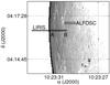 |
Fig. 1 Relative positions of the ALFOSC and LIRIS slits on the Moon surface during the observations of the lunar nightside on 2013 May 18. Equatorial coordinates α and δ correspond to 21h20m universal time. For displaying purposes, the slit widths are multiplied by a factor of four, and the slit lengths are plotted on true scale. |
Observing log (2013 May 18).
The normalized Stokes parameters q and u were computed using the flux ratio method and the equations given in Zapatero Osorio et al. (2005) for the optical and in Zapatero Osorio et al. (2011) for the NIR. We obtained as many q and u spectra as there were polarimetric cycles observed at optical wavelengths. To improve the S/N of the data, we present here final spectra computed by combining all polarimetric cycles and by collapsing all pixels along the spatial direction. A total of 65 ALFOSC pixels (or 1235) per wavelength were fused together into one-dimension spectra, while LIRIS data were folded up into two regions (indicated in Fig. 1): one (A, 39 pix or 975) close to the Moon terminator and another (B, 38 pix or 95) spatially near the location of the ALFOSC slit; each section corresponds to about one fourth of the total LIRIS slit length. In the collapsing processes, we obtained the average of all pixels and rejected the maximum and minimum values per wavelength. Optical data have better S/N than NIR spectra by factors of ~15 (optical versus ZJ) and ~25 (optical versus HK). The linear polarization degree was derived as the quadratic sum of the normalized Stokes parameters. The debiased polarization degree, p∗, was computed by considering the polarization uncertainty (see below) and according to the equation given in Wardle & Kronberg (1974).
Together with the earthshine data, observations of polarized and non-polarized standard stars (HD 154892, HD 161056, and Elia 2-25) from the catalogs of Schmidt et al. (1992) and Whittet et al. (1992) were acquired with the same instrumental configuration and on the same observing night as the earthshine, and were used to control the instrumental linear polarization and to check the efficiency of the ALFOSC and LIRIS optics. The same unpolarized standard was targeted at the two sites. We found an upper limit of 0.1% on the instrumental linear polarization degree across the explored wavelengths. We also found that the measured vibration angle of the linear polarization, Θ, has to be corrected by a constant value (+4°̣3 ± 1°̣3) at the LIRIS Z, J, H, and K wavelengths (which agrees with the assumption made by Miles-Páez et al. 2013), while the angle correction is wavelength-dependent for ALFOSC: from -2°̣0 at 0.4 μm to +5°̣0 at 0.9 μm. We used the observations of the zero-polarized standard stars (conveniently scaled in terms of S/N) to estimate the uncertainties associated with the earthshine q, u, and p∗ measurements. They are as follows for p∗: ±0.3% at 0.45 μm, ±0.2% at 0.60 μm, ±0.6% at 0.85 μm, ±0.7% at 1.04 μm, ±0.6% at 1.25 μm, ±0.8% at 1.64 μm, and ±1.2% at 2.15 μm.
3. Results and discussion
Figure 2 depicts the ALFOSC and LIRIS debiased linear polarization degree and vibration angle of polarization (Θ) spectra for both the Earth and the standard stars. The optical and NIR polarized stars (middle and bottom panels) are different sources. The data of the standards agree with the literature measurements at the 1σ level, thus supporting our confidence in the data analysis and instruments performance.
We show the Earth NIR p∗ spectra (top panel of Fig. 2) for the two Moon sections A and B of the LIRIS slit (see Fig. 1). Both Moon regions yield the same spectral shape and display similar features, but the polarization intensity of region B (more similar to the optical polarimetric signal and also spatially closer to the ALFOSC slit) is a factor of 1.8 ± 0.3 higher than that of region A. This factor remains practically constant throughout all NIR wavelengths. Since regions A and B extend over ≥17 km each on the Moon limb, we attribute this difference to having observed distinct lunar superficial regions, e.g., maria and highlands. Our finding agrees with the recent study by Bazzon et al. (2013); these authors measured the earthshine p∗ (P ≈ p∗ since P ⋙ σP) by observing highland and mare lunar areas simultaneously using optical filters, and found that mare regions yield values of p∗ a factor of 1.3 times greater than highlands. There is also an offset of about 0.5−1.0% in the linear polarimetry degree between the red wavelengths of the optical observations and the NIR B-region data, which may also be explained by the monitoring of distinct lunar areas. This contrasts highly with the excellent optical-NIR match of the polarization vibration angle measurements seen in the bottom panel of Fig. 2. We provide Earth p∗ and Θ measurements (B region) at different wavelengths of reference in the last three columns of Table1.
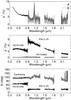 |
Fig. 2 Top: spectroscopic visible (black line) and NIR (gray lines) linear polarization degree of the earthshine obtained on 2013 May 18. Region B (see text) lies spatially near the location of the optical observations; region A includes the Moon terminator. Middle: spectroscopic visible and NIR linear polarization degree of observed polarized and non-polarized standard stars (black lines). Literature photometric polarimetry (Schmidt et al. 1992; Whittet et al. 1992) is plotted as white diamonds, and gray horizontal error bars represent the filter widths. Bottom: spectroscopic polarization vibration angle of the earthshine and polarized standard stars. Symbols are as in previous panels. In all panels, wavelengths strongly affected by telluric absorption are removed. |
The most noticeable feature of the earthshine linear polarization degree is that the polarization intensity is the highest (≥10%) at the bluest wavelengths and steadily decreases toward the red. Various groups (Dollfus 1957; Wolstencroft & Breon 2005; Sterzik et al. 2012; Takahashi et al. 2013; Bazzon et al. 2013) have reported a similar property. In our data, we observe that the linear polarization intensity remains nearly constant at about 5.7% between ~0.8 μm and 0.9 μm. Interestingly, the general shape of the NIR 1−2.3 μm polarimetric spectrum (except for some signatures due to water vapor and oxygen) also appears rather flat within the quoted uncertainties with a value around p∗ = 4.5% independent of wavelength. In contrast, the behavior of the vibration angle appears slightly different. Whereas it remains constant within ± 3° for all optical frequencies, the broad-shaped variations of up to 30° detected in the NIR (which cannot be attributed to instrumental or measurement errors) seem to correlate with the spectral features observed in p∗. This may be attributed to the wavelength-dependent relative contribution of different components (atmospheric species, clouds, aerosols, and surface albedos) to the globally integrated linear polarization of the earthshine.
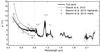 |
Fig. 3 Our visible and NIR spectropolarimetric measurements of the earthshine compared to literature data. A 10-pixel binning was applied to the NIR spectrum of region B. The uncertainty per wavelength is plotted as vertical gray error bars. Wavelengths of strong telluric absorption have been removed. Some molecular species seen in “emission” (indicative of strong atmospheric flux absorption and less multiscattering processes occurring at those particular wavelengths) are labeled. The vertical dashed line separates the ALFOSC and LIRIS data. |
We compare our measurements with data from the literature in Fig. 3. To improve the quality of the NIR linear polarization degree spectrum of region B, we applied a ten-pixel binning in the spectral dimension. Overlaid in Fig. 3 are the optical p∗ values obtained at a spectral resolution of 3 nm and for two separated dates by Sterzik et al. (2012), and the broadband filter measurements of Moon highlands and maria made by Bazzon et al. (2013) for a Sun-Earth-Moon phase angle similar to ours. All optical data display a qualitatively similar pattern (previously discussed), but they differ quantitatively in the amount of polarization per wavelength and the spectral slope. The spectral slope of Sterzik et al. (2012) and Bazzon et al. (2013) data is steeper than the ALFOSC spectrum, while our measurements and those of Takahashi et al. (2013, see their Fig. 3) display related declivity. These differences may be understood in terms of distinct lunar areas explored by the various groups and different observing dates. Sterzik et al. (2012) attributed the discrepancies of their two spectra solely to the time-dependent fraction of Earth clouds, continents, and oceans contributing to the earthshine. Our simultaneous NIR spectra of regions A and B support the conclusion of Bazzon et al. (2013) that linear p∗ values may also partially depend on the exact location of the Moon observed.
Despite the featureless appearance of the polarimetric spectrum of the Earth, some signatures are still observable at the level of ≥3σ and at the resolution and quality of our data. The most prominent molecular features have been identified as labeled in Fig. 3: the optical O2 at 0.760 μm (previously reported by Sterzik et al. 2012), H2O in the intervals 0.653−0.725 μm and 0.780−0.825 μm and the NIR H2O at 0.93 μm and 1.12 μm and O2 at 1.25 μm, the last two reported here for the first time. Linear polarization is higher inside deep absorption molecular bands because strong opacity leaves only upper atmospheric layers to contribute significantly to the observed flux, thus reducing multiple scattered photons with respect to single scattered ones. As discussed by Sengupta (2003) and Stam (2008), single scattering produces more intense polarization indices than multiple scattering events. The presence of the O2A-band at 0.760 μm and H2O at 0.653−0.725 μm, 0.780−0.825 μm, and 0.93 μm in the Earth spectropolarimetry has already been predicted by Stam (2008). These authors stressed the sensitivity of the A-band polarization index to the planetary gas mixing ratio and altitude of the clouds. Interestingly, the peak of the linear polarization at the center of the 1.12-μm H2O band is ~2.7 times greater than the values of the surrounding continuum, i.e., similar in intensity to the blue optical wavelengths. Even more important should be the linear polarization signal of water bands at ~1.4 μm and ~1.9 μm, which unfortunately cannot be characterized from the ground due to strong telluric absorption. Spectropolarimetric models of the Earth, guided by the visible and NIR observations shown here, could provide hints to their expected polarization values.
To this point, we presented earthshine p∗ values as measured from the light deflection on the Moon surface. However, this process introduces significant depolarization due to the back-scattering from the lunar soil (Dollfus 1957); the true linear polarization intensity of the planet Earth is actually higher. At optical wavelengths, the depolarization is estimated at a factor of 3.3λ/550 (λ in nm) by Dollfus (1957), making true polarization fall in the range 26−31%. We are not aware of any determination of the depolarization factor for the NIR in the literature. The extrapolation of Eq. (9) by Bazzon et al. (2013) toward the NIR yields corrections of ~×2.2−×3.3 for the wavelength interval 0.9−2.3 μm, implying that the true linear polarization intensity of the Earth may be ~9−12% for the NIR continuum, and ~12−36% at the peak of the O2 (1.25 μm) and H2O (1.12 μm) bands. The extrapolation of Dollfus (1957) depolarization wavelength dependency toward the NIR would yield even higher true polarization values by a factor of ~4. Further modeling efforts are needed to confirm these features, which may become a powerful tool for the search for Earth-like worlds and their characterization in polarized light.
Ephemeris computations by the Jet Propulsion Laboratory HORIZONS project: http://ssd.jpl.nasa.gov/?horizons
Acknowledgments
This work was based on observations made with the William Herschel and Nordic Optical telescopes operated on the island of La Palma by the Isaac Newton Group and the Nordic Optical Telescope Scientific Association (NOTSA), respectively, in the Spanish Observatorio del Roque de los Muchachos of the Instituto de Astrofísica de Canarias. The instrument ALFOSC is provided by the Instituto de Astrofísica de Andalucía under a joint agreement with the University of Copenhagen and NOTSA. We thank Dr. D. Stam for helpful discussions. This work is partly financed by the Spanish Ministry of Economics and Competitiveness through projects AYA2012-39612-C03-02 and AYA2011-30147-C03-03.
References
- Bazzon, A., Schmid, H. M., & Gisler, D. 2013, A&A, 556, A117 [NASA ADS] [CrossRef] [EDP Sciences] [Google Scholar]
- Cassan, A., Kubas, D., Beaulieu, J.-P., et al. 2012, Nature, 481, 167 [NASA ADS] [CrossRef] [Google Scholar]
- Dollfus, A. 1957, Suppléments aux Annales d’Astrophysique, 4, 3 [NASA ADS] [Google Scholar]
- García Muñoz, A., Zapatero Osorio, M. R., Barrena, R., et al. 2012, ApJ, 755, 103 [NASA ADS] [CrossRef] [Google Scholar]
- Howard, A. W., Marcy, G. W., Bryson, S. T., et al. 2012, ApJS, 201, 15 [NASA ADS] [CrossRef] [Google Scholar]
- Kaltenegger, L., & Traub, W. A. 2009, ApJ, 698, 519 [NASA ADS] [CrossRef] [Google Scholar]
- Karalidi, T., Stam, D. M., & Hovenier, J. W. 2011, A&A, 530, A69 [NASA ADS] [CrossRef] [EDP Sciences] [Google Scholar]
- Manchado, A., Barreto, M., Acosta-Pulido, J., et al. 2004, in Proc. SPIE, 5492, 1094 [Google Scholar]
- Miles-Páez, P. A., Zapatero Osorio, M. R., Pallé, E., & Peña Ramírez, K. 2013, A&A, 556, A125 [NASA ADS] [CrossRef] [EDP Sciences] [Google Scholar]
- Montañés-Rodríguez, P., Pallé, E., Goode, P. R., et al. 2006, ApJ, 651, 544 [NASA ADS] [CrossRef] [Google Scholar]
- Oliva, E. 1997, A&AS, 123, 589 [NASA ADS] [CrossRef] [EDP Sciences] [Google Scholar]
- Pallé, E., Zapatero Osorio, M. R., Barrena, R., et al. 2009, Nature, 459, 814 [NASA ADS] [CrossRef] [PubMed] [Google Scholar]
- Pallé, E., Zapatero Osorio, M. R., & García Muñoz, A. 2011, ApJ, 728, 19 [NASA ADS] [CrossRef] [Google Scholar]
- Schmidt, G. D., Elston, R., & Lupie, O. L. 1992, AJ, 104, 1563 [NASA ADS] [CrossRef] [Google Scholar]
- Sengupta, S. 2003, ApJ, 585, L155 [NASA ADS] [CrossRef] [Google Scholar]
- Stam, D. M. 2008, A&A, 482, 989 [NASA ADS] [CrossRef] [EDP Sciences] [Google Scholar]
- Sterzik, M. F., Bagnulo, S., & Palle, E. 2012, Nature, 483, 64 [NASA ADS] [CrossRef] [Google Scholar]
- Swain, M. R., Vasisht, G., & Tinetti, G. 2008, Nature, 452, 329 [NASA ADS] [CrossRef] [PubMed] [Google Scholar]
- Takahashi, J., Itoh, Y., Akitaya, H., et al. 2013, PASJ, 65, 38 [NASA ADS] [CrossRef] [Google Scholar]
- Turnbull, M. C., Traub, W. A., Jucks, K. W., et al. 2006, ApJ, 644, 551 [NASA ADS] [CrossRef] [Google Scholar]
- Wardle, J. F. C., & Kronberg, P. P. 1974, ApJ, 194, 249 [NASA ADS] [CrossRef] [Google Scholar]
- Whittet, D. C. B., Martin, P. G., Hough, J. H., et al. 1992, ApJ, 386, 562 [NASA ADS] [CrossRef] [Google Scholar]
- Wolstencroft, R. D., & Breon, F.-M. 2005, in ASP Conf. Ser., 343, 211 [Google Scholar]
- Woolf, N. J., Smith, P. S., Traub, W. A., & Jucks, K. W. 2002, ApJ, 574, 430 [NASA ADS] [CrossRef] [Google Scholar]
- Zapatero Osorio, M. R., Caballero, J. A., & Béjar, V. J. S. 2005, ApJ, 621, 445 [NASA ADS] [CrossRef] [Google Scholar]
- Zapatero Osorio, M. R., Béjar, V. J. S., Goldman, B., et al. 2011, ApJ, 740, 4 [NASA ADS] [CrossRef] [Google Scholar]
All Tables
All Figures
|
Fig. 1 Relative positions of the ALFOSC and LIRIS slits on the Moon surface during the observations of the lunar nightside on 2013 May 18. Equatorial coordinates α and δ correspond to 21h20m universal time. For displaying purposes, the slit widths are multiplied by a factor of four, and the slit lengths are plotted on true scale. |
| In the text | |
|
Fig. 2 Top: spectroscopic visible (black line) and NIR (gray lines) linear polarization degree of the earthshine obtained on 2013 May 18. Region B (see text) lies spatially near the location of the optical observations; region A includes the Moon terminator. Middle: spectroscopic visible and NIR linear polarization degree of observed polarized and non-polarized standard stars (black lines). Literature photometric polarimetry (Schmidt et al. 1992; Whittet et al. 1992) is plotted as white diamonds, and gray horizontal error bars represent the filter widths. Bottom: spectroscopic polarization vibration angle of the earthshine and polarized standard stars. Symbols are as in previous panels. In all panels, wavelengths strongly affected by telluric absorption are removed. |
| In the text | |
|
Fig. 3 Our visible and NIR spectropolarimetric measurements of the earthshine compared to literature data. A 10-pixel binning was applied to the NIR spectrum of region B. The uncertainty per wavelength is plotted as vertical gray error bars. Wavelengths of strong telluric absorption have been removed. Some molecular species seen in “emission” (indicative of strong atmospheric flux absorption and less multiscattering processes occurring at those particular wavelengths) are labeled. The vertical dashed line separates the ALFOSC and LIRIS data. |
| In the text | |
Current usage metrics show cumulative count of Article Views (full-text article views including HTML views, PDF and ePub downloads, according to the available data) and Abstracts Views on Vision4Press platform.
Data correspond to usage on the plateform after 2015. The current usage metrics is available 48-96 hours after online publication and is updated daily on week days.
Initial download of the metrics may take a while.