| Issue |
A&A
Volume 562, February 2014
|
|
|---|---|---|
| Article Number | A116 | |
| Number of page(s) | 8 | |
| Section | Planets and planetary systems | |
| DOI | https://doi.org/10.1051/0004-6361/201322933 | |
| Published online | 17 February 2014 | |
Stellar wind interaction and pick-up ion escape of the Kepler-11 “super-Earths”
1
Space Research Institute, Austrian Academy of Sciences,
Schmiedlstrasse 6,
8042
Graz,
Austria
2
University of Vienna, Department of Astrophysics,
Türkenschanzstrasse 17,
1180
Wien,
Austria
3
Institute of Physics, University of Graz, Universitätsplatz 5,
8010
Graz,
Austria
4
Institute of Computational Modelling, Siberian Division of Russian
Academy of Sciences, 660036
Krasnoyarsk, Russian
Federation
5
Siberian Federal University, Krasnoyarsk, Russian
Federation
6
Swedish Institute of Space Physics, Box 812, 98128
Kiruna,
Sweden
7
Institute of Nuclear Physics, Moscow State University,
Leninskie Gory,
119992
Moscow,
Russia
Received:
29
October
2013
Accepted:
16
December
2013
Abstract
Aims. We study the interactions between stellar winds and the extended hydrogen-dominated upper atmospheres of planets. We estimate the resulting escape of planetary pick-up ions from the five “super-Earths” in the compact Kepler-11 system and compare the escape rates with the efficiency of the thermal escape of neutral hydrogen atoms.
Methods. Assuming the stellar wind of Kepler-11 is similar to the solar wind, we use a polytropic 1D hydrodynamic wind model to estimate the wind properties at the planetary orbits. We apply a direct simulation Monte Carlo model to model the hydrogen coronae and the stellar wind plasma interaction around Kepler-11b–f within a realistic expected heating efficiency range of 15–40%. The same model is used to estimate the ion pick-up escape from the XUV heated and hydrodynamically extended upper atmospheres of Kepler-11b–f. From the interaction model, we study the influence of possible magnetic moments, calculate the charge exchange and photoionization production rates of planetary ions, and estimate the loss rates of pick-up H+ ions for all five planets. We compare the results between the five “super-Earths” and the thermal escape rates of the neutral planetary hydrogen atoms.
Results. Our results show that a huge neutral hydrogen corona is formed around the planet for all Kepler-11b–f exoplanets. The non-symmetric form of the corona changes from planet to planet and is defined mostly by radiation pressure and gravitational effects. Non-thermal escape rates of pick-up ionized hydrogen atoms for Kepler-11 “super-Earths” vary between ~6.4 × 1030 s-1 and ~4.1 × 1031 s-1, depending on the planet’s orbital location and assumed heating efficiency. These values correspond to non-thermal mass loss rates of ~1.07 × 10⁷ g s-1 and ~6.8 × 10⁷ g s-1 respectively, which is a few percent of the thermal escape rates.
Key words: planet-star interactions / planets and satellites: atmospheres / planets and satellites: individual: Kepler-11 system / methods: numerical
© ESO, 2014
1. Introduction
Due to progress in ground-based radial velocity surveys and the two space observatories, CoRoT and Kepler, an increasing number of transiting exoplanets in the “super-Earth” domain with radii between ~1.5−3 R⊕ and masses that are ≤10 M⊕ have been discovered. If one compares the average densities of these exoplanets to that of the Earth, one finds that the size of several “super-Earths” is too large to have Earth-type compositions. Only “super-Earths” orbiting their host stars at distances below 0.05 AU, such as CoRoT-7b (Léger et al. 2009), Kepler-10b (Batalha et al. 2011), and Kepler-18b (Cochran et al. 2011), show radius-mass related average densities that agree with pure rocky bodies without gaseous envelopes. This radius-mass anomaly indicates that the majority of each of these exoplanets contains a huge fraction of their primordial nebula-based hydrogen-dominated protoatmospheres or volatile materials, such as evaporated ices and hydrogen-rich H2O, CH4, and NH3. The result that such volatile-rich exoplanets should exist in the inner regions of exosolar planetary systems was predicted nearly a decade ago by Kuchner (2003) and Léger et al. (2004). In this context, it is interesting that the compact “super-Earths” of the Kepler-11 system, Kepler-11d, Kepler-11e, and Kepler-11f, are most likely to contain large volumes of hydrogen, while Kepler-11b and Kepler-11c may be rich in ices similar to Uranus and Neptune surrounded by a H/He mixture (Lissauer et al. 2011).
Planetary and stellar parameters for the Kepler-11 system given in Earth masses and radii.
Recently, Lammer et al. (2013) studied the non-hydrostatic upper atmosphere structure and blow-off criteria of seven “super-Earths” with known sizes and masses, which included Kepler-11b–f. By assuming that the thermospheres of these planets are dominated by hydrogen, the results of this study indicate that their upper atmospheres may expand to several planetary radii and, with the exception of Kepler-11c, have exobase levels that extend beyond the Roche lobe, indicating that they all experience atmospheric mass-loss due to Roche lobe overflow (e.g., Lecavelier des Etangs et al. 2004; Erkaev et al. 2007). Lammer et al. (2013) found that the atmospheric mass loss of the studied “super-Earths” is one to two orders of magnitude lower compared to that of “hot Jupiters”, such as HD 209458b, so that one can expect that these exoplanets cannot lose their present hydrogen envelopes via thermal escape during their remaining lifetimes.
Because the upper atmospheres of these planets can expand to large distances, one can assume that huge extended hydrogen coronae should form around the planets above a possible magnetopause obstacle, so that planetary atoms can directly interact with the stellar wind plasma. This results in non-thermal ion pick-up escape.
The aim of this study is to investigate the expected hydrogen coronae around these five “super-Earths” within the Kepler-11 system, the stellar wind, and XUV induced H+ pick-up ion escape rates and to compare their efficiency with the thermal loss rates given in Lammer et al. (2013). For the first time, this study allows us to obtain an estimate of the thermal and non-thermal ion pick-up escape rates from observed “super-Earths”, which are located in different orbital distances inside the same planetary system. Table 1 summarizes the parameters of the Kepler-11 system. For Kepler-11, the distance between this star and the Sun is given. In the present study, we do not consider Kepler-11g which is a Jupiter-type gas giant.
We apply a direct simulation Monte Carlo (DSMC) exosphere-stellar wind plasma interaction model (Holmström et al. 2008; Ekenbäck et al. 2010; Kislyakova et al. 2013) to the soft X-ray and extreme ultraviolet (XUV) heated and dynamically expanded upper atmospheres of Kepler-11b–f. In Sect. 2, we describe the radiation, expected stellar wind plasma parameters, and the magnetic properties of the host star. In Sect. 3, we briefly describe the DSMC model, which is used for the calculation of the hydrogen coronae and the coupled solar/stellar wind plasma model. We also briefly address possible planetary obstacles and expected magnetospheres of these planets. In Sect. 4, we calculate the ion production rates and estimate the resulting ion pick-up escape and mass loss rates. Finally, we compare the H+ ion pick-up escape rates with the thermal escape rates of the neutral hydrogen atoms.
2. Radiation and stellar wind properties
2.1. Estimated XUV and Lyα emission of Kepler-11
Stellar input parameters at the orbital locations of Kepler-11b-f.
Kepler-11 is a slightly evolved, solar-like G-star with a radius Rst of 1.1 ± 0.1 RSun and a mass Mst of 0.95 ± 0.1 MSun (Lissauer et al. 2011). At present, the X-ray and EUV (XUV) emission of Kepler-11 is observationally unconstrained. This is mainly due to its large distance of several hundred parsecs and its old age (6−10 Gyr; Lissauer et al. 2011), which implies a low level of activity. Therefore, we adopt the XUV fluxes at the respective planetary orbits given in Lammer et al. (2013), which are based on power laws derived from observations of nearby solar-like stars of different ages (Ribas et al. 2005). At the orbits of Kepler-11b–f, the XUV fluxes are enhanced by factors IXUV of 60, 45, 20, 13, and 8 (cf. Table 2) over the average present solar XUV flux at 1 AU (4.64 erg cm-2 s-1; Ribas et al. 2005). Note that the uncertainties in IXUV might be up to an order of magnitude because of the lack of relevant observations and weak constraints on the age or activity level of the host star Kepler-11 (Lammer et al. 2013). The enhancement factors are used to calculate the photoionization rates, which are needed as input for the DSMC ENA model presented here. The mean photoionization rate of 1.1 × 10⁻⁷ s-1 at the present Earth (e.g., Bzowski 2008) is scaled up by IXUV and corresponds to τpi values for planets Kepler-11b–f given in Table 2.
Another required model input parameter is the UV absorption rate, which is defined as βabs = ∫σ(λ)Φ(λ)dλ, where σ(λ) is the absorption cross-section and Φ(λ) is the stellar Lyα spectrum (e.g. Meier 1995). The absorption cross-section is σ(λ) = ∫ψ(v)σN(λ′)dv, where ψ(v) is the normalized atomic velocity distribution and σN(λ′) is the natural absorption cross-section of an atom traveling with velocity v for which λ′ = λ(1 − v/c). When the atomic velocities are very small, the UV absorption rate can be approximated by the product of the total cross-section at Lyα, σLyα = ∫σ(λ)dλ = 5.47 × 10⁻¹⁵ cm2 Å (e.g. Quémerais 2006), and the stellar Lyα photon flux at the line center. If we estimate the central Lyα flux of Kepler-11 using a scaling law from Ribas et al. (2005) for the total line flux as a function of stellar age and divide it by the effective line width (~1 Å; Meier 1995), we obtain the UV absorption rates βabs for Kepler-11b–f given in Table 2.
The UV absorption rates might deviate from the values given above, especially for atoms with high radial velocities. Therefore, we calculate a velocity-dependent UV absorption rate. For this, we need the intrinsic (unabsorbed) stellar Lyα line profile, which is not available for Kepler-11. Hence, we adopt the reconstructed intrinsic Lyα profile of the Sun-like star 61 Vir presented in Wood et al. (2005). This G5V star is located at a distance of approximately 8.5 pc and has an estimated age range of 6−12 Gyr (Vogt et al. 2010). Despite very similar masses, 61 Vir appears to be smaller than Kepler-11, indicating that it is probably younger. However, since it has the weakest intrinsic Lyα emission observed from Sun-like stars to date (Linsky et al. 2013), we adopt its profile as a proxy for to profile of Kepler-11. To obtain the Lyα fluxes at the orbits of the Kepler-11 planets, we scale the apparent intrinsic flux of 61 Vir (Wood et al. 2005) according to the star’s distance (8.555 pc; Linsky et al. 2013) and the orbital distances of the Kepler-11 planets (cf. Table 1). The line profile has also been shifted in wavelength to account for the radial velocity of 61 Vir (−8.1 km s-1; Kharchenko et al. 2007).
We define the velocity-dependent UV absorption rate per atom β(v) such
that βabs = ∫ψ(v)β(v)dv.
Therefore,  , as can be derived from the
equations given above. Because the natural absorption cross-section is very narrow
compared to the stellar line profile, it can be approximated by a delta function;
therefore,
, as can be derived from the
equations given above. Because the natural absorption cross-section is very narrow
compared to the stellar line profile, it can be approximated by a delta function;
therefore,  , where λ0 = 1215.67 Å
is the central wavelength of Lyα. The resulting absorption rates at the orbits of
Kepler-11b–f as a function of atomic radial velocity are shown in Fig. 1. We define velocities in the direction of the star to
be positive. Note that the values found in the line center, i.e. for atoms with
v ≈ 0, are
in good agreement with the simple calculations given in Table 2. However, we use the rates shown in Fig. 1 in the DSMC simulations presented below for better accuracy.
, where λ0 = 1215.67 Å
is the central wavelength of Lyα. The resulting absorption rates at the orbits of
Kepler-11b–f as a function of atomic radial velocity are shown in Fig. 1. We define velocities in the direction of the star to
be positive. Note that the values found in the line center, i.e. for atoms with
v ≈ 0, are
in good agreement with the simple calculations given in Table 2. However, we use the rates shown in Fig. 1 in the DSMC simulations presented below for better accuracy.
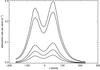 |
Fig. 1 Kepler-11 Lyα absorption rate as a function of neutral hydrogen radial velocity. The lines from top to bottom correspond to the orbit locations of Kepler-11b–f. |
2.2. Expected stellar wind plasma properties
In this section, we estimate stellar wind speeds, densities, temperatures, and magnetic field strengths at the planetary orbital locations. Since the properties of the winds of low-mass stars are unconstrained by both theory and observation, we assume that the stellar wind of Kepler-11 is similar to the solar wind. This is a reasonable assumption, given the similarities between Kepler-11 and the Sun.
We apply a 1D hydrodynamic model for the solar wind propagation by using the publicly available MHD code Nirvana (Ziegler 2005). We assume that the wind is driven by thermal pressure gradients. In this model, the acceleration of the wind is governed by the amount and distribution of heating that is given to the wind. Since the heating mechanisms are unknown, we implicitly heat the wind by assuming a polytropic equation of state, where the pressure is assumed to be proportional to the mass density to the power of a polytropic index α, thus giving p = Kρα (this is equivalent to assuming that the temperature is given by Tsw ∝ ργ−1). This assumption means that we do not solve the energy equation in our hydrodynamic simulation. Assuming radial variations in the values of K and α, Jacobs & Poedts (2011) produced a series of 1D models for the solar wind that reproduces a range of slow and fast solar wind properties at 1AU as measured by the ACE satellite. We reproduce one of their models that gives typical slow solar wind properties at 1 AU. Given that the planets are likely to orbit close to the stellar equatorial plane (cf. Table 1), by analogy with the Sun, it is reasonable to assume that they experience mostly slow solar wind conditions, which dominate in the equatorial plane throughout most of the solar cycle for the solar wind (Ebert et al. 2009). In this model, we assume a particle number density at the base of the wind of 7.0 × 108 cm-3 and a temperature of 1.625 × 10⁶ K. The α parameter varies smoothly from a value of 1.22 near the stellar surface to 1.42 at 23 Rst and is then uniform out to 1 AU. This leads to a wind proton density of 5.3 protons cm-3 and a temperature of 1.3 × 10⁵ K at 1 AU. These are reasonable values for the slow solar wind, as measured by the ACE satellite (e.g. Wargelin et al. 2004; Vršnak et al. 2007; Manoharan 2012). The mass density, velocity, and pressure of the wind as a function of radial distance from the star are shown in Fig. 2.
To estimate the strength of the stellar magnetic field far from the star, it is necessary
to know the strength of the dipole component of the field close to the star. Since there
exists no measurements of the strength of Kepler-11’s magnetic field, we scale the
strength of the solar dipole to Kepler-11 using the rotation-activity relation given by
Saar (1996) of
 .
We estimate the rotation period of Kepler-11 using its age and the rotation-age relation
of log (1/Prot) = 1.865−2.254t0.083
given by Guinan & Engle (2009), where
Prot is the rotation period in days and
t is the
stellar age in Gyr. This gives a rotation period for Kepler-11 of 33.5 days, and assuming
that the inclination angle of the axis-of-rotation is 90°, this corresponds to a
projected rotational velocity at the equator of 1.66 km s-1. We check that this value is
reasonable by computing an atmospheric model using LLmodels (Shulyak et al. 2004) and calculating synthetic spectra
with synth3 (Kochukhov 2007), which we then compare
to spectroscopic observations obtained with the Keck I telescope and de-archived from Keck
Observatory Archive (KOA). The basic physical parameters of the star, Teff = 5680 K
± 100 K and log g = 4.3 ± 0.2 are
adopted from Lissauer et al. (2013). The atomic
data used for spectrum synthesis is extracted from the Vienna Atomic Line Database (VALD,
Piskunov et al. 1995; Ryabchikova et al. 1999; Kupka et al.
1999). Comparing the synthetic spectra to selected suitable spectral lines from
the Keck I observations, we get an estimate for the projected rotational velocity of
Kepler-11 of 1.5 ± 1 km s
-1, which is
similar to the value calculated above. Assuming a dipole field strength of 5 G for the
Sun, we get a dipole field strength of 3.5 G for Kepler-11.
.
We estimate the rotation period of Kepler-11 using its age and the rotation-age relation
of log (1/Prot) = 1.865−2.254t0.083
given by Guinan & Engle (2009), where
Prot is the rotation period in days and
t is the
stellar age in Gyr. This gives a rotation period for Kepler-11 of 33.5 days, and assuming
that the inclination angle of the axis-of-rotation is 90°, this corresponds to a
projected rotational velocity at the equator of 1.66 km s-1. We check that this value is
reasonable by computing an atmospheric model using LLmodels (Shulyak et al. 2004) and calculating synthetic spectra
with synth3 (Kochukhov 2007), which we then compare
to spectroscopic observations obtained with the Keck I telescope and de-archived from Keck
Observatory Archive (KOA). The basic physical parameters of the star, Teff = 5680 K
± 100 K and log g = 4.3 ± 0.2 are
adopted from Lissauer et al. (2013). The atomic
data used for spectrum synthesis is extracted from the Vienna Atomic Line Database (VALD,
Piskunov et al. 1995; Ryabchikova et al. 1999; Kupka et al.
1999). Comparing the synthetic spectra to selected suitable spectral lines from
the Keck I observations, we get an estimate for the projected rotational velocity of
Kepler-11 of 1.5 ± 1 km s
-1, which is
similar to the value calculated above. Assuming a dipole field strength of 5 G for the
Sun, we get a dipole field strength of 3.5 G for Kepler-11.
For the radial dependence of the strength of the dipole component, we assume that the field decreases as a dipole (i.e. B ∝ r-3) out to the source-surface, where the coronal plasma pressure dominates the magnetic pressure and forces the magnetic field lines open. Outside of the source-surface, we assume that the field falls off as a radial field (i.e. B ∝ r-2). Based on the solar analogy, we take the source-surface to be at 2.5 Rst. This model gives a value of 4.3 nT at 1 AU for the solar case, and the field strengths at each planetary orbital distance for Kepler-11 planets are given in Table 2.
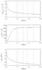 |
Fig. 2 Modeled stellar wind parameters (nsw, vsw, psw) as a function of orbital distance. The dashed lines correspond to the orbit locations of Kepler-11b–f. |
3. Upper atmosphere and stellar wind interaction modeling
3.1. Method
We study the plasma interactions between the stellar wind of Kepler-11 and the upper atmospheres of the Kepler-11 “super-Earths” by applying a DSMC upper atmosphere-exosphere 3D particle model. The software is based on the FLASH code written in Fortran 90, which is publicly available (Fryxell et al. 2000). The code follows particles in the simulation domain according to all forces acting on a hydrogen atom and includes two species: neutral hydrogen atoms and hydrogen ions (which also include stellar wind protons). The application of the FLASH code to the physics of upper planetary atmospheres is described in detail in Holmström et al. (2008), Ekenbäck et al. (2010), and Kislyakova et al. (2013). The model includes the following processes/forces, which may act on an exospheric atom:
-
1.
Collision with an UV photon, which can occur if the particle is outside of the planet’s shadow, which leads to an acceleration of the hydrogen atom away from the star. As in Holmström et al. (2008) and Ekenbäck et al. (2010) an UV photon is absorbed by a neutral hydrogen atom, leading to a radial velocity change and then consequently reradiated in a random direction. However, in the present study, the UV collision rate is velocity dependent, as shown in Fig. 1.
-
2.
Photoionization by a stellar photon or a stellar wind electron impact ionization. The rates, τpi and τei, are presented in Table 2, and τei is taken according to Holzer (1977). Estimation of the photoionization rate τpi is described in Sect. 2.1. We do not include ionization by the atmospheric electrons, because the electron ionization rate strongly depends on the electron temperature and is very low for the atmospheric values of Tel (Holzer 1977).
-
3.
Charge exchange between neutral hydrogen atoms and stellar wind protons. If a hydrogen atom is outside the planetary obstacle (magnetopause, or ionopause) it can undergo charge exchange with a stellar wind proton, producing an energetic neutral atom (ENA). The charge exchange cross-section is taken to be equal to 2 × 10-19 m2 (Lindsay & Stebbings 2005).
-
4.
Elastic collision with another hydrogen atom. Here the collision cross-section was taken to be 10-21 m2 (Izmodenov et al. 2000).
Collisions with cold H+ of planetary origin are not taken into account. These ions are abundant in particular at the border of the planetary obstacle, but they should not alter the results significantly. Although the cross-section is large for low velocity H-H+ (Lindsay & Stebbings 2005), neutral H dominates at low energies by orders of magnitudes (in our model), so the effect of charge exchange should be minimal at low energies.
The coordinate system is centered at the center of the planet with the x-axis pointing towards the center of mass of the system, the y-axis pointing in the direction opposite to the planetary motion, and the z-axis pointing parallel to the vector Ω that represents the orbital angular velocity of the planet around the central star. The Mst is the mass of the planet’s host star. The outer boundary of the simulation domain is the box xmin ≤ x ≤ xmax, ymin ≤ y ≤ ymax, and zmin ≤ z ≤ zmax. The inner boundary is a sphere of radius R0.
We obtain the planetary input parameters, such as density, temperature, and bulk outflow velocity of the upper atmosphere, for the inner boundary in the 3D DSMC particle code in the same way as described in detail in Lammer et al. (2013). Our assumed lower thermospheric conditions are also similar to those assumed in Lammer et al. (2013). We used the time-dependent numerical algorithm which solves the 1D fluid equations for mass, momentum, and energy conservation from the base of the thermosphere until the height R0 where the Knudsen number Kn is 0.1 (Johnson et al. 2013). The Knudsen number is the ratio of the mean free path to the corresponding scale height, and the exobase is defined as the surface where Kn = 1. Using kinetic 3D modeling above R0 is more accurate because, as we show, the hydrogen coronae are strongly deformed by the radiation pressure for the Kepler-11 planets.
Tidal potential, Coriolis force and centrifugal force, and the gravitation of the star
and planet, which act on a hydrogen neutral atom are included in the following way (after
Chandrasekhar 1963): ![Mathematical equation: \begin{eqnarray} \label{e_SCG} \frac{{\rm d} v_{\rm i}}{{\rm d}t}&=&\frac{\partial}{\partial x_{\rm i}} \left[ \frac{1}{2}\Omega^2 \left(x_1^2+x_2^2 \right)+ \mu\left(x_1^2-\frac{1}{2}x_2^2 -\frac{1}{2}x_3^2 \right)\right. \nonumber \\ &&\left. +\left(\frac{G M_{\rm st}}{R^2}-\frac{M_{\rm st} R}{M_{\rm pl} + M_{\rm st}}\Omega^2 \right)x_1 \right] + 2\Omega \epsilon_{\rm il3} v_{\rm l} \end{eqnarray}](/articles/aa/full_html/2014/02/aa22933-13/aa22933-13-eq125.png) (1)Here
x1 = x, x2 = y, x3 = z, and
vi are the components of the velocity
vector of a particle; G is Newton’s gravitational constant; R is the distance between
the centers of mass; ϵilk is the Levi-Civita symbol; and
μ is given
by μ = GMst/R3.
The first term in the right-hand side of Eq. (1) represents the centrifugal force, and the second is the tidal-generating
potential; the third corresponds to the gravitation of the planet’s host star and the
planet, while the last term stands for the Coriolis force. The self-gravitational
potential of the particles is neglected.
(1)Here
x1 = x, x2 = y, x3 = z, and
vi are the components of the velocity
vector of a particle; G is Newton’s gravitational constant; R is the distance between
the centers of mass; ϵilk is the Levi-Civita symbol; and
μ is given
by μ = GMst/R3.
The first term in the right-hand side of Eq. (1) represents the centrifugal force, and the second is the tidal-generating
potential; the third corresponds to the gravitation of the planet’s host star and the
planet, while the last term stands for the Coriolis force. The self-gravitational
potential of the particles is neglected.
3.2. Possible planetary obstacles
Charge exchange reactions between stellar wind protons and neutral planetary particles
consist of the transfer of an electron from a neutral atom to a proton that leaves a cold
atmospheric ion and an energetic neutral atom. This process is described by the following
reaction:  . After its
production, an ENA continues to travel with the initial velocity and energy of the stellar
wind proton. The atmospheric atom becomes an initially cold ion, which can afterwards be
lost from the atmosphere due to the ion pick-up process (see Sect. 4).
. After its
production, an ENA continues to travel with the initial velocity and energy of the stellar
wind proton. The atmospheric atom becomes an initially cold ion, which can afterwards be
lost from the atmosphere due to the ion pick-up process (see Sect. 4).
Charge exchange takes place outside of an obstacle that corresponds to the magnetopause
or ionopause boundary, which we assume is a surface described by:  (2)
(2)
where Rs is the substellar point of the obstacle and Rt is the obstacle width at the planetary terminator. Changing these two parameters, one may model various types of the interaction, such as the interaction between the stellar wind and a magnetized or non-magnetized body. More details are given in Kislyakova et al. (2013). The obstacle is rotated by an angle of arctan(vp/vsw) to account for the finite stellar wind speed relative to the planet’s orbital speed. The protons do not penetrate a magnetic obstacle.
For magnetized planets, the dynamical pressure of the stellar wind is balanced by the pressure of the atmosphere together with the magnetic pressure defined by the intrinsic magnetic moment of the planet. Types of expected magnetospheres of exoplanets were considered in detail, for example, by Khodachenko et al. (2012). Because the magnetic fields of the Kepler-11 planets are unknown, we focus on non-magnetized planets without additional magnetic protection by intrinsic dynamos or magnetic discs in the present study (Khodachenko et al. 2012). Under this assumption, the dynamic pressure of the Kepler-11 wind can be balanced by the weak atmospheric pressure in the upper layers of the atmospheres of Kepler-11b–f only very close to R0. For simplicity, we do not consider the magnetic pressure from induced currents in the ionosphere. Since the hydrogen coronae around the planets are not symmetric (see the following section), this moves the interaction boundary close to the planet. In our simulations, we assume Rs to be slightly above R0 and Rs = Rt, which corresponds to a Venus-type narrow magnetic obstacle. Magnetically non-protected planets undergo the strongest interaction processes. Thus, this approach allows us to estimate the highest possible pick-up escape rates.
3.3. Hydrogen coronae and modeling results
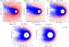 |
Fig. 3 Slices of modeled 3D atomic hydrogen coronae around the five Kepler-11 “super-Earths” for −107 ≤ z ≤ 107 m with a heating efficiency η = 15%. Blue and red dots correspond to neutral hydrogen atoms and hydrogen ions, which include stellar wind protons, respectively. The black dot in the center represents the planet. The white empty area around the planet corresponds to the XUV heated, hydrodynamically expanding thermosphere up to the height R0, where Kn = 0.1. |
Planetary and upper atmosphere input parameters at the height R0 η = 15%,η = 40% where the Kn = 0.1, as the starting point for the DSMC-code simulations for two heating efficiencies η = 15% and 40%.
In this section, we present the results of the modeled hydrogen clouds around the five Kepler-11 “super-Earths”. Huge coronae of neutral hydrogen are formed around each of these low density “super-Earths”. Figure 3 illustrates the appearance of the hydrogen coronae near the planets for a heating efficiency, η, of 15%. The heating efficiency corresponds to the ratio of the absorbed XUV energy that is transferred into heat of the neutral gas. Values of 15% and 40% are considered to be the most realistic (see discussion in Chassefière 1996; Erkaev et al. 2013; Lammer et al. 2013). The atmospheric input parameters are given in Table 3. In Table 3, R0 corresponds to the simulation starting level given in planetary radii, and n and T stand for the atmospheric density and temperature at the same height. Finally, vflow denotes the bulk outflow velocity at R0, which is caused by the strong XUV heating of the atmosphere and the resulting hydrodynamic expansion (see Lammer et al. 2013). All parameters are given for both η = 15% and 40%. Stellar wind and radiation input parameters are described above in Sect. 2 and can be found in Tables 1 and 2 together with planetary masses and radii.
As one can see from Fig. 3, the hydrogen coronae around the Kepler-11 planets strongly deviate from the spherically symmetric form assumed by Lammer et al. (2013), where radiation pressure effects were not taken into account. There are several reasons for the modifications of the shapes of the coronae: first, the radiation pressure from Kepler-11 accelerates the neutral atoms that are outside the optical shadow of the planet away from the star, which leads to the formation of a cometary-like tail bent by the Coriolis force; second, charge-exchange and electron impact ionization reduce the neutral hydrogen density outside the magnetic obstacle. Third, the tidal force leads to the deformation of the cloud. Although these effects for these planets are not so strong in comparison to “Hot Jupiters”, such as HD 209458b or HD 189733b (Bourrier & Lecavelier des Etangs 2013), they are of significant importance. Unlike electron impact ionization, photoionization can also occur inside the planetary obstacle but only outside the optical shadow. The hydrogen atoms that have undergone charge-exchange are identified by an enhanced H+ density near the interaction border along the planetary obstacle.
The high radiation pressure of Kepler-11 and gravitational effects lead to the formation of non-symmetric tails on both sides of a planet in any given plane. In 3D, these tails correspond to a non-symmetric ring of accelerated neutral hydrogen atoms. For a heating efficiency of 40%, the atmospheres are slightly more inflated, but the coronae do not differ much qualitatively from those shown in Fig. 3. One can also see that planets in orbital locations further from their host star, where either radiation pressure or tidal forces are weaker, have hydrogen coronae that differ only slightly from spherical forms (Kislyakova et al. 2013). However, these effects cannot be neglected in the case of close-in exoplanets.
It should be mentioned that the so-called self-shielding effect in some cases can significantly diminish the acceleration by radiation pressure and photoionization of neutral hydrogen atoms (Bourrier & Lecavelier des Etangs 2013), and decrease the length of the accelerated neutral hydrogen tail behind the planet. Self-shielding means that the medium becomes optically thick in Lyα, which prevents the UV photons from penetrating inside the deeper layers and interacting with hydrogen atoms. In the present study, we do not include either UV scattering or photoionization in atmospheres below R0, which are protected from the UV radiation by the upper atmosphere. For the hot gas giants considered by Bourrier & Lecavelier des Etangs (2013), self-shielding is also important in the exosphere, but one should note that the hydrogen density in the upper atmosphere of a “Hot Jupiter” exceeds the upper atmosphere densities of the Kepler-11 “super-Earths” by approximately two orders of magnitude. For this reason, we do not include self-shielding effects into the DSMC upper atmosphere modeling presented in the current study.
4. Ion production and pick-up escape
In this section, we present our estimate of the ion production rates for Kepler-11b–f. These estimations are obtained in the same way as described in detail by Kislyakova et al. (2013). Therefore, we only briefly summarize the main aspects in this study.
Ion production rates, thermal escape rates, and H+ gyro radii for Kepler-11 planets.
In the hydrogen-rich upper atmospheres of the five studied Kepler-11 planets, the H+ ions of planetary origin are produced by charge-exchange reactions, photoionization and electron impact ionization processes. The intensity of the interactions and the number of ions produced vary from planet to planet and depend on upper planetary density and stellar wind parameters, which are functions of orbital distance for a particular star. Planetary obstacles and hydrogen coronae shapes also play a role. While we assume all Kepler-11 “super-Earths” are non-magnetized and have narrow magnetopauses/ionopauses close to the planets, the forms of the clouds are mostly defined by radiation pressure and charge-exchange and differ significantly from planet to planet (Fig. 3). Strong radiation pressure accelerates neutral hydrogen atoms and moves them away from the planet, where they may undergo either charge-exchange or ionization by stellar XUV radiation or by stellar wind electrons easier.
Average ion production rates, Lion, which depend on coronal conditions related to heating efficiency are presented in Table 4. Ion production and thermal loss rates are given in particles per second and mass loss rates are given in grams per second. Estimations of hydrogen thermal loss rates, Lth, shown in the same table are taken from Table 3 of Lammer et al. (2013). Thermal losses given in Lammer et al. (2013) present the calculation of losses from the whole atmosphere and start from the inner boundary of the simulation domain, which is well below Lagrange point L1. In this paper, authors calculate how many particles can reach the L1 point and are lost if the planet undergoes various levels of XUV heating. In the present paper, however, we consider ion-pickup, which is a separate loss mechanism. It is a nonthermal mechanism, when particles do not obtain energy from thermal heating, but are accelerated and swept away from the planet by the stellar wind. An ion can be lost everywhere outside the magnetosphere/ionosphere of a planet. This mechanism has been observed to be effective for present-day Mars and Venus (see for example Lundin 2011). Their atmospheres also do not extend beyond the L1 point. For this reason, the main atmospheres of Kepler-11 exoplanets also should not fill the whole Roche lobe to experience nonthermal ion pickup escape, and one can calculate pickup losses starting from the magnetic boundary, as we do below.
As can be seen in Table 4, the heating efficiency, η, also influences interactions between stellar winds and upper atmospheres. Higher values for η result in higher ion production rates. As a consequence of a higher heating efficiency (40% in considered case), the upper atmospheres expand more, which intensifies the stellar wind interaction processes. The corresponding stellar wind parameters (velocity, density, temperature) are discussed in Sect. 2.2 and can be found in Table 2.
Ions produced beyond the planetary obstacle can be lost because of the ion pick-up process.
Since these particles are no longer neutral, they are forced to follow the stellar wind
plasma flow, detach from the planet, and finally escape from its gravity field. We consider
the H+ ions produced
above the planetary obstacle, where the collisions between atmospheric particles can be
neglected (although we start at Kn = 0.1, radiation pressure reshapes the exosphere
and makes the hydrogen density drop off more rapidly on the starward side compared to the
nondisturbed case). The presence of collisions would reduce the ion pickup escape and not
change the main conclusion of the article, in which the nonthermal ion pickup is smaller
compared to the thermal losses for exoplanets considered here. Taking into account the
interplanetary magnetic field in the vicinity of the planets (see Table 2), we can calculate the gyro radius for H+:
 (3)where mH,
v, and
q are the
mass, velocity and electric charge of a hydrogen ion, B is the stellar magnetic
field near the planet, and kB is the Boltzmann constant. We calculate
two values of rg,
(3)where mH,
v, and
q are the
mass, velocity and electric charge of a hydrogen ion, B is the stellar magnetic
field near the planet, and kB is the Boltzmann constant. We calculate
two values of rg,  corresponds
to the “cold” ions and
corresponds
to the “cold” ions and  corresponds to
ions that are accelerated by the electric fields in the stellar wind until they reach the
speed of the stellar wind in the vicinity of the planet (Lundin 2011). The “cold” ion velocity is taken to equal the most probable
Maxwellian speed
corresponds to
ions that are accelerated by the electric fields in the stellar wind until they reach the
speed of the stellar wind in the vicinity of the planet (Lundin 2011). The “cold” ion velocity is taken to equal the most probable
Maxwellian speed  km s-1 for T = 400 K, which is the
lowest temperature used in the simulations. As in Kislyakova
et al. (2013), we assume that an ion is lost from the planet if its gyro radius
does not exceed R0. This means that the magnetic field can
significantly influence the trajectory of the particles. As can be seen in Table 4, the gyro radius of H+ ions is several orders of
magnitude smaller than the planetary radius even in the most extreme case of Kepler-11f with
η = 40%.
Thus, we can assume that most newly produced ions are lost by Kepler-11 “super-Earths”, so
that ion production rates in Table 4 correspond to
non-thermal ion pick-up loss rates.
km s-1 for T = 400 K, which is the
lowest temperature used in the simulations. As in Kislyakova
et al. (2013), we assume that an ion is lost from the planet if its gyro radius
does not exceed R0. This means that the magnetic field can
significantly influence the trajectory of the particles. As can be seen in Table 4, the gyro radius of H+ ions is several orders of
magnitude smaller than the planetary radius even in the most extreme case of Kepler-11f with
η = 40%.
Thus, we can assume that most newly produced ions are lost by Kepler-11 “super-Earths”, so
that ion production rates in Table 4 correspond to
non-thermal ion pick-up loss rates.
5. Conclusion
In this study, we modeled the hydrogen coronae around the hydrogen-rich Kepler-11 “super-Earths” and studied the interactions between stellar wind plasma and their upper atmospheres. We estimated non-thermal ion pick-up losses and compared them to the thermal losses obtained from the hydrodynamic upper atmosphere model of Lammer et al. (2013). We found that the newly produced planetary H+ ions are mostly picked-up and swept away by the stellar wind in the Kepler-11 system, contributing to the total mass loss of the atmospheres of Kepler-11b–f. However, since we assumed that the planets have negligible magnetic moments, our estimated nonthermal ion pick-up rates represent upper limits. We found that the nonthermal loss rates are approximately one order of magnitude smaller than the thermal losses estimated for the same planets by Lammer et al. (2013). This ratio agrees well with results obtained by Kislyakova et al. (2013) for an Earth-type planet and a “super-Earth” in the habitable zone of a GJ436-like M-type host star. Since all Kepler-11 “super-Earths” are highly irradiated and in a blow-off state (except of Kepler-11c, which still undergoes a very strong modified Jeans escape; see discussion in Lammer et al. 2013), it is unlikely that nonthermal mass loss rates exceed thermal mass loss rates. Because of their closeness to their host star, stronger heating and interaction processes for Kepler-11b–f lead to higher thermal and ion pick-up escape rates than those obtained by Erkaev et al. (2013) and Kislyakova et al. (2013). According to our estimations, stellar wind erosion of extended hydrogen coronae does not significantly enhance the total mass loss of massive hydrogen envelopes. Our results support the findings of Lammer et al. (2013) that many “super-Earths” can be expected to not completely lose their hydrogen envelopes by thermal and nonthermal atmospheric escape.
The detailed DSMC modeling of the hydrogen coronae of Kepler-11b–f also revealed some significant differences compared to the 1D-calculations of Lammer et al. (2013). Although the net thermal escape rates are not affected, high radiation pressure and intense charge-exchange reshape the hydrogen cloud around the planet leading to strong asymmetry. This makes the density distribution not only dependent on radial but also on azimuthal and zenith coordinates and can affect temperature and heating distributions as well. These results show that 1D atmospheric modeling, which assumes a symmetric upper atmosphere, should be applied cautiously to highly irradiated exoplanets in the vicinities of their host stars.
Acknowledgments
K.G. Kislyakova, C.P. Johnstone, M.L. Khodachenko, H. Lammer, T. Lüftinger and M. Güdel acknowledge the support by the FWF NFN project S116601-N16 “Pathways to Habitability: From Disks to Active Stars, Planets and Life”, and the related FWF NFN subprojects, S116 604-N16 “Radiation & Wind Evolution from T Tauri Phase to ZAMS and Beyond”, S116 606-N16 “Magnetospheric Electrodynamics of Exoplanets”, and S116607-N16 “Particle/Radiative Interactions with Upper Atmospheres of Planetary Bodies Under Extreme Stellar Conditions”. T. Lüftinger acknowledges also the support by the FWF project P19962-N16. K. G. Kislyakova, H. Lammer, and P. Odert thank also the Helmholtz Alliance project “Planetary Evolution and Life”. P. Odert acknowledges support from the FWF project P22950-N16. The authors also acknowledge support from the EU FP7 project IMPEx (No.262863) and the EUROPLANET-RI projects, JRA3/EMDAF and the Na2 science WG5. N. V. Erkaev acknowledges support by the RFBR grant No 12-05-00152-a. Finally, the authors thank the International Space Science Institute (ISSI) in Bern, and the ISSI team “Characterizing stellar- and exoplanetary environments”. This research was conducted using resources provided by the Swedish National Infrastructure for Computing (SNIC) at the High Performance Computing Center North (HPC2N). The authors thank also the anonymous referee for his useful comments.
References
- Batalha, N. M., Borucki, W. J., Bryson, S. T., et al. 2011, ApJ, 729, 27 [NASA ADS] [CrossRef] [Google Scholar]
- Bourrier, V., & Lecavelier des Etangs, A. 2013, A&A, 557, A124 [NASA ADS] [CrossRef] [EDP Sciences] [Google Scholar]
- Bzowski, M. 2008, A&A, 488, 1057 [NASA ADS] [CrossRef] [EDP Sciences] [Google Scholar]
- Chandrasekhar, S. 1963, ApJ, 138, 1182 [Google Scholar]
- Chassefière, E. 1996, J. Geophys. Res., 101, 26039 [NASA ADS] [CrossRef] [Google Scholar]
- Cochran, W. D., Fabrycky, D. C., Torres, G., et al. 2011, ApJS, 197, 7 [NASA ADS] [CrossRef] [Google Scholar]
- Ebert, R. W., McComas, D. J., Elliott, H. A., Forsyth, R. J., & Gosling, J. T. 2009, J. Geophys. Res. (Space Physics), 114, 1109 [Google Scholar]
- Ekenbäck, A., Holmström, M., Wurz, P., et al. 2010, ApJ, 709, 670 [NASA ADS] [CrossRef] [Google Scholar]
- Erkaev, N. V., Kulikov, Y. N., Lammer, H., et al. 2007, A&A, 472, 329 [NASA ADS] [CrossRef] [EDP Sciences] [Google Scholar]
- Erkaev, N. V., Lammer, H., Odert, P., et al. 2013, Astrobiology, 13, 1011 [NASA ADS] [CrossRef] [Google Scholar]
- Fryxell, B., Olson, K., Ricker, P., et al. 2000, ApJ, 131, 273 [Google Scholar]
- Guinan, E. F., & Engle, S. G. 2009, in IAU Symp. 258, eds. E. E. Mamajek, D. R. Soderblom, & R. F. G. Wyse, 395 [Google Scholar]
- Holmström, M., Ekenbäck, A., Selsis, F., et al. 2008, Nature, 451, 970 [NASA ADS] [CrossRef] [PubMed] [Google Scholar]
- Holzer, T. E. 1977, Rev. Geophys. Space Phys., 15, 467 [NASA ADS] [CrossRef] [Google Scholar]
- Izmodenov, V. V., Malama, Y. G., Kalinin, A. P., et al. 2000, Ap&SS, 274, 71 [NASA ADS] [CrossRef] [Google Scholar]
- Jacobs, C., & Poedts, S. 2011, Adv. Space Res., 48, 1958 [NASA ADS] [CrossRef] [Google Scholar]
- Johnson, R. E., Volkov, A. N., & Erwin, J. T. 2013, ApJ, 768, L4 [NASA ADS] [CrossRef] [Google Scholar]
- Kharchenko, N. V., Scholz, R.-D., Piskunov, A. E., Röser, S., & Schilbach, E. 2007, Astron. Nachr., 328, 889 [NASA ADS] [CrossRef] [Google Scholar]
- Khodachenko, M. L., Alexeev, I., Belenkaya, E., et al. 2012, ApJ, 744, 70 [NASA ADS] [CrossRef] [Google Scholar]
- Kislyakova, K. G., Lammer, H., Holmström, M., et al. 2013, Astrobiology, 13, 1030 [NASA ADS] [CrossRef] [Google Scholar]
- Kochukhov, O. 2007, Physics of Magnetic Stars, eds. I. I. Romanyuk, & D. O. Kudryavtsev, Proc. Int. Conf. [Google Scholar]
- Kuchner, M. J. 2003, ApJ, 596, L105 [NASA ADS] [CrossRef] [Google Scholar]
- Kupka, F., Piskunov, N., Ryabchikova, T. A., Stempels, H. C., & Weiss, W. W. 1999, A&AS, 138, 119 [NASA ADS] [CrossRef] [EDP Sciences] [MathSciNet] [PubMed] [Google Scholar]
- Lammer, H., Erkaev, N. V., Odert, P., et al. 2013, MNRAS, 430, 1247 [NASA ADS] [CrossRef] [Google Scholar]
- Lecavelier des Etangs, A., Vidal-Madjar, A., McConnell, J. C., & Hébrard, G. 2004, A&A, 418, L1 [NASA ADS] [CrossRef] [EDP Sciences] [Google Scholar]
- Léger, A., Selsis, F., Sotin, C., et al. 2004, Icarus, 169, 499 [NASA ADS] [CrossRef] [Google Scholar]
- Léger, A., Rouan, D., Schneider, J., et al. 2009, A&A, 506, 287 [NASA ADS] [CrossRef] [EDP Sciences] [MathSciNet] [Google Scholar]
- Lindsay, B. G., & Stebbings, R. F. 2005, J. Geophys. Res. (Space), 110, 12213 [NASA ADS] [CrossRef] [Google Scholar]
- Linsky, J. L., France, K., & Ayres, T. 2013, ApJ, 766, 69 [NASA ADS] [CrossRef] [Google Scholar]
- Lissauer, J. J., Fabrycky, D. C., Ford, E. B., et al. 2011, Nature, 470, 53 [NASA ADS] [CrossRef] [PubMed] [Google Scholar]
- Lissauer, J. J., Jontof-Hutter, D., Rowe, J. F., et al. 2013, ApJ, 770, 131 [NASA ADS] [CrossRef] [Google Scholar]
- Lundin, R. 2011, Space Sci. Rev., 162, 309 [NASA ADS] [CrossRef] [Google Scholar]
- Manoharan, P. K. 2012, ApJ, 751, 128 [NASA ADS] [CrossRef] [Google Scholar]
- Meier, R. R. 1995, ApJ, 452, 462 [NASA ADS] [CrossRef] [Google Scholar]
- Piskunov, N. E., Kupka, F., Ryabchikova, T. A., Weiss, W. W., & Jeffery, C. S. 1995, A&AS, 112, 525 [NASA ADS] [Google Scholar]
- Quémerais, E. 2006, in The Physics of the Heliospheric Boundaries, eds. V. V. Izmodenov, & R. Kallenbach, 283 [Google Scholar]
- Ribas, I., Guinan, E. F., Güdel, M., & Audard, M. 2005, ApJ, 622, 680 [NASA ADS] [CrossRef] [Google Scholar]
- Ryabchikova, T. A., Piskunov, N. E., Stempels, H. C., Kupka, F., & Weiss, W. W. 1999, Phys. Scr., 83, 162 [Google Scholar]
- Saar, S. H. 1996, in Stellar Surface Structure, eds. K. G. Strassmeier, & J. L. Linsky, IAU Symp., 176, 237 [Google Scholar]
- Shulyak, D., Tsymbal, V., Ryabchikova, T., Stütz, C., & Weiss, W. W. 2004, A&A, 428, 993 [NASA ADS] [CrossRef] [EDP Sciences] [Google Scholar]
- Vogt, S. S., Wittenmyer, R. A., Butler, R. P., et al. 2010, ApJ, 708, 1366 [NASA ADS] [CrossRef] [Google Scholar]
- Vršnak, B., Temmer, M., & Veronig, A. M. 2007, Sol. Phys., 240, 315 [Google Scholar]
- Wargelin, B. J., Markevitch, M., Juda, M., et al. 2004, ApJ, 607, 596 [Google Scholar]
- Wood, B. E., Redfield, S., Linsky, J. L., Müller, H.-R., & Zank, G. P. 2005, ApJS, 159, 118 [NASA ADS] [CrossRef] [Google Scholar]
- Ziegler, U. 2005, A&A, 435, 385 [NASA ADS] [CrossRef] [EDP Sciences] [Google Scholar]
All Tables
Planetary and stellar parameters for the Kepler-11 system given in Earth masses and radii.
Planetary and upper atmosphere input parameters at the height R0 η = 15%,η = 40% where the Kn = 0.1, as the starting point for the DSMC-code simulations for two heating efficiencies η = 15% and 40%.
Ion production rates, thermal escape rates, and H+ gyro radii for Kepler-11 planets.
All Figures
|
Fig. 1 Kepler-11 Lyα absorption rate as a function of neutral hydrogen radial velocity. The lines from top to bottom correspond to the orbit locations of Kepler-11b–f. |
| In the text | |
|
Fig. 2 Modeled stellar wind parameters (nsw, vsw, psw) as a function of orbital distance. The dashed lines correspond to the orbit locations of Kepler-11b–f. |
| In the text | |
|
Fig. 3 Slices of modeled 3D atomic hydrogen coronae around the five Kepler-11 “super-Earths” for −107 ≤ z ≤ 107 m with a heating efficiency η = 15%. Blue and red dots correspond to neutral hydrogen atoms and hydrogen ions, which include stellar wind protons, respectively. The black dot in the center represents the planet. The white empty area around the planet corresponds to the XUV heated, hydrodynamically expanding thermosphere up to the height R0, where Kn = 0.1. |
| In the text | |
Current usage metrics show cumulative count of Article Views (full-text article views including HTML views, PDF and ePub downloads, according to the available data) and Abstracts Views on Vision4Press platform.
Data correspond to usage on the plateform after 2015. The current usage metrics is available 48-96 hours after online publication and is updated daily on week days.
Initial download of the metrics may take a while.