| Issue |
A&A
Volume 562, February 2014
|
|
|---|---|---|
| Article Number | A38 | |
| Number of page(s) | 12 | |
| Section | The Sun | |
| DOI | https://doi.org/10.1051/0004-6361/201322755 | |
| Published online | 04 February 2014 | |
Resonantly damped oscillations of a system of two coronal loops
Centre for mathematical Plasma Astrophysics, Department of
Mathematics,
KU Leuven, Celestijnenlaan 200B, bus
2400
3001
Leuven,
Belgium
e-mail: This email address is being protected from spambots. You need JavaScript enabled to view it.
Received:
26
September
2013
Accepted:
10
December
2013
Abstract
Context. Rapidly damped transverse oscillations of coronal loop systems are often observed.
Aims. We aim to study analytically the resonantly damped oscillations of a system of two not necessarily identical coronal loops and their dependence on the equilibrium parameters, improving on and extending the results for two identical coronal loops.
Methods. The linearised magnetohydrodynamic equations for a cold plasma were solved in the long-wavelength limit and for thin boundary layers in bicylindrical coordinates. We investigated the effects of the density contrast between the two loops, the thickness of their inhomogeneous layers, and the separation distance between them. The complex spectrum was also studied.
Results. We obtained more general expressions for the linear damping rate of the transverse oscillations in a system of two coronal loops. The results can be reduced to expressions found previously for the special cases of one vanishing loop or two identical loops. The interaction between the loops results in a stronger damping of the high-frequency eigenoscillation in comparison with that of the low-frequency eigenoscillation. By decreasing the distance between loops, the efficiency of resonant damping is reduced.
Key words: magnetohydrodynamics / Sun: corona / Sun: oscillations
© ESO, 2014
1. Introduction
Since the first observations of transverse oscillations of coronal loops by the Transition Region And Coronal Explorer (TRACE) in 1998 (Aschwanden et al. 1999; Nakariakov et al. 1999), theorists have been striving to improve the simple models of coronal loops as one-dimensional single magnetic flux tubes, developed in the late seventies (e.g. Edwin & Roberts 1983), to more realistic models for coronal loops. Building better models of coronal loop oscillations leads to better diagnostics of the local plasma parameters by coronal seismology (see e.g. the review papers of Nakariakov & Verwichte 2005; Goossens 2008; Verwichte et al. 2009; De Moortel & Nakariakov 2012).
The observed rapid damping of the oscillations (Schrijver et al. 2002; Aschwanden et al. 2002) is thought to be caused by resonant absorption. The theory of plasma heating by resonant absorption has been developed by Chen & Hasegawa (1974) and was applied to coronal loop oscillations for instance by Hollweg & Yang (1988), Sakurai et al. (1991), and Goossens et al. (1995). Comparing the observed wave periods and damping times with theoretical models of magnetohydrodynamic (MHD) waves, it has been possible to estimate the magnetic field strength (Nakariakov & Ofman 2001), the thickness of the inhomogeneous layer (Goossens et al. 2002), the density contrast between the loop and background plasma (Aschwanden et al. 2003), and the density scale height (Andries et al. 2005), amongst others. Arregui et al. (2007) and Goossens et al. (2008) showed that due to the underdetermination of the system of governing equations, it is not possible to define a unique equilibrium state given the observed values of wave periods and damping times. Instead, the possible equilibrium states define a one-dimensional curve in a three-dimensional space. If more information about the density contrast between the loop and the surrounding plasma were present, Arregui & Asensio Ramos (2011) have shown how to constrain the estimates for the magnetic field strength, thickness of inhomogeneous layer, and density contrast using Bayesian inference on the observed damping times and frequencies. Bayesian inference also provides confidence intervals for these quantities.
Because of the multitude and detail of recent observations of transverse loop oscillations using the Coronal Multichannel Polarimeter (CoMP; Tomczyk et al. 2007) and especially the Atmospheric Imaging Assembly on board the Solar Dynamics Observatory (AIA/SDO; Aschwanden & Schrijver 2011; Wang et al. 2012; White & Verwichte 2012; Nisticò et al. 2013), it is now possible to find the distribution of equilibrium parameters using a statistical approach, either using the observed frequencies and damping times (Verwichte et al. 2013), or the displacement vectors themselves (see Asensio Ramos & Arregui 2013). Alternatively, Arregui et al. (2013) used the ratio of the period of the fundamental mode to the first overtone to estimate the parameters for density stratification along the magnetic field lines and magnetic field divergence, and formulated how a Bayesian model comparison can determine which of these two models is most plausible for a given measured period ratio and the associated uncertainty.
Observations show that often a coronal loop does not oscillate in isolation, but as part of a system of coronal loops that exhibits collective behaviour (Verwichte et al. 2004). Therefore, it is desirable to model the interaction within such a system. The oscillations of a system of two homogeneous parallel magnetic cylinders have first been studied numerically by Luna et al. (2008) and later analytically by Van Doorsselaere et al. (2008) in the long-wavelength limit. More recently, Luna et al. (2009, 2010) extended the model to systems of more than two coronal loops using the T-matrix method (Waterman 1969). This method has first been used in the context of solar physics to model the interaction of waves with sunspot structures (Bogdan & Zweibel 1985; Bogdan & Cattaneo 1989; Keppens et al. 1994) and describes the action of different magnetic cylinders on one another.
The effects of damping in systems of coronal loops have also been studied. Arregui et al. (2008) were the first to study the damped oscillations of a system of two coronal loops using Cartesian geometry. Later, Terradas et al. (2008) studied the damped oscillations of a multistranded loop using a 2D numerical code, and Ofman (2009) modelled a system of four parallel coronal loops using a 3D numerical code. The effects of line-of-sight integration on the estimate of the energy content and the wave mode identification in configurations of multiple loops have been discussed by De Moortel & Pascoe (2012).
The results of simulations of initial value problems should be interpreted as a superposition of eigenmodes. Therefore it is useful to study analytically the damped eigenmodes of a system of coronal loops. Keppens et al. (1994) already developed analytic expressions for resonantly damped oscillations in the context of the interaction of sunspots with acoustic waves using the T-matrix method. Their results were adapted to coronal conditions by Soler (2010), who solved the resulting system of equations numerically. Recently, Robertson & Ruderman (2011) developed a fully analytic model for the damped oscillations of a system of two identical parallel coronal loops.
This paper aims to generalise the results of Robertson & Ruderman (2011) to a system of two not necessarily identical parallel loops. The density contrast between the two loops is an important parameter that characterises the interaction between the loops; hence this parameter cannot be ignored. We also investigate the difference between the damping rates of so-called standard and anomalous systems (Van Doorsselaere et al. 2008). Finally, we perform an extensive parametric study to examine the dependence of the damping rate on separation distance, thickness of inhomogeneous layer, and relative loop density in detail and provide explanations. Our analysis gives a quantitative point of view to complement the results obtained previously by Soler (2010).
The paper is organised as follows: in the next section, the equations for the damping rate for a system of two arbitrary parallel coronal loops are derived. Sections 2.1 and 2.2 briefly review the common foundations of the studies of Robertson & Ruderman (2011) and ours for completeness, while Sect. 2.3. is concerned with the generalisation to arbitrary two-loop systems. In Sect. 3 we study the dependence of the damping rate on the equilibrium parameters. Our conclusions are summarised in Sect. 4.
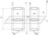 |
Fig. 1 Sketch of the equilibrium configuration (from Robertson & Ruderman 2011). |
2. Derivation of the damping rate
2.1. Equilibrium configuration and governing equations
The system of two coronal loops is modelled as a pair of parallel magnetic cylinders of
length L and radii RL and
RR, as seen in Fig. 1.
The loops consist of a uniform plasma with densities ρL and
ρR with transition layers of width
lL and lR, respectively, in
which the density adjusts itself continuously and monotonically to the value
ρe of the exterior plasma. We adopt the cold plasma
approximation. A constant magnetic field B lies parallel to
the loop axes; we align a Cartesian coordinate system such that the
z-axis points in this direction. We study the problem in bicylindrical
(σ,τ,z) coordinates. A sketch of the bicylindrical coordinate system is
given in Fig. 2. This coordinate system has two
points x = ± a such that all coordinate surfaces
σ = const. pass through these two points. The relation
between Cartesian and bicylindrical coordinates is given by 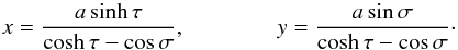 (1)The tube
boundaries can be expressed by τ = − τL and
τ = τR, where
τL,R > 0. The tube radii and the
distance d between the two tube centres can be written in terms of the
parameters of the coordinate system as
(1)The tube
boundaries can be expressed by τ = − τL and
τ = τR, where
τL,R > 0. The tube radii and the
distance d between the two tube centres can be written in terms of the
parameters of the coordinate system as  (2)
(2)
 |
Fig. 2 Sketch of a plane z = const. in the bicylindrical (σ,τ) coordinate system. The lines σ = const. are circles passing through the points x = ± a, the lines τ = const. are nested circles around these points, whose radius tends to zero and whose centre tends to ±a as |τ| → ∞ (from Van Doorsselaere et al. 2008). |
Two geometric limits are relevant throughout the paper. When |τ| → ∞,
the circles τ = const., which are nested around the
points x = ± a, will become smaller and their centres
will converge to the points x = ± a. When
|τ| ≪ 1, the two circles become very large (filling the entire left
and right half-plane in the limit τ → 0). A layer defined by
τ0 < τ < τ0 + l
will become very asymmetric for low values of τ0. The
parameters lL and lR are
essentially parameters of the coordinate system. A physical quantity related to
lL and lR is the mean thickness
of the inhomogeneous layer, defined in bicylindrical coordinates by  (3)The integration in (3) can be carried out and yields
 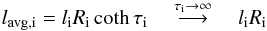 (4)(Robertson & Ruderman 2011), where the subscript
i can be L or R. We impose that the ratios of the average thickness of
the inhomogeneous layers to the tube radii are small parameters,
(4)(Robertson & Ruderman 2011), where the subscript
i can be L or R. We impose that the ratios of the average thickness of
the inhomogeneous layers to the tube radii are small parameters,
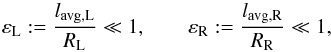 (5)in order to
conserve the ring-like shape of the inhomogeneous layers. This is the thin boundary (TB)
assumption. The TB assumption breaks down when τL,R is not
large enough.
(5)in order to
conserve the ring-like shape of the inhomogeneous layers. This is the thin boundary (TB)
assumption. The TB assumption breaks down when τL,R is not
large enough.
Averaging over the different directions has consequences for the damping properties of the two-loop system, especially for small loop distances. We address them in Sect. 3.1.
Following Ruderman & Roberts (2002) and
Robertson & Ruderman (2011) we have used
the linearised viscous MHD equations to describe the plasma motions. They are given by
![Mathematical equation: \begin{eqnarray} \label{basisvgl} \rho \frac{\partial^2 \boldsymbol{\xi}}{\partial t^2} &=& \frac{1}{\mu_0} \, (\nabla \times \boldsymbol{b}) \times \boldsymbol{B} + \frac{\partial}{\partial t} [\nabla (\overline{\nu} \, \nabla \cdot \boldsymbol{\xi}) - \nabla \times (\overline{\nu} \, \nabla \times \boldsymbol{\xi}) ], \\ \label{basismagnH4}\boldsymbol{b} &=& \nabla \times ( \boldsymbol{\xi} \times \boldsymbol{B}) . \end{eqnarray}](/articles/aa/full_html/2014/02/aa22755-13/aa22755-13-eq38.png) Here
Here
 denotes the
coefficient of shear viscosity, ξ is the Lagrangian
displacement vector, μ0 the permeability of free space, and
b denotes the perturbation of the magnetic field.
Viscosity is important only in a narrow dissipative layer about the Alfvén resonant
surface. This is the magnetic surface where the equation
Re ω = ωA is satisfied, where
ωA is the Alfvén frequency defined by
denotes the
coefficient of shear viscosity, ξ is the Lagrangian
displacement vector, μ0 the permeability of free space, and
b denotes the perturbation of the magnetic field.
Viscosity is important only in a narrow dissipative layer about the Alfvén resonant
surface. This is the magnetic surface where the equation
Re ω = ωA is satisfied, where
ωA is the Alfvén frequency defined by
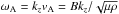 ,
vA is the Alfvén speed, and
kz the parallel wavenumber. In previous
studies that used cylindrical coordinates, the damping rate has been found to be
independent of when this
parameter is small (e.g. Poedts & Kerner
1991; Goossens et al. 1992; Ruderman & Roberts 2002) because of the ideal
nature of the damping mechanism. We can assume a priori that this is also the case in the
two-loop system. Hence it does not matter whether we use the viscous or resistive MHD
equations to describe resonant damping. The eigenfunctions and location of heating are
dependent on the dissipative mechanism (Van Doorsselaere
et al. 2007), but we are not concerned with these problems in this paper.
,
vA is the Alfvén speed, and
kz the parallel wavenumber. In previous
studies that used cylindrical coordinates, the damping rate has been found to be
independent of when this
parameter is small (e.g. Poedts & Kerner
1991; Goossens et al. 1992; Ruderman & Roberts 2002) because of the ideal
nature of the damping mechanism. We can assume a priori that this is also the case in the
two-loop system. Hence it does not matter whether we use the viscous or resistive MHD
equations to describe resonant damping. The eigenfunctions and location of heating are
dependent on the dissipative mechanism (Van Doorsselaere
et al. 2007), but we are not concerned with these problems in this paper.
Finally, to obtain analytical progress, we assume that the loop length L
is much larger than the size of the system in the transverse direction d
(the long-wavelength approximation):
 (8)Here we will study the
eigenvalue problem. The boundary condition at the ends of the loops is the frozen-in
condition at the photosphere at
z = ± L/2, that is
(8)Here we will study the
eigenvalue problem. The boundary condition at the ends of the loops is the frozen-in
condition at the photosphere at
z = ± L/2, that is 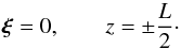 (9)This quantises the
axial wavenumber kz as
(9)This quantises the
axial wavenumber kz as
 . The
boundary conditions across the layers is given in the next subsection.
. The
boundary conditions across the layers is given in the next subsection.
2.2. Boundary conditions across the dissipative layer
We are not interested in the behaviour of the solutions in the dissipative layer itself. By solving the linearised MHD equations separately in the core and outer region and in the dissipative layer, we can match the local solutions to obtain boundary conditions across the dissipative layer in the form of jump conditions. This approach has often been used in the study of resonant absorption in cylindrical geometry, for example by Sakurai et al. (1991), and Goossens et al. (1995) for the driven problem and Tirry & Goossens (1996) for the eigenvalue problem, and has recently been adapted to a bicylindrical coordinate system by Robertson & Ruderman (2011). Hence we limit ourselves in this subsection to citing the major results needed in the remainder of the paper.
Van Doorsselaere et al. (2008) have computed the
eigenmodes of the two-loop system analytically in the long-wavelength limit if we replace
the inhomogeneous layers by discontinuous jumps in density from
ρL,R to ρe. We introduce the
dispersion function ![Mathematical equation: \begin{eqnarray} \label{definitionD0} D_0 (\omega) := F^2 \omega^4 (\rho_{\textrm{L}} - \rho_\textrm{e}) (\rho_{\textrm{R}} - \rho_\textrm{e}) &&- \left[(\rho_{\textrm{L}} + \rho_\textrm{e}) \omega^2- 2\rho_\textrm{e} v_\textrm{Ae}^2 k^2\right] \nonumber \\ &&\hspace*{-4mm}\times \left[(\rho_{\textrm{R}} + \rho_\textrm{e}) \omega^2 - 2 \rho_\textrm{e} v_\textrm{Ae}^2 k^2\right] \end{eqnarray}](/articles/aa/full_html/2014/02/aa22755-13/aa22755-13-eq53.png) (10)to
write the dispersion relation of Van Doorsselaere et al.
(2008) as
(10)to
write the dispersion relation of Van Doorsselaere et al.
(2008) as  (11)with solutions
 (12)In these equations
ζL,R = ρL,R/ρe
are the normalised densities and
F = exp [−(τL + τR)]
is a geometric factor.
(12)In these equations
ζL,R = ρL,R/ρe
are the normalised densities and
F = exp [−(τL + τR)]
is a geometric factor.
The normal modes of the homogeneous two-loop system have previously been studied numerically by Luna et al. (2008). They found four eigenfrequencies that can be split into two pairs of frequencies that lie very close to one another, instead of the two eigenfrequencies described by Eq. (12). The four different eigenmodes can be classified as symmetric (S) or antisymmetric (A), and the displacement can be either in the x- or the y-direction. The lowest frequencies are found for the Sx and Ay eigenmodes. The long-wavelength assumption ignores the dispersion between the two eigenmode pairs and reduces the number of normal modes of the system from four to two.
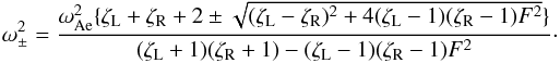
Note that ω+ is a monotonically decreasing function of
τL + τR and
ω− is a monotonically increasing function of
τL + τR, with limits
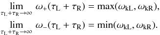 (13)Here
ωki is the kink frequency defined by
(13)Here
ωki is the kink frequency defined by 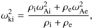 (14)where again the subscript
i can be either L or R. Equation (13)
shows that for large loop separations, the system of coronal loops becomes decoupled. The
collective eigenfrequencies tend to the kink eigenfequencies of the individual loops. A
consequence of the limits (13) is that for
two nonidentical loops (by convention, we set
ζL < ζR
in this case) a region in the plane determined by
ζL/ζR and
τL + τR (i.e. density contrast
and distance between the loops) always exists such that
ω− < ωAL
(Van Doorsselaere et al. 2008). Systems of two
coronal loops in which this situation occurs are called anomalous.
(14)where again the subscript
i can be either L or R. Equation (13)
shows that for large loop separations, the system of coronal loops becomes decoupled. The
collective eigenfrequencies tend to the kink eigenfequencies of the individual loops. A
consequence of the limits (13) is that for
two nonidentical loops (by convention, we set
ζL < ζR
in this case) a region in the plane determined by
ζL/ζR and
τL + τR (i.e. density contrast
and distance between the loops) always exists such that
ω− < ωAL
(Van Doorsselaere et al. 2008). Systems of two
coronal loops in which this situation occurs are called anomalous.
The introduction of a thin inhomogeneous layer leads to a continuous Alfvén spectrum. At the Alfvén resonant magnetic surface, defined by Re ω = ωA, the ideal MHD equations become “quasi-singular” (Soler et al. 2013). For the two-loop system, we calculated that just as in cylindrical geometry, the eigenfrequencies are complex and hence the resonant position does not lie on the real axis in the complex plane. This means there are no actual singularities in the ideal MHD equations. In resistive MHD, the quasi-singularities are lifted and the quasi-modes found in ideal MHD become proper resistive eigenmodes.
When a smooth initial perturbation is applied to the system, each surface resonates at its own Alfvén frequency. Energy pumped into the inhomogeneous layer is converted into local Alvén wave energy propagating along the magnetic field lines. After a while, the neighbouring magnetic flux surfaces drift out of phase with one another, creating steep gradients on small length scales. These gradients would grow unboundedly in time in ideal MHD, but in resistive MHD the Ohmic dissipation term will dominate locally due to the decrease of the magnetic Reynolds number (phase mixing, see e.g. Heyvaerts & Priest 1983). This converts the wave energy into heat. The global phenomenon of transfer of incident wave energy into energy of local Alfvén waves and its subsequent dissipation on small scales due to finite resistivity is what is meant by resonant absorption (Andries 2003).
The qualitative description of resonant absorption in coronal cylinders (loops, jets, etc.) is independent of the coordinate system and has amassed a substantial literature (starting with Sakurai et al. 1991; Goossens et al. 1995). Improvements on the theory of resonant absorption consist mainly of extensions of the theory to more realistic equilibria and the effects on measurable quantities relevant to coronal seismology such as wave periods and damping times.
Recently, the applicability of the “classical theory of resonant damping” (M. Ruderman, priv. comm.) to the initial value problem as outlined above has been challenged by Pascoe et al. (2013) and Hood et al. (2013) for propagating kink waves and by Ruderman & Terradas (2013) for standing kink modes. The time (resp. length) scales required to create the large gradients near the resonant layer are of the order of the wave period (wavelength) times Re1/3, where Re is the magnetic Reynolds number. Because Re ≫ 1 in the solar corona, these scales are much larger than the typical damping times (lengths) of the oscillations.
It was found numerically by Pascoe et al. (2013) and analytically by Hood et al. (2013) that the initial spatial damping profile of propagating kink oscillations is better described by a Gaussian damping profile. After a few wavelengths, the exponential damping profile predicted by the classical theory dominates. The same results were found by Ruderman & Terradas (2013) for temporal damping profiles of standing kink waves. These results indicate that the classical theory of resonant absorption underestimates the damping time (length) of the oscillations. The error increases with increasing thickness of the inhomogeneous layer. Ruderman & Terradas (2013) found that for thin boundary layers such as considered here, the error is still lower than 20% for l/R = 0.3. This justifies our use of the classical theory for the two-loop system.
Since ω− lies outside of the Alfvén spectrum of the left loop in anomalous systems, there is only a resonant surface for ω+ in this loop. In all other cases resonant surfaces exist for both eigenfrequencies in both loops.
In the outer and core regions we can use an ideal MHD description. Van Doorsselaere et al. (2008) calculated that the displacement vector
and total pressure perturbation in bicylindrical coordinates there is given by
 (15)
(15) (16)
(16) (17)
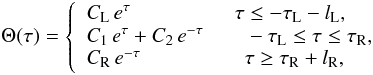
(17)![Mathematical equation: \begin{eqnarray} \label{hatxitauch4} &&\hat{\xi}_{\tau}(\tau) =\left\{ \begin{array}{ll} \dfrac{C_{\textrm{L}} e^{\tau}}{a \rho_{\textrm{L}} (\omega^2 - v_{\textrm{AL}}^2 k^2)} \qquad \tau \leq -\tau_{\textrm{L}} - l_{\textrm{L}}, \\[4mm] \dfrac{C_1 e^{\tau} - C_2 e^{-\tau}}{a \rho_\textrm{e} (\omega^2 - v_{\textrm{Ae}}^2 k^2)} \qquad -\tau_{\textrm{L}} \leq \tau \leq \tau_{\textrm{R}}, \\[4mm] \dfrac{-C_{\textrm{R}} e^{-\tau}}{a \rho_{\textrm{R}} (\omega^2 - v_{\textrm{AR}}^2 k^2)} \qquad \tau \geq \tau_{\textrm{R}} + l_\textrm{R}, \end{array} \right. \end{eqnarray}](/articles/aa/full_html/2014/02/aa22755-13/aa22755-13-eq80.png) (18)in
which
CL,C1,C2
and CR are constants to be determined by the boundary
conditions across the inhomogeneous layers.
(18)in
which
CL,C1,C2
and CR are constants to be determined by the boundary
conditions across the inhomogeneous layers.
In the dissipative layer we use the viscous MHD equations. Robertson & Ruderman (2011) found that, just as in cylindrical
coordinates, the τ-dependence of the total pressure Θ can be taken
constant,  (19)without further loss
of accuracy. For the τ-component of the displacement vector we have
(19)without further loss
of accuracy. For the τ-component of the displacement vector we have
 (20)where
C is an integration constant and the function
(20)where
C is an integration constant and the function  (21)also appears in studies
of eigenmodes of dissipative MHD in Cartesian (Ruderman et
al. 1995) and cylindrical (Tirry &
Goossens 1996) geometry. These functions depend on the density
ρA and the gradient of Alfvén frequency squared | Δ | at the
resonant surface. In the eigenvalue problem the former only depends on the real part of
the eigenfrequency of the two-loop system by definition of the resonant surface. Here
ρA and | Δ | are given by
(21)also appears in studies
of eigenmodes of dissipative MHD in Cartesian (Ruderman et
al. 1995) and cylindrical (Tirry &
Goossens 1996) geometry. These functions depend on the density
ρA and the gradient of Alfvén frequency squared | Δ | at the
resonant surface. In the eigenvalue problem the former only depends on the real part of
the eigenfrequency of the two-loop system by definition of the resonant surface. Here
ρA and | Δ | are given by  The
jump of any quantity f across the dissipative layer is defined as
The
jump of any quantity f across the dissipative layer is defined as
![Mathematical equation: \begin{equation} \label{jumpch4} [f] = \lim_{h \rightarrow 0} \, \{f(\tau_\textrm{i} + h) - f(\tau_\textrm{i} - h)\}. \end{equation}](/articles/aa/full_html/2014/02/aa22755-13/aa22755-13-eq93.png) (24)Asymptotic
matching of the local ideal and viscous equations leads to the following jump conditions
across the dissipative layer: for standard systems
(24)Asymptotic
matching of the local ideal and viscous equations leads to the following jump conditions
across the dissipative layer: for standard systems ![Mathematical equation: \begin{eqnarray} \label{thetajumpch4} [\Theta] &=& 0, \\ \label{jumpxitauch4} [\hat{\xi}_{\tau}] &=& - \frac{i \pi \Theta(\tau_{\rm A})}{a \rho_{\textrm{A}} |\Delta|} \end{eqnarray}](/articles/aa/full_html/2014/02/aa22755-13/aa22755-13-eq94.png) holds
for both loops. In anomalous systems the absence of a resonant surface for the lower
eigenfrequency in the left loop means that only one resonant surface in the left loop
remains, defined by ω+ = ωAL. We
can use the same formulae for standard and anomalous systems if we redefine the jump
condition (26) for anomalous systems as
follows:
holds
for both loops. In anomalous systems the absence of a resonant surface for the lower
eigenfrequency in the left loop means that only one resonant surface in the left loop
remains, defined by ω+ = ωAL. We
can use the same formulae for standard and anomalous systems if we redefine the jump
condition (26) for anomalous systems as
follows: ![Mathematical equation: \begin{equation} \label{jumpxitauanomalousch4} [\hat{\xi}_{\tau, \textrm{L,-}}] = 0, \quad [\hat{\xi}_{\tau, \textrm{L,+}}] = - \frac{i \pi \Theta(\tau_{\textrm{AL}})}{a \rho_{\textrm{A}} |\Delta_{\textrm{L}}|}, \; [\hat{\xi}_{\tau, \textrm{R}}] = - \frac{i \pi \Theta(\tau_{\textrm{AR}})}{a \rho_{\textrm{A}} |\Delta_{\textrm{R}}|}\cdot \end{equation}](/articles/aa/full_html/2014/02/aa22755-13/aa22755-13-eq96.png) (27)
(27)
2.3. Dispersion relation and damping rate
We use the jump conditions (25), (26), and (27) to derive an expression for the damping rate γ for two loops with arbitrary densities. One approach is to integrate these jump conditions across a nonuniform equilibrium to obtain boundary conditions across the entire inhomogeneous layer. This leads to a description in the form of principal value integrals (Robertson & Ruderman 2011).
Another, simpler, approach can be motivated as follows: the dissipative solutions (19) and (20) are local in the sense that they were obtained using a Taylor expansion of the Alfvén frequency at the resonant layer. If we assume that the density profile is almost linear in the inhomogeneous layer, Eqs. (19) and (20) can be considered valid across the entire inhomogeneous layer. Then the jump conditions (25), (26), and (27) can be used across this layer as well.
We do not lose any generality compared to almost all previous studies using the TB
assumption, which assumed linear or sinusoidal density profiles in the nonuniform layer.
Furthermore, in cylindrical coordinates, the only effect of the density profile is a
constant factor appearing in solutions for the damping rate (see Eq. (77) of Goossens et al. 2002, which needs to be corrected for a
typo: the factor  needs to be squared). This
expression only depends in fact on the gradient of the Alfvén speed at the resonance
through the factor 1/Δ. One needs determine a posteriori whether this
dependence still holds in bicylindrical coordinates. It is important to note that the
density profile does matter when we consider thick inhomogeneous layers (Soler et al. 2013).
needs to be squared). This
expression only depends in fact on the gradient of the Alfvén speed at the resonance
through the factor 1/Δ. One needs determine a posteriori whether this
dependence still holds in bicylindrical coordinates. It is important to note that the
density profile does matter when we consider thick inhomogeneous layers (Soler et al. 2013).
A second argument in favour of our approach is that ultimately, retention of the principal value integrals in the calculations only leads to a phase shift of the eigenfunctions and does not influence the imaginary part γ of the eigenfrequency (Robertson & Ruderman 2011). By dropping the principal value integral from the start, we can calculate more general expressions for the damping rate than were found by Robertson & Ruderman (2011).
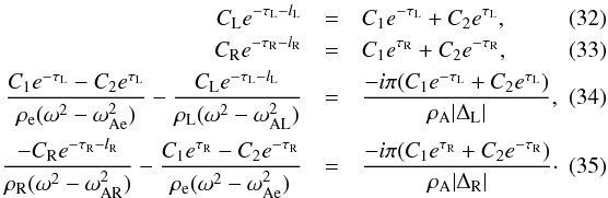
We focus on the case of standard systems. The derivation for standard and anomalous
systems is similar; the results for anomalous systems are given at the end of the
derivation. The jump conditions across the inhomogeneous layer are ![Mathematical equation: \begin{eqnarray} \label{BC_inhomogeneous1}\hat{\xi}_{\tau}(-\tau_{\textrm{L}}) - \hat{\xi}_{\tau}(-\tau_{\textrm{L}} - l_{\textrm{L}}) = [\hat{\xi}_{\tau, \textrm{L}}] &=& - \frac{i \pi \Theta(\tau_{\textrm{AL}})}{a \rho_{\textrm{A}} |\Delta_{\textrm{L}}|}, \\ \label{BC_inhomogeneous2} \Theta(-\tau_{\textrm{L}} - l_{\textrm{L}}) - \Theta(-\tau_{\textrm{L}}) &=& 0, \\ \label{BC_inhomogeneous3} \hat{\xi}_{\tau}(\tau_{\textrm{R}} + l_\textrm{R}) - \hat{\xi}_{\tau}(\tau_{\textrm{R}}) = [\hat{\xi}_{\tau, \textrm{R}}] &=& - \frac{i \pi \Theta(\tau_{\textrm{AR}})}{a \rho_{\textrm{A}} |\Delta_{\textrm{R}}|}, \\ \label{BC_inhomogeneous4} \Theta(\tau_{\textrm{R}} + l_\textrm{R}) - \Theta(\tau_{\textrm{R}}) &=& 0. \end{eqnarray}](/articles/aa/full_html/2014/02/aa22755-13/aa22755-13-eq100.png) Equations
(28)–(31) are the appropriate boundary conditions to be used in Eqs. (16) and (18). Since Θ is constant across the annuli, we can take
ΘAL = Θ(−τL − lL) = C1e− τL + C2eτL
in the left annulus and
ΘAR = Θ(τR + lR) = C1eτR + C2e− τR
in the right annulus. This yields the following system of equations:
Equations
(28)–(31) are the appropriate boundary conditions to be used in Eqs. (16) and (18). Since Θ is constant across the annuli, we can take
ΘAL = Θ(−τL − lL) = C1e− τL + C2eτL
in the left annulus and
ΘAR = Θ(τR + lR) = C1eτR + C2e− τR
in the right annulus. This yields the following system of equations:
 This
system has a nontrivial solution for
C1,...,C4
only if its coefficient matrix has a determinant equal to zero. We now introduce the
notation
This
system has a nontrivial solution for
C1,...,C4
only if its coefficient matrix has a determinant equal to zero. We now introduce the
notation 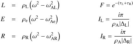 (36)to
write the dispersion relation for ω2 as
(36)to
write the dispersion relation for ω2 as ![Mathematical equation: \begin{eqnarray} \label{dispersiestief} D_0(\omega) &=& -E R I_\textrm{R} [F^2(L-E)+(L+E)] \nonumber \\ &&\quad - E L I_\textrm{L} [F^2 (R-E) + (R+E)] + E^2 L R I_\textrm{L} I_\textrm{R} \left(1-F^2\right), \end{eqnarray}](/articles/aa/full_html/2014/02/aa22755-13/aa22755-13-eq107.png) (37)where
D0(ω) was introduced in (10). By Eqs. (36), the final term on the right-hand side of (37) is proportional to
1/|ΔL|·1/|ΔR |. For
quasi-linear density profiles, we see in Eq. (52) that this term is proportional to
εL·εR and hence can be ignored
with respect to the other terms, which are of the order of
εL,R. We can then isolate the terms
εL,R in the right-hand side of Eq. (37) and write the right-hand side compactly as
εDε(ω).
This yields the dispersion relation
(37)where
D0(ω) was introduced in (10). By Eqs. (36), the final term on the right-hand side of (37) is proportional to
1/|ΔL|·1/|ΔR |. For
quasi-linear density profiles, we see in Eq. (52) that this term is proportional to
εL·εR and hence can be ignored
with respect to the other terms, which are of the order of
εL,R. We can then isolate the terms
εL,R in the right-hand side of Eq. (37) and write the right-hand side compactly as
εDε(ω).
This yields the dispersion relation  (38)where
 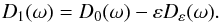 (39)Since the introduction
of a thin inhomogeneous layer only represents a weak perturbation to the system, it is
logical to search for solutions in the neighbourhood of ω±.
Hence we develop D1(ω) in a Taylor series
about ω = ω±:
(39)Since the introduction
of a thin inhomogeneous layer only represents a weak perturbation to the system, it is
logical to search for solutions in the neighbourhood of ω±.
Hence we develop D1(ω) in a Taylor series
about ω = ω±: ![Mathematical equation: \begin{eqnarray} \label{Taylordispersion} D_1(\omega) \approx D_1(\omega_\pm + \varepsilon \delta\omega) &=& D_0(\omega_\pm) + \varepsilon D_\varepsilon(\omega_\pm) \nonumber \\ &&\quad + \varepsilon \, \delta \omega \left[ \frac{\partial D_0(\omega)}{\partial \omega} \right]_{\omega = \omega_\pm} + O\left(\varepsilon^2\right). \end{eqnarray}](/articles/aa/full_html/2014/02/aa22755-13/aa22755-13-eq118.png) (40)Using
Eqs. (11) and (12) for the frequencies of the dissipationless
system in Eq. (40) yields
(40)Using
Eqs. (11) and (12) for the frequencies of the dissipationless
system in Eq. (40) yields
![Mathematical equation: \begin{equation} \delta \omega = \frac{D_\varepsilon(\omega)}{[ \partial D_0(\omega) / \partial \omega ]_{\omega = \omega_\pm}}\cdot \end{equation}](/articles/aa/full_html/2014/02/aa22755-13/aa22755-13-eq119.png) (41)Equations (36) and (37) imply that
Dε(ω) is purely imaginary.
This means that δω is also imaginary, hence we write
δω = iγ, where γ is the damping rate
we aim to determine. In conclusion, introducing a thin inhomogeneous layer only introduces
damping of the eigenmodes and does not result in a frequency shift of the oscillations.
(41)Equations (36) and (37) imply that
Dε(ω) is purely imaginary.
This means that δω is also imaginary, hence we write
δω = iγ, where γ is the damping rate
we aim to determine. In conclusion, introducing a thin inhomogeneous layer only introduces
damping of the eigenmodes and does not result in a frequency shift of the oscillations.
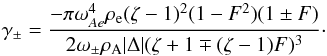
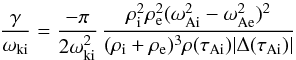
After some algebra, we obtain the following expression of the damping rate for the
transverse oscillations in a system of two parallel coronal loops: ![Mathematical equation: \begin{eqnarray} \label{dampingch4twotubes} \dfrac{\gamma_{\pm}}{\omega_\pm} &=& \dfrac{- \pi (\omega_\pm^2 - \omega_{\text{Ae}}^2)}{\mp 4 \omega_\pm^2 \rho_\textrm{e} \omega_{\text{Ae}}^2 \rho_{\textrm{A}} \sqrt{(\zeta_{\textrm{L}} - \zeta_{\textrm{R}})^2 + 4 (\zeta_{\textrm{L}} - 1)(\zeta_{\textrm{R}} - 1) F^2}} \nonumber \\ && \, \nonumber \\ && \hspace*{-4mm}\times \Bigg( \dfrac{\rho_{\textrm{R}} (\omega_\pm^2 - \omega_{\text{AR}}^2) [(1+F^2) \rho_{\textrm{L}} (\omega_\pm^2 - \omega_{\text{AL}}^2) + (1-F^2) \rho_\textrm{e} (\omega_\pm^2 - \omega_{\text{Ae}}^2)]}{|\Delta_{\textrm{R}}|} \nonumber \\ && \, \nonumber \\ &&\hspace*{-4mm} + \dfrac{\rho_{\textrm{L}} (\omega_\pm^2 - \omega_{\text{AL}}^2) [(1+F^2) \rho_{\textrm{R}} (\omega_\pm^2 - \omega_{\text{AR}}^2) + (1-F^2) \rho_\textrm{e} (\omega_\pm^2 - \omega_{\text{Ae}}^2)]}{|\Delta_{\textrm{L}}|}\Bigg)\cdot \end{eqnarray}](/articles/aa/full_html/2014/02/aa22755-13/aa22755-13-eq123.png) (42)The
two last terms describe the contribution of the resonances in both loops (through the
factors 1/|ΔL,R |) to the total damping rate. The meaning
of these terms is discussed in detail in Sect. 3. Formally, the equations for the damping
rate in the left loop in an anomalous system can be obtained from the equations of a
standard system by letting | ΔL| → ∞. For future reference, we will write
down the equation for the damping rate in anomalous systems, which is
(42)The
two last terms describe the contribution of the resonances in both loops (through the
factors 1/|ΔL,R |) to the total damping rate. The meaning
of these terms is discussed in detail in Sect. 3. Formally, the equations for the damping
rate in the left loop in an anomalous system can be obtained from the equations of a
standard system by letting | ΔL| → ∞. For future reference, we will write
down the equation for the damping rate in anomalous systems, which is ![Mathematical equation: \begin{eqnarray} \label{dampingch4twotubesanom} \dfrac{\gamma_{-,\text{a}}}{\omega_-} &=& \dfrac{- \pi (\omega_\pm^2 - \omega_{\text{Ae}}^2)}{\mp 4 \omega_\pm^2 \rho_\textrm{e} \omega_{\text{Ae}}^2 \rho_{\textrm{A}} \sqrt{(\zeta_{\textrm{L}} - \zeta_{\textrm{R}})^2 + 4 (\zeta_{\textrm{L}} - 1)(\zeta_{\textrm{R}} - 1) F^2}} \nonumber \\ && \, \nonumber \\ &&\times \dfrac{\rho_{\textrm{R}} (\omega_\pm^2 - \omega_{\text{AR}}^2) [(1+F^2)\rho_{\textrm{L}} (\omega_\pm^2 - \omega_{\text{AL}}^2) + (1-F^2) \rho_\textrm{e} (\omega_\pm^2 - \omega_{\text{Ae}}^2)]}{|\Delta_{\textrm{R}}|}\cdot \end{eqnarray}](/articles/aa/full_html/2014/02/aa22755-13/aa22755-13-eq126.png) (43)Expression
(42) generalises several results found
previously in studies of two-loop oscillations. Firstly, if we remove dissipation, this
means we set
IL = 0,IR = 0
in Eq. (37), then substituting the
relations (36) in this reduced dispersion
relation leads back to Eq. (11) found by
Van Doorsselaere et al. (2008).
(43)Expression
(42) generalises several results found
previously in studies of two-loop oscillations. Firstly, if we remove dissipation, this
means we set
IL = 0,IR = 0
in Eq. (37), then substituting the
relations (36) in this reduced dispersion
relation leads back to Eq. (11) found by
Van Doorsselaere et al. (2008).
Secondly, we consider what happens when the tubes are identical. Such systems exhibit the
standard behavior independent of the separation between the loops. The two terms in the
second factor of (42) are then also
identical. After some algebra, we find that the expression for the damping rate becomes
 (44)This equation is
identical to Eq. (82) of Robertson & Ruderman
(2011), up to a sign, since these authors write
ω ≈ ω± − iγ, while we used
ω ≈ ω± + iγ.
(44)This equation is
identical to Eq. (82) of Robertson & Ruderman
(2011), up to a sign, since these authors write
ω ≈ ω± − iγ, while we used
ω ≈ ω± + iγ.
Finally, we consider the case d/R → ∞ in which the tubes are placed far away from each other. This situation corresponds mathematically to τL + τR → ∞ or F → 0. Even though the loop centres converge to x = ± a and hence remain at a finite distance from one another, compared to their radius (which is the typical length scale of the loops), the loops will diverge infinitely far apart from each other.
We note that in the long-wavelength approximation and using bicylindrical coordinates, it
is in fact impossible to realise a configuration of loops that are far apart without
shrinking to a zero thickness. This is because the Eqs. (2) imply  (45)while the
long-wavelength assumption together with (2) implies that
(45)while the
long-wavelength assumption together with (2) implies that 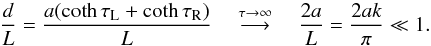 (46)Equation (46) demands that ak ≪ 1 such
that from Eq. (45) it follows that
RL,R/LL,R → 0
as τL + τR → ∞.
(46)Equation (46) demands that ak ≪ 1 such
that from Eq. (45) it follows that
RL,R/LL,R → 0
as τL + τR → ∞.
When the loops are placed far away from one another, we expect that the loops oscillate
independently from one another. Indeed, using the limits (13) on Eq. (42) (in
this limiting case, the system always exhibits the standard behaviour) and substituting
ωki in the resulting expression by (14), we recover after some algebra the formula
 (47)for
the damping rate. This result is valid for both loops. We compared this equation to Eq.
(77) of Goossens et al. (1992). Since the
thicknesses of the inhomogeneous layers can vary with position (see the remarks concerning
Fig. 2), we compared Eq. (47) with the
damping rates of equivalent tubes described in cylindrical geometry whose inhomogeneous
layers are rings whose thickness equals the average thickness of the original layers,
described in bicylindrical coordinates. If we assume that the density in the inhomogeneous
layer varies almost linearly from its value in the core to the value of the outside
plasma, then Eq. (4) implies for the loops
described in bicylindrical coordinates that
(47)for
the damping rate. This result is valid for both loops. We compared this equation to Eq.
(77) of Goossens et al. (1992). Since the
thicknesses of the inhomogeneous layers can vary with position (see the remarks concerning
Fig. 2), we compared Eq. (47) with the
damping rates of equivalent tubes described in cylindrical geometry whose inhomogeneous
layers are rings whose thickness equals the average thickness of the original layers,
described in bicylindrical coordinates. If we assume that the density in the inhomogeneous
layer varies almost linearly from its value in the core to the value of the outside
plasma, then Eq. (4) implies for the loops
described in bicylindrical coordinates that 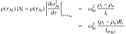 (48)This
is equal to Ri times the corresponding value of
ρAi |Δ | for the equivalent loops in cylindrical
coordinates. Substituting Eq. (48) into
(47) exactly gives Eq. (77) of Goossens et al. (1992). This perfect agreement between
the two coordinate systems is possible only because the geometric term
cothτi vanishes in Eq. (4) in the limit τi → ∞. For loops closer to
one another, geometric effects due to the variation of annulus thickness will play a role.
(48)This
is equal to Ri times the corresponding value of
ρAi |Δ | for the equivalent loops in cylindrical
coordinates. Substituting Eq. (48) into
(47) exactly gives Eq. (77) of Goossens et al. (1992). This perfect agreement between
the two coordinate systems is possible only because the geometric term
cothτi vanishes in Eq. (4) in the limit τi → ∞. For loops closer to
one another, geometric effects due to the variation of annulus thickness will play a role.
3. Parametric study of the damping rate
In this section we study the dependence of the damping rate γ, given in
Eqs. (42) and (43), on the separation distance
d/R between the loops and the density
contrast between the two loops. We assume that both loops have the same radius, since the
numerical calculations of Luna et al. (2008) of
eigenoscillations of a two-loop system – without restriction to long wavelengths – showed
that the eigenfrequencies only weakly depend on the tube radius. For analytical simplicity
we suppose that the density profile is linear throughout the inhomogeneous layers
τ ∈ { −τi − l, − τi }
and
τ ∈ { τi,τi + l }:
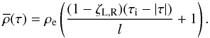 (49)Here
τi = τL = τR
and the subscripts L and R are dropped for clarity of notation where possible. In Eq. (49) the relative density
ζL was used for τ < 0
and ζR was used for
τ > 0. With this density profile we have
(49)Here
τi = τL = τR
and the subscripts L and R are dropped for clarity of notation where possible. In Eq. (49) the relative density
ζL was used for τ < 0
and ζR was used for
τ > 0. With this density profile we have
 (50)We need the thin boundary
assumption to be valid throughout the entire parameter space. We know, however, that the
tube radius and the shape of the inhomogeneous layer strongly depend on the value of
τi. The most straightforward solution is to fix the average
relative thickness of the nonuniform layer
lavg/R (defined in (3)) to a small number. This also ensures that the
expressions for the damping rate become independent of the radius. Finally, all length
scales were normalised with respect to the loop length L and the density
was normalised with respect to the density ρe of the exterior
plasma, that is,
ζ = ρ/ρe.
As a consequence, all frequencies are normalised with respect to the Alfvén speed of the
exterior medium,
ω → ω/ωAe.
(50)We need the thin boundary
assumption to be valid throughout the entire parameter space. We know, however, that the
tube radius and the shape of the inhomogeneous layer strongly depend on the value of
τi. The most straightforward solution is to fix the average
relative thickness of the nonuniform layer
lavg/R (defined in (3)) to a small number. This also ensures that the
expressions for the damping rate become independent of the radius. Finally, all length
scales were normalised with respect to the loop length L and the density
was normalised with respect to the density ρe of the exterior
plasma, that is,
ζ = ρ/ρe.
As a consequence, all frequencies are normalised with respect to the Alfvén speed of the
exterior medium,
ω → ω/ωAe.
3.1. Dependence on the separation between loops
 |
Fig. 3 Plot of the lower eigenfrequency ω− (full line) as a function of tube separation d/R, together with the Alfvén frequency of the left tube (dotted line), marking the transition point between standard and anomalous systems, and the kink frequency of the right tube (dashed line). |
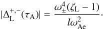
First we investigated the dependence of the damping rate on the separation distance between the two loops. From (2) we know that d/R = 2coshτi. We investigated two cases. In the first case, the loop densities are equal: ζL = ζR = 3. This means we can use the standard expression (42) for the damping rate everywhere. In the second case, we set ζL = 2.5, ζR = 2.9. As Fig. 3 shows, only for very small distances (d/R ≲ 2.05) do we need to use the anomalous expression (43) to determine γ−. It can be read off from Eqs. (42) and (43) that in the limit ω− → ωAL the damping rates of the transverse oscillations in standard and anomalous systems converge to the same value, such that γ− is a continuous function of both density and distance at this frequency.
 |
Fig. 4 Dependence of the damping rate γ/ω0 (where ω0 can be either ω+ or ω−) on the separation between the loops. a) Equal loop densities ζL = ζR = 3. b) Unequal loop densities ζL = 2.5, ζR = 2.9. The damping rate corresponding to ω− is shown as full lines, while the damping rate corresponding to ω+ is shown as thick dashed lines. The damping rates for the kink oscillations of the individual loops (thin dashed and dotted lines) are also shown. |
Figure 4 shows how the damping properties of the
two-loop system vary with increasing distance between the loops. The damping of the kink
frequencies of the individual flux tubes are given by 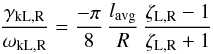 (51)(Goossens et al. 1992). For both eigenfrequencies the
sign of γ is negative so that we are dealing with an actual damping
mechanism. As is the case in cylindrical coordinates, the results using the TB assumption
predict long damping times in contradiction to observed damping times (Aschwanden et al. 2002).
(51)(Goossens et al. 1992). For both eigenfrequencies the
sign of γ is negative so that we are dealing with an actual damping
mechanism. As is the case in cylindrical coordinates, the results using the TB assumption
predict long damping times in contradiction to observed damping times (Aschwanden et al. 2002).
In the previous subsection, we analytically showed that the damping rates of the two eigenfrequencies converge to the damping rates of the individual loop oscillations because they are placed farther apart.
When the separation between the loops becomes smaller, they interact more strongly
because the collective homogeneous eigenfrequencies differ more from the individual kink
frequencies, as can be seen for the lower eigenfrequency in Fig. 3. Just as in Robertson &
Ruderman (2011), we found that the interaction between the loops reduces the
efficiency of resonant damping. The damping disappears completely in the limit
τi → 0. However, this last fact is due to geometric effects
corresponding to the bicylindrical coordinate system and is not caused by physical
effects. The main effect lies in the factor 1/Δ, which appears in the
expressions (42) and (43) of the damping rate. Equations (4) and (50) can be combined to yield  (52)The quantity
l is linked to the coordinate system, while we fixed the physical
quantity lavg/R in the
calculations. The limit τi → 0 hence forces
1/|Δ| → 0, even though the inhomogeneous layer does not disappear
here (which is the usual interpretation of this limit). Instead, the inhomogeneous layer
becomes very asymmetric because both loops expand when taking
τi → 0. Hence the limit 1/|Δ| → 0 is
due to geometrical effects, and not because of the disappearance of the resonant damping
mechanism.
(52)The quantity
l is linked to the coordinate system, while we fixed the physical
quantity lavg/R in the
calculations. The limit τi → 0 hence forces
1/|Δ| → 0, even though the inhomogeneous layer does not disappear
here (which is the usual interpretation of this limit). Instead, the inhomogeneous layer
becomes very asymmetric because both loops expand when taking
τi → 0. Hence the limit 1/|Δ| → 0 is
due to geometrical effects, and not because of the disappearance of the resonant damping
mechanism.
Aside from that, one can calculate that the real part of the eigenfrequencies tends to
 (53)as
τi → 0. This causes the term
(53)as
τi → 0. This causes the term
 in Eqs.
(42) and (43) to vanish for the damping rate γ+
corresponding to ω+. The factor (1 ± F) in
Eq. (44) should be identified with
in Eqs.
(42) and (43).
in Eqs.
(42) and (43) to vanish for the damping rate γ+
corresponding to ω+. The factor (1 ± F) in
Eq. (44) should be identified with
in Eqs.
(42) and (43).
When the two loops have equal densities, Eq. (53) yields that  with
with
 the
interior Alfvén frequency of both loops. One can see from the second factor in Eq. (42) that because
(1 − F2) = 0 a factor
the
interior Alfvén frequency of both loops. One can see from the second factor in Eq. (42) that because
(1 − F2) = 0 a factor
 can be factored out,
which vanishes because of (53). These
factors correspond with the term (1 − F2) that appears in
(44). The limits (53) are themselves influenced by the
description in bicylindrical coordinates because of the term
F2 appearing in (12). However, in anomalous systems these terms do not play a role for the lower
frequency as Eq. (43) shows, so the
essence of the problem lies in the terms 1/ΔL,R, as
explained before.
can be factored out,
which vanishes because of (53). These
factors correspond with the term (1 − F2) that appears in
(44). The limits (53) are themselves influenced by the
description in bicylindrical coordinates because of the term
F2 appearing in (12). However, in anomalous systems these terms do not play a role for the lower
frequency as Eq. (43) shows, so the
essence of the problem lies in the terms 1/ΔL,R, as
explained before.
In short, the analysis of the expressions for the damping rate shows that the limit 1/|Δ| → 0 as τi → 0, caused by the geometry of our description, causes the damping rate to go to zero. It follows that the result that the damping rate decreases with decreasing loop distance is also influenced by the geometrical description in bicylindrical coordinates. Indeed, Fig. 9.4 (a) in Soler (2010), who used the T-matrix method, shows that in cylindrical geometry the damping rate of the high-frequency eigenoscillation increases as the loops move closer together. It is not clear how one can separate the geometry from the physics for small loop distances in a description in bicylindrical coordinates.
Because we assumed a linear or quasi-linear density profile, the average thickness of the inhomogeneous layers lavg/R only appears as a constant of proportionality in Eq. (42) (with 1/|Δ | substituted from (52)). The damping rate is proportional to the average thickness of the inhomogeneous layers, as is the case for cylindrical structures in the TB limit. (e.g. Goossens et al. 2009). It is reasonable to assume that the results obtained with the TB assumption can be extrapolated to larger thicknesses of the inhomogeneous layers up to lavg/R ≈ 0.3, as in Van Doorsselaere et al. (2004).
We note from Fig. 4 that the high-frequency oscillations (corresponding to ω+) are more strongly damped than the low-frequency oscillations (corresponding to ω−) for equal loop densities, while for unequal loop densities the faster oscillations are more strongly damped only up to a certain separation distance between the loops. In general, the high-frequency oscillations are more strongly damped when the interaction between the loops is strong. A physical explanation for this can be found when we consider the motions of the intermediate fluid. As Luna et al. (2008) explained, the plasma between the loops moves in such a way that it acts as an additional restoring force for the oscillatory motions of the two-loop system for the eigenmodes corresponding to ω+, while they support the collective motions of the two-loop system for the eigenmodes corresponding to ω−. (In their formulation, there were four eigenfrequencies since they dropped the long-wavelength assumption, but because these frequencies were split into two pairs lying very close to ω±, their argument can be used here as well.) The same holds for the damping rate, which is enhanced by the oppositely directed motions at both sides of the resonant layers for the forced eigenmodes corresponding to ω+. These eigenmodes can be more efficiently damped than the unforced eigenmodes corresponding to ω−. This effect persists until the system decouples at larger separation distances, when the individual kink properties of the loops dominate.
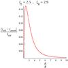 |
Fig. 5 Relative difference between the damping rate of transverse oscillations in standard systems with the equivalent expression for anomalous systems for loop densities ζL = 2.5, ζR = 2.9. (For a given separation distance, only one expression is valid.) |
Finally, Fig. 5 shows the difference between the standard and anomalous expressions (42) and (43) as a function of separation distance. Of the two expressions, only one can be valid for a specified separation distance given the nature of the system as shown in Fig. 3. We see, however, that the relative error one makes by ignoring the standard/anomalous dichotomy is not larger than 15%. The physical reason for this is the following: in anomalous regimes, the less dense loop cannot support the global oscillations of the system anymore (Van Doorsselaere et al. 2008). Hence, the contribution of the damping in this loop to the total damping rate becomes negligible in anomalous systems.
3.2. Dependence on loop densities
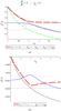 |
Fig. 6 Dependence of the real part ω of the eigenfrequencies and the corresponding damping rate γ/ω in the two-loop system as a function of the density in the right tube ζR for fixed ζL = 3 and d/R = 3. a) Eigenfrequencies ω+ (thick dashed line) and ω− (full line) as a function of ζR, together with the Alfvén frequencies of the left and right tubes (dashed-dotted lines), marking two transition points between standard and anomalous systems (indicated by saR and saL on the horizontal axis, referring to the loop that cannot support the global oscillation), and the individual kink frequencies of the two tubes (dotted and dashed lines). b) Ratio of damping rate to real part of the eigenfrequency of the two-loop system γ/ω0, where ω0 can be either ω+ (thick dashed line) or ω− (full line), and of the left (dotted line) and right (dashed line) loop as a function of ζR. |
In this subsection we investigate the influence of the different tube densities on the damping rate. We set d/R = 3, which is a realistic distance between the loops according to the observations by Aschwanden et al. (2003). We fixed the density of the left loop ζL = 3 and let ζR vary between 1 and 6. This means that either loop can be the less dense one, and that an anomalous system exists at both ends of the density range ζR. This is illustrated in Fig. 6a; the two intersections where such a transition happens are marked on the horizontal axis. A similar dependency of the eigenmodes on the loop densities has been obtained by Luna et al. (2009) using the T-matrix method (see their Fig. 1). For low values of ζR, the right loop cannot support the global oscillations while for high values of ζR, the left loop will be unable to support them. It can be shown that here as well, the contribution of the anomalous regime is negligible because only one loop is oscillating. When the loop densities are equal, the interaction between the loops is maximal since the frequencies ω+ and ω− differ most from the individual kink frequencies.
Figure 6b illustrates the dependence of the observational quantity γ/ω0 (where ω0 can be ω+ or ω−) on the density contrast between the two loops when the distance between them is kept fixed. When the loop densities are equal, the higher eigenfrequency is damped more strongly than for unequal loop densities. The lower eigenfrequency is least damped in this case. Moreover, the damping of the high-frequency oscillation is higher than that of the low-frequency oscillation, |γ+/ω+| > |γ−/ω−|, when the loops have a similar density. The situation is reversed when the relative density contrast between the loops is large.
The reason for this can be found when we analyse Eq. (42) as a function of the two loop densities
ζL and ζR. We isolated the
contribution of each loop to the total damping rate. The only terms that are not invariant
under the permutation ζL ↔ ζR are
the two terms in the second factor of (42). The contribution of these terms is plotted in Fig. 7. We see that the contribution of the term corresponding to the denser
loop dominates the expression for γ−, while the contribution
of the less dense loop dominates in the expression for γ+.
Because the inequality 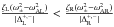 holds when
ζL < ζR
for linear density profiles, this means that the factor
holds when
ζL < ζR
for linear density profiles, this means that the factor
![Mathematical equation: \hbox{$[(1+F^2) \rho_{\textrm{L,R}} (\omega_\pm^2 - \omega_{\text{AL,R}}^2) + (1-F^2) \rho_\textrm{e} (\omega_\pm^2 - \omega_{\text{Ae}}^2)]$}](/articles/aa/full_html/2014/02/aa22755-13/aa22755-13-eq196.png) dominates in the terms describing the contribution from each loop to the total damping
rate.
dominates in the terms describing the contribution from each loop to the total damping
rate.
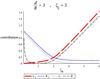 |
Fig. 7 Contribution of the two terms in the last factor of Eq. (42) to the total damping rate of the higher (+) and lower (–) eigenfrequency. The symbols L and R refer to the terms containing 1/|ΔL,R |, respectively. |
The sharper the density contrast, the more substantial the contribution of the denser loop becomes for γ−, and conversely, the more substantial the contribution of the less dense loop becomes for γ+. In these regimes the damping rate γ− can be associated with the damping of the kink oscillation of the denser loop. From this and Eq. (51) for the damping of the individual kink modes by resonant absorption it follows that the low-frequency eigenoscillation is more strongly damped when ζL ≠ ζR.
Soler (2010) noted that even if the real part ω− of the collective oscillation eigenfrequency falls outside of the Alfvén spectrum for one of the loops, the collective eigenmodes can still be efficiently damped due to the resonance in the other loop. This can now be explained for the zero-beta model since the global damping rate γ− depends more on the damping properties of the denser loop. It is reasonable to assume that similar results continue to hold for a finite plasma beta. An interesting question is whether the denser loops also contribute most to the total damping rate of kink-like collective oscillations for systems of more than two coronal loops. This we cannot model using bicylindrical coordinates. We conjecture that the answer in general is affirmative, since Luna et al. (2010) have shown that in a collective oscillation of multiple nonidentical strands, the largest amplitudes occur in the most dense strands for the lowest eigenfrequencies corresponding to kink-like modes and vice versa.
The quantitative results of the previous paragraphs depend on the specific form of the density profile through the gradients of the Alfvén speeds at the resonant surface in the two tubes. About these we do not have much physical information. In particular, if the density profile were different in the two loops, this would affect the relative contribution of both resonances to the global damping of the oscillation. Hence our results are only as accurate as the assumption of quasi-linearity.
When the loop densities are similar,
ζL ≈ ζR, the two terms of the
second factor in (42) become about equally
important because this expression reduces to (44), found by Robertson & Ruderman
(2011), for identical loops. From this equation it is evident that
| γ+/ω+| > |γ−/ω− |.
This is due to two factors: on the one hand (1 ± F), whose spatial
dependence we identified in subsection 3.1. with that of the factor
in Eq. (42). The factor
ζ + 1 ∓ (ζ − 1)F that appears in the
denominator of (44) comes from the
reduction of  when
ζL = ζR. Hence, when the loops
interact more strongly with one another, the difference between
γ+ and γ− is explained
mathematically by the collective oscillation properties of the loops through the factor
ω±. Therefore, we believe that the explanation in terms of
the flow of the intermediate plasma of Luna et al.
(2008), cited when considering the effect of distance between the loops in the
previous subsection, can also physically explain the predicted damping times for the high-
and low-frequency eigenoscillations.
when
ζL = ζR. Hence, when the loops
interact more strongly with one another, the difference between
γ+ and γ− is explained
mathematically by the collective oscillation properties of the loops through the factor
ω±. Therefore, we believe that the explanation in terms of
the flow of the intermediate plasma of Luna et al.
(2008), cited when considering the effect of distance between the loops in the
previous subsection, can also physically explain the predicted damping times for the high-
and low-frequency eigenoscillations.
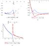 |
Fig. 8 Complex eigenspectrum of the two-loop system and of the left and right loops as a function of ζR. a) Complex spectrum for the higher (crosses) and lower (diagonal crosses) eigenfrequencies of the two-loop system, and the eigenfrequencies of the equivalent left (solid diamond) and right (boxes) loop in cylindrical coordinates as a function of ζR. The damping rates of the left and right loop have been corrected for geometric effects (see text). The parameter ζR increases from 1 to 9 in steps of 0.2. The direction in which the eigenfrequencies move when ζR increases are indicated with arrows. b) Damping rates of the two-loop system γ+ (thick dashed line) and γ− (full line) and of the left (dotted line) and the right (dashed line) loop as a function of ζR. The damping rates of the left and right loop have been corrected for geometric effects (see text). c) The density ζR of the right loop as a function of the eigenfrequencies ω+ (thick dashed line) and ω− (full line) of the two-loop system, and ωkL (dotted line) and ωkR (dashed line) of the left and right loop, respectively. |
When the densities of the two loops approach each other, the eigenoscillation corresponding to ω+ gradually changes its character from being related to the less strongly damped oscillations of the low-density loop to the more heavily damped forced collective oscillations of the two-loop system. The global emerging phenomenon which arises from this is an avoided crossing of the kink modes of the individual loops, as was previously noted by Luna et al. (2009). The characteristics of this phenomenon are now analysed from the same point of view as in the analysis performed by Van Doorsselaere & Poedts (2007) for the complex spectrum of resistive MHD in cylindrical coordinates.
In the complex spectrum shown in Fig. 8a, the complex eigenfrequencies of the two-loop system and of the right loop travel to the left in the complex plane (indicating a decrease in frequency) as ζR increases. The eigenfrequency of the viscous eigenmode of the left loop remains constant since ζL is fixed. The interaction between the loops is the strongest for ζL ≈ ζR with the turning points of the two-loop eigenfrequencies at ζR = 3. A qualitatively similar picture emerges when we fix another value for ζL; the only difference is that the point (ωkL,γkL) moves to the left along the curve defined by (ωkR,γkR) as ζL increases, because expressions (12) and (47) with (48) substituted are the same for both loops.
The effects of avoided crossing on the imaginary part of the eigenfrequencies are illustrated in Fig. 8b. The standard and anomalous expressions (42) and (43) for γ were used where appropriate. In Figs. 8a and 8b the geometrical effects associated with the limits (ζR − 1)/(ζL − 1) → 0 and (ζR − 1)/(ζL − 1) → ∞ calculated when discussing Fig. (6b) were eliminated artificially by multiplying the damping rates of the kink oscillations by tanhτi. The transfer of damping properties of the individual loops from one eigenmode to the other is visible in Fig. 8b, but the convergence of γ+ , − to γkL,R when ζR → ∞ is slower than the convergence of ω+ , − to ωkL,R.
From Fig. 8c we infer that as (ζR − 1)/(ζL − 1) increases, the eigenmode corresponding to ω+ and γ+ transfers some of its properties of the left loop to the eigenmode corresponding to ω− and γ− and inherits the properties of the right loop from it, and vice versa. Near the region where ζL = ζR the collective properties of the two-loop system are dominant.
When the density of the right tube decreases to the density of the exterior fluid, the eigenfrequency ω+ tends to the Alfvén frequency of the exterior fluid (Fig. 6a), since it is the highest frequency present in the system. In this limiting case there remains only one loop, hence γ+ converges to zero in Fig. 6b. The damping rate γ− does not converge to γkL but rather to γkLtanhτi = γkLtanh(arccosh(d/2R)) because of Eqs. (2) and (52). Similarly, we have γ+ → γkLtanhτi and γ− → γkRtanhτi as (ζR − 1)/(ζL − 1) → ∞.
Finally, we compared our results with those of Fig. 9.10 (b) of Soler (2010). The behaviour of damping times as a function of relative loop density for the same equilibrium parameters as considered by Soler (2010) is shown in Fig. 9. The behaviour of the damping times near equal loop densities is the same as we found, and has been explained earlier in this subsection. In Fig. 9.10 (b) of Soler (2010) we have τ−/P− < τ+/P+ for ζR > ζL in the range of values of ζR/ζL shown. This is probably because this range is too narrow, since the limits lim(ζR−1)/(ζL−1)→∞ τ+/P+ = τkL/PkL > τkR/PkR = lim(ζR−1)/(ζL−1)→∞ τ−/P− hold in cylindrical geometry, as is also visible from Fig. 9. Soler (2010) noted that the damping times of the low-frequency eigenoscillations are more weakly dependent on the relative loop densities than the damping times of high-frequency oscillations. This is not the case in our analytic description. The difference can be probably explained by considering that the geometric factors describing the dependence of the damping rate on the separation distance for similar loop densities are slightly different in the description with the T-matrix method than in the description in bicylindrical coordinates.
The results in this section can be compared with those of an equivalent cylindrical loop with a symmetric inhomogeneous layer of width lavg/R (in the sense that geometrical effects do not hide physical effects such as interaction between the loops) when d/R ≳ 4.58 because then tanh(arccoshd/2R) > 0.90. This is a rather large separation distance compared with the observations of Aschwanden et al. (2003). As Fig. 4 of Van Doorsselaere et al. (2008) shows, for such separation distances the loops are already mostly decoupled from one another.
4. Conclusions
We have studied the damped transverse oscillations of a system of two parallel not necessarily identical coronal loops. We restricted ourselves to long wavelengths and thin inhomogeneous layers. For linear or quasi-linear density profiles, we derived analytic expressions for the damping rate γ of the two-loop system that generalise the results found for single cylinders and systems of two identical loops, as we have shown. A subdivision between standard and anomalous systems must be made here.
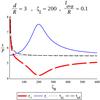 |
Fig. 9 Ratio of damping time to oscillation period of the two-loop system τ/P0, where P0 can be either P+ (thick dashed line) or P− (full line), and of the left (dotted line) and right (dashed line) loop as a function of ζR. The equilibrium parameters have been chosen identical to those of Soler (2010). |
A parametric study to investigate the dependence of γ on the dimensionless parameters led to two important conclusions. Firstly, we saw that the interaction between the loops increases the damping rate of the high-frequency oscillation, while the damping rate of the low-frequency oscillation is reduced by it. The analysis of Eq. (42) showed that for a strong relative density contrast the denser loop contributes most to the damping rate γ− and the less dense loop contributes most to the damping rate γ+, resulting in the inequality |γ+/ω+| < |γ−/ω−| due to the dominating kink-like properties of the loops. On the other hand, for similar loop densities the terms related to ω± dominate the expression for the damping rate. This means that the explanation of Luna et al. (2008) for the different eigenfrequencies of the two-loop system, in terms of the motions of the intermediate fluid, is very likely valid and applicable to the damping rate as well. The intermediate plasma motions act as an additional restoring force for the high-frequency eigenoscillation, which results in shearing motions and an increased damping rate for this collective oscillation, while they support the motions of the low-frequency eigenoscillation, which leads to a decreased damping rate for this collective oscillation. Mathematically, the behaviour of the eigenmodes of the two-loop system as a function of ζR was explained by an avoided crossing of the kink eigenmodes of the individual loops in the complex plane. Our analysis complements the findings of Luna et al. (2008, 2009), Soler (2010) and quantitatively justifies the physical explanation in terms of the motions of the intermediate fluid provided by these authors.
Secondly, we found that in our description, the interaction between the loops reduces the efficiency of resonant damping. However, as conjectured in the final paragraph of Robertson & Ruderman (2011) and confirmed by Eq. (52), this effect is attributed at least partly to the change of shape of the inhomogeneous layer linked to the bicylindrical coordinate system and not to physical effects. Equation (53) shows which terms in the equations for ω± and γ± force the damping rate to vanish in the limit of touching loops.
Even though we also used the bicylindrical coordinate system in this paper, we made clear that there are several problems with this formalism. Summarising, the problems are that
-
1.
it is not possible to preventR → 0 if d/R → ∞.
-
2.
The change of shape of inhomogeneous layer cannot be dealt with in a straightforward way within the bicylindrical coordinate system to investigate the limit of small separation distances between the two loops.
-
3.
The results cannot be generalised to systems of more than two coronal loops.
Therefore we believe additional analytical studies should make use of other mathematical techniques. For a system of two parallel coronal loops, one could look for analytic expressions of the eigenfrequencies and eigenfunctions using the T-matrix method in a local coordinate system, both for undamped and damped oscillations of coronal loops. This would facilitate the comparison with known results from cylindrical geometry. Alternatively, it would be interesting to extend the analysis of Soler (2010) to systems of more than two coronal loops. This approach could lead to a unified understanding of the damped oscillations of systems of coronal loops.
Acknowledgments
The authors thank the referee and Michael Ruderman for valuable comments, which helped improve the content of this paper considerably. S.E.G. acknowledges Arno Kuijlaars and Marcel Goossens for useful discussions. T.V.D. and S.E.G. have received funding from an Odysseus grant of the FWO Vlaanderen and FP7 under grant agreement 276808. We acknowledge the support from Belspo under IAP P7/08 CHARM.
References
- Andries, J. 2003, Ph.D. thesis, KU Leuven [Google Scholar]
- Andries, J., Arregui, I., & Goossens, M. 2005, ApJ, 624, L57 [NASA ADS] [CrossRef] [Google Scholar]
- Arregui, I., & Asensio Ramos, A. 2011, ApJ, 740, 44 [NASA ADS] [CrossRef] [Google Scholar]
- Arregui, I., Andries, J., Van Doorsselaere, T., Goossens, M., & Poedts, S. 2007, A&A, 463, 333 [NASA ADS] [CrossRef] [EDP Sciences] [Google Scholar]
- Arregui, I., Terradas, J., Oliver, R., & Luis Ballester, J. 2008, ApJ, 674, 1179 [NASA ADS] [CrossRef] [Google Scholar]
- Arregui, I., Asensio Ramos, A., & Díaz, A. J. 2013, ApJ, 765, L23 [NASA ADS] [CrossRef] [Google Scholar]
- Aschwanden, M. J., & Schrijver, C. J. 2011, ApJ, 736, 102 [NASA ADS] [CrossRef] [Google Scholar]
- Aschwanden, M. J., Fletcher, L., Schrijver, C. J., & Alexander, D. 1999, ApJ, 520, 880 [NASA ADS] [CrossRef] [Google Scholar]
- Aschwanden, M. J., de Pontieu, B., Schrijver, C. J., & Title, A. M. 2002, Sol. Phys., 206, 99 [NASA ADS] [CrossRef] [Google Scholar]
- Aschwanden, M. J., Nightingale, R. W., Andries, J., Goossens, M., & Van Doorsselaere, T. 2003, ApJ, 598, 1375 [NASA ADS] [CrossRef] [Google Scholar]
- Asensio Ramos, A., & Arregui, I. 2013, A&A, 554, A7 [NASA ADS] [CrossRef] [EDP Sciences] [Google Scholar]
- Bogdan, T. J., & Cattaneo, F. 1989, ApJ, 342, 545 [NASA ADS] [CrossRef] [Google Scholar]
- Bogdan, T. J., & Zweibel, E. G. 1985, ApJ, 298, 867 [NASA ADS] [CrossRef] [Google Scholar]
- Chen, L., & Hasegawa, A. 1974, Phys. Fluids, 17, 1399 [NASA ADS] [CrossRef] [Google Scholar]
- De Moortel, I., & Pascoe, D. J. 2012, ApJ, 746, 31 [NASA ADS] [CrossRef] [Google Scholar]
- De Moortel, I., & Nakariakov, V. M. 2012, Roy. Soc. London Philos. Trans. Ser. A, 370, 3193 [Google Scholar]
- Edwin, P. M., & Roberts, B. 1983, Sol. Phys., 88, 179 [NASA ADS] [CrossRef] [Google Scholar]
- Goossens, M. 2008, in IAU Symp. 247, eds. R. Erdélyi, & C. A. Mendoza-Briceno, 228 [Google Scholar]
- Goossens, M., Andries, J., & Aschwanden, M. J. 2002, A&A, 394, L39 [NASA ADS] [CrossRef] [EDP Sciences] [Google Scholar]
- Goossens, M., Hollweg, J. V., & Sakurai, T. 1992, Sol. Phys., 138, 233 [NASA ADS] [CrossRef] [Google Scholar]
- Goossens, M., Ruderman, M. S., & Hollweg, J. V. 1995, Sol. Phys., 157, 75 [NASA ADS] [CrossRef] [Google Scholar]
- Goossens, M., Arregui, I., Ballester, J. L., & Wang, T. J. 2008, A&A, 484, 851 [NASA ADS] [CrossRef] [EDP Sciences] [Google Scholar]
- Goossens, M., Terradas, J., Andries, J., Arregui, I., & Ballester, J. 2009, in AAS/Solar Physics Division Meeting #40 [Google Scholar]
- Heyvaerts, J., & Priest, E. R. 1983, A&A, 117, 220 [NASA ADS] [Google Scholar]
- Hollweg, J. V., & Yang, G. 1988, J. Geophys. Res., 93, 5423 [NASA ADS] [CrossRef] [Google Scholar]
- Hood, A. W., Ruderman, M., Pascoe, D. J., et al. 2013, A&A, 551, A39 [NASA ADS] [CrossRef] [EDP Sciences] [Google Scholar]
- Keppens, R., Bogdan, T. J., & Goossens, M. 1994, ApJ, 436, 372 [NASA ADS] [CrossRef] [Google Scholar]
- Luna, M., Terradas, J., Oliver, R., & Ballester, J. L. 2008, ApJ, 676, 717 [NASA ADS] [CrossRef] [Google Scholar]
- Luna, M., Terradas, J., Oliver, R., & Ballester, J. L. 2009, ApJ, 692, 1582 [NASA ADS] [CrossRef] [Google Scholar]
- Luna, M., Terradas, J., Oliver, R., & Ballester, J. L. 2010, ApJ, 716, 1371 [NASA ADS] [CrossRef] [Google Scholar]
- Nakariakov, V. M., & Ofman, L. 2001, A&A, 372, L53 [NASA ADS] [CrossRef] [EDP Sciences] [Google Scholar]
- Nakariakov, V. M., & Verwichte, E. 2005, Liv. Rev. Sol. Phys., 2, 3 [Google Scholar]
- Nakariakov, V. M., Ofman, L., Deluca, E. E., Roberts, B., & Davila, J. M. 1999, Science, 285, 862 [NASA ADS] [CrossRef] [PubMed] [Google Scholar]
- Nisticò, G., Nakariakov, V. M., & Verwichte, E. 2013, A&A, 552, A57 [NASA ADS] [CrossRef] [EDP Sciences] [Google Scholar]
- Ofman, L. 2009, ApJ, 694, 502 [NASA ADS] [CrossRef] [Google Scholar]
- Pascoe, D. J., Hood, A. W., De Moortel, I., & Wright, A. N. 2013, A&A, 551, A40 [NASA ADS] [CrossRef] [EDP Sciences] [Google Scholar]
- Poedts, S., & Kerner, W. 1991, Phys. Rev. Lett., 66, 2871 [NASA ADS] [CrossRef] [PubMed] [Google Scholar]
- Robertson, D., & Ruderman, M. S. 2011, A&A, 525, A4 [NASA ADS] [CrossRef] [EDP Sciences] [Google Scholar]
- Ruderman, M. S., & Roberts, B. 2002, ApJ, 577, 475 [NASA ADS] [CrossRef] [Google Scholar]
- Ruderman, M. S., & Terradas, J. 2013, A&A, 555, A27 [NASA ADS] [CrossRef] [EDP Sciences] [Google Scholar]
- Ruderman, M. S., Tirry, W., & Goossens, M. 1995, J. Plasma Phys., 54, 129 [NASA ADS] [CrossRef] [Google Scholar]
- Sakurai, T., Goossens, M., & Hollweg, J. V. 1991, Sol. Phys., 133, 227 [NASA ADS] [CrossRef] [Google Scholar]
- Schrijver, C. J., Aschwanden, M. J., & Title, A. M. 2002, Sol. Phys., 206, 69 [NASA ADS] [CrossRef] [Google Scholar]
- Soler, R. 2010, Ph.D. thesis, Departament de Fisica, Universitat de les Illes Balears http://www.uib.es/depart/dfs/Solar/thesisrobertosoler.pdf [Google Scholar]
- Soler, R., Goossens, M., Terradas, J., & Oliver, R. 2013, ApJ, 777, 158 [NASA ADS] [CrossRef] [Google Scholar]
- Terradas, J., Arregui, I., Oliver, R., et al. 2008, ApJ, 679, 1611 [NASA ADS] [CrossRef] [Google Scholar]
- Tirry, W. J., & Goossens, M. 1996, ApJ, 471, 501 [NASA ADS] [CrossRef] [Google Scholar]
- Tomczyk, S., McIntosh, S. W., Keil, S. L., et al. 2007, Science, 317, 1192 [NASA ADS] [CrossRef] [PubMed] [Google Scholar]
- Van Doorsselaere, T., & Poedts, S. 2007, Plasma Physics and Controlled Fusion, 49, 261 [NASA ADS] [CrossRef] [Google Scholar]
- Van Doorsselaere, T., Andries, J., Poedts, S., & Goossens, M. 2004, ApJ, 606, 1223 [NASA ADS] [CrossRef] [Google Scholar]
- Van Doorsselaere, T., Andries, J., & Poedts, S. 2007, A&A, 471, 311 [NASA ADS] [CrossRef] [EDP Sciences] [Google Scholar]
- Van Doorsselaere, T., Ruderman, M. S., & Robertson, D. 2008, A&A, 485, 849 [NASA ADS] [CrossRef] [EDP Sciences] [Google Scholar]
- Verwichte, E., Nakariakov, V. M., Ofman, L., & Deluca, E. E. 2004, Sol. Phys., 223, 77 [NASA ADS] [CrossRef] [Google Scholar]
- Verwichte, E., Foullon, C., Van Doorsselaere, T., Smith, H. M., & Nakariakov, V. M. 2009, Plasma Physics and Controlled Fusion, 51, 124019 [NASA ADS] [CrossRef] [Google Scholar]
- Verwichte, E., Van Doorsselaere, T., White, R. S., & Antolin, P. 2013, A&A, 552, A138 [NASA ADS] [CrossRef] [EDP Sciences] [Google Scholar]
- Wang, T., Ofman, L., Davila, J. M., & Su, Y. 2012, ApJ, 751, L27 [Google Scholar]
- Waterman, P. 1969, ASAJ, 45, 1417 [Google Scholar]
- White, R. S., & Verwichte, E. 2012, A&A, 537, A49 [NASA ADS] [CrossRef] [EDP Sciences] [Google Scholar]
All Figures
|
Fig. 1 Sketch of the equilibrium configuration (from Robertson & Ruderman 2011). |
| In the text | |
|
Fig. 2 Sketch of a plane z = const. in the bicylindrical (σ,τ) coordinate system. The lines σ = const. are circles passing through the points x = ± a, the lines τ = const. are nested circles around these points, whose radius tends to zero and whose centre tends to ±a as |τ| → ∞ (from Van Doorsselaere et al. 2008). |
| In the text | |
|
Fig. 3 Plot of the lower eigenfrequency ω− (full line) as a function of tube separation d/R, together with the Alfvén frequency of the left tube (dotted line), marking the transition point between standard and anomalous systems, and the kink frequency of the right tube (dashed line). |
| In the text | |
|
Fig. 4 Dependence of the damping rate γ/ω0 (where ω0 can be either ω+ or ω−) on the separation between the loops. a) Equal loop densities ζL = ζR = 3. b) Unequal loop densities ζL = 2.5, ζR = 2.9. The damping rate corresponding to ω− is shown as full lines, while the damping rate corresponding to ω+ is shown as thick dashed lines. The damping rates for the kink oscillations of the individual loops (thin dashed and dotted lines) are also shown. |
| In the text | |
|
Fig. 5 Relative difference between the damping rate of transverse oscillations in standard systems with the equivalent expression for anomalous systems for loop densities ζL = 2.5, ζR = 2.9. (For a given separation distance, only one expression is valid.) |
| In the text | |
|
Fig. 6 Dependence of the real part ω of the eigenfrequencies and the corresponding damping rate γ/ω in the two-loop system as a function of the density in the right tube ζR for fixed ζL = 3 and d/R = 3. a) Eigenfrequencies ω+ (thick dashed line) and ω− (full line) as a function of ζR, together with the Alfvén frequencies of the left and right tubes (dashed-dotted lines), marking two transition points between standard and anomalous systems (indicated by saR and saL on the horizontal axis, referring to the loop that cannot support the global oscillation), and the individual kink frequencies of the two tubes (dotted and dashed lines). b) Ratio of damping rate to real part of the eigenfrequency of the two-loop system γ/ω0, where ω0 can be either ω+ (thick dashed line) or ω− (full line), and of the left (dotted line) and right (dashed line) loop as a function of ζR. |
| In the text | |
|
Fig. 7 Contribution of the two terms in the last factor of Eq. (42) to the total damping rate of the higher (+) and lower (–) eigenfrequency. The symbols L and R refer to the terms containing 1/|ΔL,R |, respectively. |
| In the text | |
|
Fig. 8 Complex eigenspectrum of the two-loop system and of the left and right loops as a function of ζR. a) Complex spectrum for the higher (crosses) and lower (diagonal crosses) eigenfrequencies of the two-loop system, and the eigenfrequencies of the equivalent left (solid diamond) and right (boxes) loop in cylindrical coordinates as a function of ζR. The damping rates of the left and right loop have been corrected for geometric effects (see text). The parameter ζR increases from 1 to 9 in steps of 0.2. The direction in which the eigenfrequencies move when ζR increases are indicated with arrows. b) Damping rates of the two-loop system γ+ (thick dashed line) and γ− (full line) and of the left (dotted line) and the right (dashed line) loop as a function of ζR. The damping rates of the left and right loop have been corrected for geometric effects (see text). c) The density ζR of the right loop as a function of the eigenfrequencies ω+ (thick dashed line) and ω− (full line) of the two-loop system, and ωkL (dotted line) and ωkR (dashed line) of the left and right loop, respectively. |
| In the text | |
|
Fig. 9 Ratio of damping time to oscillation period of the two-loop system τ/P0, where P0 can be either P+ (thick dashed line) or P− (full line), and of the left (dotted line) and right (dashed line) loop as a function of ζR. The equilibrium parameters have been chosen identical to those of Soler (2010). |
| In the text | |
Current usage metrics show cumulative count of Article Views (full-text article views including HTML views, PDF and ePub downloads, according to the available data) and Abstracts Views on Vision4Press platform.
Data correspond to usage on the plateform after 2015. The current usage metrics is available 48-96 hours after online publication and is updated daily on week days.
Initial download of the metrics may take a while.