| Issue |
A&A
Volume 562, February 2014
|
|
|---|---|---|
| Article Number | A53 | |
| Number of page(s) | 15 | |
| Section | The Sun | |
| DOI | https://doi.org/10.1051/0004-6361/201322681 | |
| Published online | 05 February 2014 | |
Mean-field and direct numerical simulations of magnetic flux concentrations from vertical field
1 Nordita, KTH Royal Institute of Technology and Stockholm University, Roslagstullsbacken 23, 10691 Stockholm, Sweden
e-mail: This email address is being protected from spambots. You need JavaScript enabled to view it.
2 Department of Astronomy, AlbaNova University Center, Stockholm University, 10691 Stockholm, Sweden
3 Niels Bohr International Academy, Niels Bohr Institute, Blegdamsvej 17, 2100 Copenhagen Ø, Denmark
4 Department of Mechanical Engineering, Ben-Gurion University of the Negev, POB 653, 84105 Beer-Sheva, Israel
5 Department of Radio Physics, N. I. Lobachevsky State University of Nizhny Novgorod, Russia
Received: 16 September 2013
Accepted: 4 December 2013
Abstract
Context. Strongly stratified hydromagnetic turbulence has previously been found to produce magnetic flux concentrations if the domain is large enough compared with the size of turbulent eddies. Mean-field simulations (MFS) using parameterizations of the Reynolds and Maxwell stresses show a large-scale negative effective magnetic pressure instability and have been able to reproduce many aspects of direct numerical simulations (DNS) regarding growth rate, shape of the resulting magnetic structures, and their height as a function of magnetic field strength. Unlike the case of an imposed horizontal field, for a vertical one, magnetic flux concentrations of equipartition strength with the turbulence can be reached, resulting in magnetic spots that are reminiscent of sunspots.
Aims. We determine under what conditions magnetic flux concentrations with vertical field occur and what their internal structure is.
Methods. We use a combination of MFS, DNS, and implicit large-eddy simulations (ILES) to characterize the resulting magnetic flux concentrations in forced isothermal turbulence with an imposed vertical magnetic field.
Results. Using DNS, we confirm earlier results that in the kinematic stage of the large-scale instability the horizontal wavelength of structures is about 10 times the density scale height. At later times, even larger structures are being produced in a fashion similar to inverse spectral transfer in helically driven turbulence. Using ILES, we find that magnetic flux concentrations occur for Mach numbers between 0.1 and 0.7. They occur also for weaker stratification and larger turbulent eddies if the domain is wide enough. Using MFS, the size and aspect ratio of magnetic structures are determined as functions of two input parameters characterizing the parameterization of the effective magnetic pressure. DNS, ILES, and MFS show magnetic flux tubes with mean-field energies comparable to the turbulent kinetic energy. These tubes can reach a length of about eight density scale heights. Despite being ≤1% equipartition strength, it is important that their lower part is included within the computational domain to achieve the full strength of the instability.
Conclusions. The resulting vertical magnetic flux tubes are being confined by downflows along the tubes and corresponding inflow from the sides, which keep the field concentrated. Application to sunspots remains a viable possibility.
Key words: sunspots / Sun: magnetic fields / turbulence / magnetic fields / hydrodynamics
© ESO, 2014
1. Introduction
Sunspots and active regions are generally thought to be the result of magnetic fields emerging from deep at the bottom of the solar convection zone (Fan 2009). Alternatively, solar magnetic activity may be a shallow phenomenon (Brandenburg 2005). Several recent simulations with realistic physics of solar turbulent convection with radiative transfer have demonstrated the appearance of magnetic flux concentrations either spontaneously (Kitiashvili et al. 2010; Stein & Nordlund 2012) or as a result of suitable initial conditions (Cheung et al. 2010; Rempel 2011). There is also the phenomenon of magnetic flux expulsion, which has been invoked as an explanation of the segregation of magneto-convection into magnetized, non-convecting regions and non-magnetized, convecting ones (Tao et al. 1998).
The magneto-hydrothermal structure of sunspots has been studied using the thin flux tube approximation (Spruit 1981), in which the stability and buoyant rise of magnetic fields in the solar convection zone has been investigated. This theory has been also applied to vertical magnetic flux tubes, which open up toward the surface. An important property of such tubes is the possibility of thermal collapse, caused by an instability that leads to a downward shift of gas and a more compressed magnetic field structure; see Spruit (1979), who adopted a realistic equation of state including hydrogen ionization. On the other hand, sunspot simulations of Rempel (2011) and others must make an ad hoc assumption about converging flows outside the tube to prevent it from disintegrating due to turbulent convection. This approach also does not capture the generation process, that is now implicitly seen to operate in some of the simulations of Kitiashvili et al. (2010) and Stein & Nordlund (2012).
To understand the universal physical mechanism of magnetic flux concentrations, which has been argued to be a minimal model of magnetic spot formation in the presence of a vertical magnetic field (Brandenburg et al. 2013), we consider here forced turbulence in a strongly stratified isothermal layer without radiation. In the past few years, there has been significant progress in modelling the physics of the resulting magnetic flux concentrations in strongly stratified turbulence via the negative effective magnetic pressure instability (NEMPI). The physics behind this mechanism is the suppression of total (hydrodynamic plus magnetic) turbulent pressure by a large-scale magnetic field. At large enough magnetic Reynolds numbers, well above unity, the suppression of the total turbulent pressure can be large, leading to a negative net effect. In particular, the effective magnetic pressure (the sum of non-turbulent and turbulent contributions) becomes negative, so that the large-scale negative effective magnetic pressure instability is excited (Kleeorin et al. 1989, 1990, 1993, 1996; Kleeorin & Rogachevskii 1994; Rogachevskii & Kleeorin 2007).
Hydromagnetic turbulence has been studied for decades (Biskamp 1993), but the effects of a large-scale magnetic field on the total pressure are usually ignored, because in the incompressible case the pressure can be eliminated from the problem. This changes when there is gravitational density stratification, even in the limit of small Mach number, because ∇·ρU = 0 implies that ∇·U = Uz/Hρ ≠ 0. Here, U is the velocity, Hρ = |dlnρ/dz|-1 is the density scale height, and gravity points in the negative z direction. When domain size and gravitational stratification are big enough, the system can become unstable with respect to NEMPI, which leads to a spontaneous accumulation of magnetic flux. Direct numerical simulations (DNS) with large scale separation have been used to verify this mechanism for horizontal magnetic fields (Brandenburg et al. 2011; Kemel et al. 2012a, 2013). In that case significant progress has been made in establishing the connection between DNS and related mean-field simulations (MFS). Both approaches show that the resulting magnetic flux concentrations are advected downward in the nonlinear stage of NEMPI. This is because the effective magnetic pressure is negative, so when the magnetic field increases inside a horizontal flux structure, gas pressure and density are locally increased to achieve pressure equilibrium, thus making the effective magnetic buoyancy force negative. This results in a downward flow (“potato-sack” effect). Horizontal mean magnetic fields are advected downward by this flow and never reach much more than a few percent of the equipartition field strength.
The situation is entirely different for vertical magnetic fields. The downflow draws gas downward along magnetic field lines, creating an underpressure in the upper parts, which concentrates the magnetic field to equipartition field strength with respect to the turbulent kinetic energy density (Brandenburg et al. 2013). The resulting magnetic flux concentrations have superficially the appearance of sunspots. For horizontal fields, spots can also form and they have the appearance of bipolar regions, as has been found in simulations with a coronal layer above a turbulent region (Warnecke et al. 2013). However, to address the exciting possibility of explaining the occurrence of sunspots by this mechanism, we need to know more about the operation of NEMPI with a vertical magnetic field. In particular, we need to understand how it is possible to obtain magnetic field strengths much larger than the optimal magnetic field strength at which NEMPI is excited. We will do this through a detailed examination of magnetic flux concentrations in MFS, where the origin of flows can be determined unambiguously owing to the absence of the much stronger turbulent convective motions.
We complement our studies with DNS and so-called “implicit large-eddy” simulations (ILES), which are comparable to DNS in that they aim to resolve the inertial range of the forced turbulence. ILES differ from DNS in that one does not attempt to resolve the dissipation scale, which is numerically expensive due to resolution requirements. In short, ILES are DNS without explicit physical dissipation coefficients. However, unlike large-eddy simulations, no turbulence parameterization model is used at all to represent the unresolved scales. Lacking explicit dissipation, ILES instead rely on suitable properties of the truncation error of the numerical scheme (Grinstein et al. 2005), which guarantees that kinetic and magnetic energies are dissipated near the grid scale. In the finite-volume code Nirvana (Ziegler 2004) that we use for ILES here, dissipation occurs in the averaging step of the Godunov scheme. The advantage of the finite-volume scheme is the ability to capture shocks without explicit or artificial viscosity. This allows us to probe the regime of higher Mach numbers without the requirement to adjust the Reynolds number or grid resolution.
Following earlier work of Brandenburg et al. (2011), we will stick to the simple setup of an isothermal layer. This is not only a computational convenience, but it is also conceptually significant, because it allows us to disentangle competing explanations for sunspot and active region formation. One of them is the idea that active regions are being formed and held in place by the more deeply rooted supergranulation network at 20−40 Mm depth (Stein & Nordlund 2012). In a realistic simulation there will be supergranulation and large-scale downdrafts, but NEMPI also produces large-scale downdrafts in the nonlinear stage of the evolution. However, by using forced turbulence simulations in an isothermal layer, an explanation in terms of supergranulation would not apply.
We emphasize that an isothermal layer can be infinitely extended. Furthermore, the stratification is uniform in the sense that the density scale height is independent of height. Nevertheless, the density varies, so the equipartition magnetic field strength also varies. Therefore, the ratio of the imposed magnetic field strength to the equipartition value varies with height. NEMPI is excited at the height where this ratio is around 3% (Losada et al. 2013). This explains why NEMPI can be arranged to work at any field strength if only the domain is tall enough.
At large domain size, DNS and ILES become expensive and corresponding MFS are an ideal tool to address questions concerning the global shape of magnetic flux concentrations. In that case, significant conceptual simplifications can be achieved by making use of the axisymmetry of the resulting magnetic flux concentrations. We also need to know more about the operation of NEMPI under conditions closer to reality. For example, how does it operate in the presence of larger gravity, larger Mach numbers, and smaller scale separation? This aspect is best being addressed through ILES, where significant dissipation only occurs in shocks.
We consider three-dimensional (3D) domains and compare in some cases with MFS in two-dimensions (2D) using axisymmetry or Cartesian geometry. Here, axisymmetry is adequate for vertical tubes while Cartesian geometry is adequate for vertical sheets of horizontal magnetic field. The MFS provide guidance that is useful for understanding the results of DNS and ILES, so in this paper we begin with MFS, discuss the mechanism of NEMPI and then focus on the dependencies on gravity, scale separation, and Mach numbers using DNS. Finally, we assess the applicability of NEMPI to sunspot formation.
2. Mean-field study of NEMPI
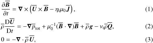
For the analytical study of NEMPI with a vertical field we consider the equations of mean-field MHD for mean magnetic field  , mean velocity
  , and mean density
  in the anelastic approximation for low Mach numbers, and for large fluid and magnetic Reynolds numbers,
 where
where 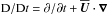 is the advective derivative,
  is the mean total pressure,
  is the mean gas pressure,
 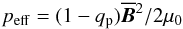 (4)is the effective magnetic pressure (Kleeorin et al. 1990, 1993, 1996), is the mean density,
  is the mean magnetic field with an imposed constant field pointing in the z direction,
  is the mean current density, μ0 is the vacuum permeability, g = (0,0, − g) is the gravitational acceleration, ηt is the turbulent magnetic diffusivity, νt is the turbulent viscosity,
 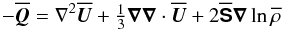 (5)is a term appearing in the viscous force with
 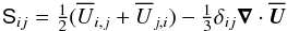 (6)being the traceless rate-of-strain tensor of the mean flow.
We adopt an isothermal equation of state with  , where cs = const. is the sound speed. In the absence of a magnetic field, the hydrostatic equilibrium solution is then given by
  , where
  is the density scale height.
2.1. Analytical estimates of growth rate of NEMPI
We linearize the mean-field Eqs. (1)−(3) around the equilibrium:  ,
,  . The equations for small perturbations (denoted by a tilde) can be rewritten in the form
![Mathematical equation: \begin{eqnarray} &&{\partial \tilde {\bm B}\over \partial t} = \nab \times \left(\tilde {\bm U}\times\meanBB_0 \right), \label{C1}\\ && \nab \cdot \tilde {\bm U} = {\tilde U_z\over H_\rho}, \label{C2}\\ && {\partial \tilde {\bm U}\over \partial t} = {1 \over \meanrho} \left[\mu_0^{-1}(\meanBB_0 \cdot \nab)\tilde {\bm B}- \nab \tilde p_{\rm eff} \right], \label{C3} \end{eqnarray}](/articles/aa/full_html/2014/02/aa22681-13/aa22681-13-eq30.png) where
where 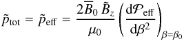 (10)with
  and
and  is the local equipartition field strength, and urms is assumed to be a constant in the present mean-field study. Here, the effective magnetic pressure is written in normalized form as
 ![Mathematical equation: \begin{equation} \Peff(\beta)\equiv \mu_0 p_{\rm eff}/\Beq^2= \half\left[1-\qp(\beta)\right]\beta^2. \end{equation}](/articles/aa/full_html/2014/02/aa22681-13/aa22681-13-eq35.png) (11)In this section, we neglect dissipative terms such as the turbulent viscosity term in the momentum equation and the turbulent magnetic diffusion term in the induction equation. We consider the axisymmetric problem, use cylindrical coordinates r,ϕ,z and introduce the magnetic vector potential and stream function:
(11)In this section, we neglect dissipative terms such as the turbulent viscosity term in the momentum equation and the turbulent magnetic diffusion term in the induction equation. We consider the axisymmetric problem, use cylindrical coordinates r,ϕ,z and introduce the magnetic vector potential and stream function: 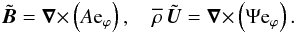 (12)Using the radial component of Eqs. (7) and (9) we arrive at the following equation for the function
  :
: ![Mathematical equation: \begin{equation} {\partial^2 \Phi\over \partial t^2} =v^2_{\rm A}(z) \left[\nabla_z^2 +2 \left({\dd \Peff\over\dd\beta^2} \right)_{\beta=\beta_0} \Delta_{\rm s} \right] \Phi, \label{C6} \end{equation}](/articles/aa/full_html/2014/02/aa22681-13/aa22681-13-eq39.png) (13)where
(13)where  is the mean Alfvén speed, Δs is the radial part of the Stokes operator,
  and we have used an exponential profile for the density stratification in an isothermal layer,
  (14)We seek solutions of Eq. (13) in the form
  (15)where J1(x) is the Bessel function of the first kind, which satisfies the Bessel equation: ΔsJ1(ar) = −a2J1(ar). Substituting Eq. (15) into Eq. (13), we obtain the equation for the function Φ0(z):
 ![Mathematical equation: \begin{equation} {{\rm d}^2\Phi_0 \over {\rm d}z^2} - \left[{\lambda^2 \over v^2_{\rm A}(z)} +{2\sigma^2 \over R^2} \left({\dd \Peff\over\dd\beta^2} \right)_{\beta=\beta_0} \right] \Phi_0 =0. \label{C8} \end{equation}](/articles/aa/full_html/2014/02/aa22681-13/aa22681-13-eq48.png) (16)For
(16)For  , the growth rate of NEMPI is given by
 ![Mathematical equation: \begin{eqnarray} \lambda={v_{\rm A} \sigma \over R} \left[ -2\left(\dd \Peff \over \dd\beta^2 \right)_{\beta=\beta_0}\right]^{1/2} \cdot \label{C10} \end{eqnarray}](/articles/aa/full_html/2014/02/aa22681-13/aa22681-13-eq50.png) (17)This equation shows that, compared to the case of a horizontal magnetic field, where there was a factor Hρ in the denominator, in the case of a vertical field the relevant length is R/σ. Introducing as a new variable
(17)This equation shows that, compared to the case of a horizontal magnetic field, where there was a factor Hρ in the denominator, in the case of a vertical field the relevant length is R/σ. Introducing as a new variable  , we can rewrite Eq. (16) in the form
 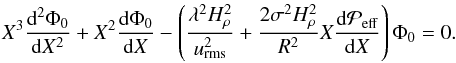 (18)We now need to make detailed assumptions about the functional form of
  . A useful parameterization of qp in Eq. (4) is (Kemel et al. 2012b)
 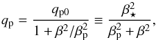 (19)where
  . It is customary to obtain approximate analytic solutions to Eq. (18) as marginally bound states of the associated Schrödinger equation,
  , via the transformation
  , where
 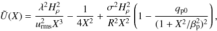 (20)where primes denote a derivative with respect to X. The potential
  has the following asymptotic behavior:
  for small X, and
  for large X. For the existence of an instability, the potential
  should have a negative minimum. However, the exact values of the growth rate of NEMPI, the scale at which the growth rate attains the maximum value, and how the resulting magnetic field structure looks like in the nonlinear saturated regime of NEMPI can only be obtained numerically using MFS.
2.2. MFS models
For consistency with earlier studies, we keep the governing MFS parameters equal to those used in a recent study by Losada et al. (2013). Thus, unless stated otherwise, we use the values  (21)which are based on Eq. (22) of Brandenburg et al. (2012), applied to ReM = 18.
The mean-field equations are solved numerically without making the anelastic approximation, i.e., we solve  (22)together with the equations for the mean vector potential
  such that
  is divergence-free, the mean velocity , and the mean density , using the Pencil Code1, which has a mean-field module built in and is used for calculations both in Cartesian and cylindrical geometries. Here,
  is the imposed uniform vertical field. The respective coordinate systems are (x,y,z) and (r,ϕ,z). In the former case we use periodic boundary conditions in the horizontal directions, − L⊥/2 < (x,y) < L⊥/2, while in the latter we adopt perfect conductor, free-slip boundary conditions at the side walls at r = Lr and regularity conditions on the axis. On the upper and lower boundaries at z = ztop and z = zbot we use in both geometries stress-free conditions,
  and
and  , and assume the magnetic field to be normal to the boundary, i.e.,
  .
.
Following earlier work, we display results for the magnetic field either by normalizing with B0, which is a constant, or by normalizing with Beq, which decreases with height. The strength of the imposed field is often specified in terms of Beq0 = Beq(z = 0).
2.3. Nondimensionalization
Nondimensional parameters are indicated by tildes and hats, and include  and
and  , in addition to parameters in Eq. (21) characterizing the functional form of qp(β). Additional quantities include
  and
and  , where a hat is used to indicate nondimensionalization that uses quantities other than cs and Hρ, such as k1 = 2π/L⊥, which is the lowest horizontal wavenumber in a domain with horizontal extent L⊥. For example,
  , is nondimensional gravity and
  is the nondimensional growth rate. It is convenient to quote also B0/Beq0 with Beq0 = Beq(z = 0). Note that B0/Beq0 is larger than
  by the inverse of the turbulent Mach number, Ma = urms/cs. It is convenient to normalize the mean flow by urms and denote it by a hat, i.e.,
  . Likewise, we define
  .
.
In MFS, the value of ηt is assumed to be given by ηt0 = urms/3kf. Using the test-field method, Sur et al. (2008) found this to be an accurate approximation of ηt. Thus, we have to specify both Ma and  . In most of our runs we use Ma = 0.1 and
  , corresponding to
  . Furthermore, kf and Hρ are in principle not independent of each other either. In fact, mixing length theory suggests kfHρ ≈ 6.5 (Losada et al. 2013), but it would certainly be worthwhile to compute this quantity from high-resolution convection simulations spanning multiple scale heights. However, in this paper, different values of kfHρ are considered. With these preparations in place, we can now address questions concerning the horizontal wavelength of the instability and the vertical structure of the magnetic flux tubes.
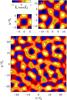 |
Fig. 1 Horizontal patterns of |
2.4. Aspect ratio of NEMPI
The only natural length scale in an isothermal layer in MFS is Hρ. It determines the scale of NEMPI. At onset, the horizontal scale of the magnetic field pattern will be a certain multiple of Hρ. In the following we denote the corresponding horizontal wavenumber of this pattern by k⊥. Earlier work by Kemel et al. (2013) showed that for an imposed horizontal magnetic field we have k⊥Hρ ≈ 0.8...1. This pattern was 2D in the plane perpendicular to the direction of the imposed magnetic field, corresponding to horizontal rolls oriented along the mean magnetic field. In the present case of a vertical field, the magnetic perturbations have a cellular pattern with horizontal wavenumber k⊥. To determine the value of k⊥Hρ for the case of an imposed vertical magnetic field, we have to ensure that the number of cells per unit area is independent of the size of the domain. In Fig. 1, we compare MFS with horizontal aspect ratios ranging from 2 to 8. We see that the magnetic pattern is fully captured in a domain with normalized horizontal extent L⊥/Hρ = 4π, i.e., the horizontal scale of the magnetic field pattern is twice the value of Hρ, i.e.,  , so that
  , or k⊥Hρ ≈ 0.7. The value k⊥Hρ ≈ 0.7 is also confirmed by taking a power spectrum of
  ; see Fig. 2, which shows a peak at a similar value.
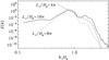 |
Fig. 2 Power spectra of |
Comparing the three simulations shown in Fig. 1, we see that a regular checkerboard pattern is only obtained for the smallest domain size; see Fig. 1a. For larger domain sizes the patterns are always irregular such that a cell of one sign can be surrounded by 3–5 cells of the opposite sign. Nevertheless, in all three cases we have approximately the same number of cells per unit area.
In the nonlinear regime, structures continue to merge and more power is transferred to lower horizontal wavenumbers; see Fig. 3. Later in Sect. 3.5 we present similar results also for our DNS.
2.5. Vertical magnetic field profile during saturation
In an isothermal atmosphere, the scale height is constant and there is no physical upper boundary, so we can extend the computation in the z direction at will, although the magnetic pressure will strongly exceed the turbulent pressure at large heights, which can pose computational difficulties. To study the full extent of magnetic flux concentrations, we need a big enough domain. In the following we consider the range − 3π ≤ z/Hρ ≤ 3π, which results in a density contrast of more than 108. To simplify matters, we restrict ourselves in the present study to axisymmetric calculations which are faster than 3D Cartesian ones.
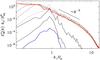 |
Fig. 3 Time evolution of normalized spectra of Bz from 3D MFS during the late nonlinear phase at the top of the domain, k1z = π, at normalized times |


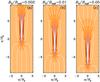 |
Fig. 4 Comparison of magnetic field profiles from axisymmetric MFS for Runs Bv002/33–Bv05/33 with three values of B0/Beq0 and |
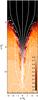 |
Fig. 5
|
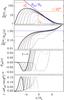 |
Fig. 6 Time evolution of normalized vertical magnetic field profiles, a) |

In Fig. 4 we compare the results for the mean magnetic field profiles for three values of B0/Beq0 ranging from 0.002 to 0.05. These values are smaller than those studied in Sect. 2.4, because in the nonlinear regime and in a deeper domain the structures are allowed to sink by a substantial amount. By choosing B0/Beq0 to be smaller, the tubes are fully contained in our domain. As B0 increases, we expect the position of the magnetic flux tube, zB, to move downward like 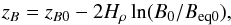 (23)where
  is a reference height and
 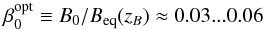 (24)is the optimal normalized field strength for NEMPI to be excited (Losada et al. 2013). The validity of Eq. (23) can be verified through Fig. 4, where B0/Beq0 increases by a factor of 25, corresponding to ΔzB = −6.4.
In all cases, we obtain a slender tube with approximate aspect ratio of 1:8. In other words, the shape of the magnetic field lines is the same for all three values of B0/Beq0, and just the position of the magnetic flux concentration shifts in the vertical direction. Note in particular that the thickness of structures is always the same. This is different from the nonlinear MFS in Cartesian geometry discussed above, where structures are able to merge. Merging is not really possible in the same way in an axisymmetric container, because any additional structure would correspond to a ring.
The mean flow structure associated with the magnetic flux tube is shown in Fig. 5 for Run Bv05/33 with B0/Beq0 = 0.05. We find inflow into the tube along field lines at large heights and outflow at larger depth. The vertical component of the flow in the tube points always downward, i.e., there is no obvious effect from positive magnetic buoyancy. The maximum downflow speed is about 0.27urms, so it is subdominant compared with the turbulent velocity, but this could be enough to cause a noticeable temperature change in situations where the energy equation is solved.
The resulting magnetic field lines look roughly similar to those of the DNS with an imposed vertical magnetic field (Brandenburg et al. 2013). In DNS, however, the thickness of the magnetic flux tube is larger than in the MFS by about a factor of three. This discrepancy could be explained if the actual value of ηt was in fact larger than the estimate given by ηt0. We return to this possibility in Sect. 3.5. Alternatively, it might be related to the possibility that the coefficients in Eq. (21) could actually be different.
The time evolution of the vertical magnetic field profiles,  and
and  , is shown in Fig. 6 at different times for the case B0/Beq0 = 0.05, corresponding to Fig. 4c. Here, we also show the time evolution of the corresponding profiles of
  and
and  . In the kinematic regime, the peak of the latter quantity is a good indicator of the peak of the eigenfunction (Kemel et al. 2013). In the present case, the magnetic field in the kinematic phase peaks at a height zB that is given by the condition (24). According to the MFS of Losada et al. (2013), this condition is approximately the same for vertical and horizontal fields. Looking at Fig. 6 for B0/Beq0 = 0.05, we see that at z/Hρ ≈ − 0.5 we have Beq/B0 ≈ 33, which agrees with Eq. (24). However, unlike the case of a horizontal magnetic field, where in the kinematic phase the mean field was found to peak at a height below that where peaks, we now see that the field peaks above that position.
As NEMPI begins to saturate, the peak of  moves further down to
  during the next one or two turbulent diffusive times. By that time, has reached values up to
  . At that depth,
  is about 0.25, but this quantity continues to increase with height and reaches super-equipartition values at z/Hρ ≈ 3 (second panel of Fig. 6).
2.6. Smaller scale separation
 |
Fig. 7 Comparison of magnetic field profiles from an axisymmetric MFS for Runs Bv01/33–Bv01/7 with B0/Beq0 = 0.01 and three values of kfHρ. |
In MFS, as noted above, the wavenumber of turbulent eddies, kf, enters the expression for the turbulent diffusivity via ηt ≈ urms/3kf, and thus  , so we have
 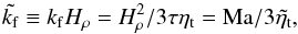 (25)where τ = Hρ/urms is the turnover time per scale height. When urms is kept unchanged, smaller scale separation implies a decrease of , i.e., the size of turbulent eddies in the domain is increased. Earlier work has indicated that the growth rate of the instability for horizontal magnetic field decreases with decreasing (Brandenburg et al. 2012). However, we do not know whether this also causes a change in the spot diameter, which would be plausible, or a change in the depth at which NEMPI occurs. In our MFS we have chosen Ma = 0.1 and
  corresponds to
  . For
. For  we have
  , which is about the smallest scale separation for which NEMPI is still possible in this geometry; see Fig. 7. Interestingly, as is decreased, the location of the flux tube structure moves upward. This can be understood as a consequence of enhanced turbulent diffusion, which makes the flux tubes less concentrated, so the magnetic field is weaker, but weaker magnetic field sinks less than stronger fields.
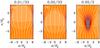 |
Fig. 8 Comparison of magnetic field structure in axisymmetric MFS. a) Run 0.01/33 with B0/Beq0 = 0.01 and b) Run 0.05/33 with B0/Beq0 = 0.05, both with kfHρ = 33. The flow speeds vary from − 0.27urms to 0.08urms in both cases. c) Run 0.05/3 with B0/Beq0 = 0.05 and kfHρ = 3. The flow speed varies from − 0.23urms to 0.07urms. |
Even for kfHρ ≈ 3 it is still possible to find NEMPI in MFS, but, as we have seen, the flux tube moves upward and becomes thicker. To accommodate for this change, we need to increase the diameter of the domain and, in addition, we would either need to extend it in the upward direction or increase the magnetic field strength to move the tube back down again; cf. Fig. 4. We choose here the latter. In Fig. 8, we show three cases for a wider box. In the first two runs (referred to as “0.01/33” and “0.05/33”) we keep the scale separation ratio the same as before, i.e. , and increase B0/Beq0 from 0.01 to 0.05, while in the third case we keep B0/Beq0 = 0.05 and decrease to 3. We increase the magnetic field by a factor of 5 so as to keep the structure within the computational domain. In the first case, the natural separation between tubes would be too small for this large cylindrically symmetric container. By contrast, in a 3D Cartesian domain, a second downdraft would form, which is not possible in an axisymmetric geometry. Instead, a downdraft develops on the outer rim of the container. On the other hand, if is decreased and thus increased, a single downdraft is again possible, as shown in Fig. 8b, suggesting that the horizontal scale of structures is also increased as is increased. We see that the tube can now attain significant diameters. Its height remains unchanged, so the aspect ratio of the structure is decreased as the scale separation ratio is decreased.
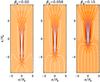 |
Fig. 9 Comparison of magnetic field structure in axisymmetric MFS for Runs Bu01/33–Bw01/33 with three values of βp. |
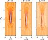 |
Fig. 10 Comparison of magnetic field structure in axisymmetric MFS for Runs Av01/33–Cv01/33 three values of β⋆. |
Survey of axisymmetric MFS giving normalized growth rates, mean field strengths, mean flow speeds, and other properties for different values of β0, β⋆, βp, and .
2.7. Parameter sensitivity
It is important to know the dependence of the solutions on changes of the parameters βp and β⋆ that determine the function qp. In Figs. 9 and 10, we present results where we change either βp or β⋆, respectively. Characteristic properties of these solutions are summarized in Table 1. Runs Ov002/33–Ov05/33 are 2D Cartesian while all other ones are 2D axisymmetric. In addition to βp and β⋆, we also list the values of  , as well as the minimum position of the
  curve, namely (cf. Kemel et al. 2012b)
 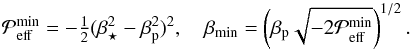 (26)The main output parameters include the normalized growth rate in the linear regime,
  , the maximum normalized vertical field in the tube
  (27)the minimum and maximum normalized velocities,
 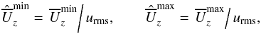 (28)the normalized maximum magnetic field positions in the linear and nonlinear regimes,
  and
and  , respectively, the similarly normalized positions where
  has dropped by 1/e of its maximum at the bottom end
  , at the top end
  , and to the side
  of the tube, as well as the aspect ratio A = Zt/R.
The changes of  are often as expected: a decrease with decreasing values of , and a increase with increasing values of β⋆. There are also some unexpected changes that could be associated with the tube not being fully contained within our fixed domain: for Run Ov05/33 the domain may not be deep enough and for Run Bw01/33 it may not be wide enough. Furthermore, we find that structures become taller when βp is small and β⋆ large, and they become shorter and fatter when βp is large and β⋆ small. Thus, thicker structures, as indicated by the DNS of Brandenburg et al. (2013), could also be caused by larger values of βp or smaller values of β⋆. When the domain is clipped at z = 0, flux concentrations cannot fully develop. The structures are fatter and less strong; see Fig. 11.
 |
Fig. 11 Comparison of magnetic field structure in axisymmetric MFS for Runs Av–Cv01/33* with three values of β⋆ in a domain that is truncated from below. |
2.8. Effect of rotation
The effect of rotation through the Coriolis force is determined by the Coriolis number, 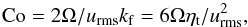 (29)where Ω is the angular velocity. Losada et al. (2012, 2013) found that NEMPI begins to be suppressed when Co ≳ 0.03, which is a surprisingly small value. They only considered the case of a horizontal magnetic field. In the present case of a vertical magnetic field, we can use the axisymmetric model to include a vertical rotation vector Ω = (0,0,Ω). We add the Coriolis force to the right-hand side of Eq. (2), i.e.,
  (30)When adding weak rotation (Co = 0.01) in Run Bv01/33, it turns out that magnetic flux concentrations develop on the periphery of the domain, similar to the case considered in Fig. 8. We have therefore reduced the radial extent of the domain to r/Hρ ≤ π/2. The results are shown in Fig. 12.
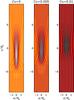 |
Fig. 12 Comparison of magnetic field structure in axisymmetric MFS for a run similar to Run Bv01/33, but for three values of Co and r/Hρ ≤ π/2. |
In agreement with earlier studies, we find that rather weak rotation suppresses NEMPI. The magnetic structures become fatter and occur slightly higher up in the domain. For Co = 0.01, the magnetic flux concentrations have become rather weak. If we write Co in terms of correlation of turnover time τ as 2Ωτ, we find that the solar values of Ω = 3 × 10⁻⁶ s-1 corresponds to 30min. According to stellar mixing length theory, this, in turn, corresponds to a depth of less than 2 Mm.
3. DNS and ILES studies
In the MFS discussed above, we have ignored the possibility of other terms in the parameterization of the mean-field Lorentz force. While this seems to capture the essence of earlier DNS (Brandenburg et al. 2013), this parameterization might not be accurate or sufficient in all respects. It is therefore useful to perform DNS to see how the results depend on scale separation, gravitational stratification, and Mach number.
3.1. DNS and ILES models
We have performed direct numerical simulations using both the Pencil Code2 and Nirvana3. Both codes are fully compressible and are here used with an isothermal equation of state with , where cs = const is the sound speed. The background stratification is then also isothermal. Turbulence is driven using volume forcing given by a function f that is δ-correlated in time and monochromatic in space. It consists of random non-polarized waves whose direction and phase change randomly at each time step.
In DNS we solve the equations for the velocity U, the magnetic vector potential A, and the density ρ, 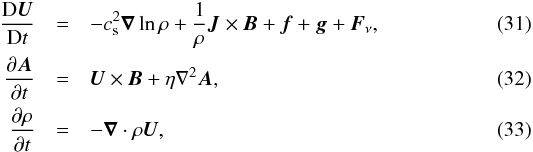 where D/Dt = ∂/∂t + U·∇ is the advective derivative, η is the magnetic diffusivity due to Spitzer conductivity of the plasma,
  is the magnetic field, is the imposed uniform vertical field, J = ∇ × B/μ0 is the current density, μ0 is the vacuum permeability,
  is the viscous force. The turbulent rms velocity is approximately independent of z. Boundary conditions are periodic in the horizontal directions (so vertical magnetic flux is conserved), and stress free on the upper and lower boundaries, where the magnetic field is assumed to be vertical, i.e., Bx = By = 0. In the ILES we solve the induction equation directly for B, ignore the effects of explicit viscosity and magnetic diffusivity and use an approximate Riemann solver to keep the code stable and to dissipate kinetic and magnetic energies at small scales.
The simulations are characterized by specifying a forcing amplitude, which results in a certain rms velocity, urms, and hence in a certain Mach number. Furthermore, the values of ν and η are quantified through the fluid and magnetic Reynolds numbers, Re = urms/νkf and ReM = urms/ηkf, respectively. Their ratio is the magnetic Prandtl number, PrM = ν/η. Occasionally, we also quote  and
and  .
.
An important diagnostics is the vertical magnetic field, Bz, at some horizontal layer. In particular, we use here the Fourier-filtered field, , which is obtained by removing all components with wavenumbers larger than 1/6 of the forcing wavenumber kf. This corresponds to a position in the magnetic energy spectrum where there is a local minimum, so we have some degree of scale separation between the forcing scale and the scale of the spot. We return to this in Sect. 3.5. To identify the magnetic field in the flux tube, we take the maximum of , either at each height at one time, which is referred to as  , or in the top layer at different times. The latter is used to determine the growth rate of the instability.
When comparing results for different values of g, it is convenient to keep the typical density at the surface the same. Since our hydrostatic stratification is given by Eq. (14), this is best done by letting the domain terminate at z = 0 and to consider the range − Lz ≤ z ≤ 0. In most of the cases we consider Lz = π/k1, although this might in hindsight be a bit short in some cases. For comparison with earlier work of Brandenburg et al. (2013), we also present models in a domain − π ≤ k1z ≤ π.
Summary of DNS at varying , and fixed values of  , PrM = 0.5, Re ≈ 38, Ma ≈ 0.1, ĝ = 1,
  , τtd/τto ≈ 2700, using 2563 mesh points.
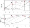 |
Fig. 13 Normalized vertical magnetic field profiles from DNS, |

3.2. Magnetic field dependence
In Table 2 and Fig. 13 we compare results for six values of 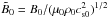 . These models are the same as those discussed in Brandenburg et al. (2013), where visualizations are shown for all six cases. Increasing leads to a decrease in the Mach number Ma and hence to a mild decline of Re and ReM for
  , corresponding to B0/Beq0 > 0.1. There is a slight increase of
  , while
  remains on the order of unity. This is the case even for the largest value,
  , when NEMPI is completely suppressed and there is no distinct maximum of
  in the upper panel of Fig. 13. This is why the visualization in Brandenburg et al. (2013) was featureless for , even though
  at z = ztop. Moreover, while shows only a slight increase, the non-dimensional radius of the spot increases from 0.1 to about 0.4 as is increased.
Summary of DNS at varying PrM, and fixed values of ,  , ReM ≈ 20–40, Ma ≈ 0.1, ĝ = 1, , τtd/τto ≈ 2700, using 2563 mesh points.
Summary of DNS at varying Re and ReM, and fixed values of  , , PrM = 0.5, k1Hρ = 1, and kfHρ = 30.
3.3. Magnetic Prandtl number dependence
The results for different values of PrM are summarized in Table 3. It turns out that for PrM ≥ 5, no magnetic flux concentrations are produced. We recall that analysis based on the quasi-linear approach (which is valid for small fluid and magnetic Reynolds numbers) has shown that for PrM ≥ 8 and ReM ≪ 1, no negative effective magnetic pressure is possible (Rüdiger et al. 2012; Brandenburg et al. 2012). Because of this, most of the earlier work used PrM = 0.5 so as to stay below unity in the hope that this would be a good compromise between PrM being small and ReM still being reasonably large. In fact, it now turns out that the difference in for PrM = 1 and 1/2 be negligible, and even for PrM = 2 the decline in is still small. For PrM = 0.2, on the other hand, we find a large value of , but a low saturation level. Again, this might be explained by the fact that the domain is not deep enough in the z direction, which can suppress NEMPI. Alternatively, the resolution of 2563 might not be sufficient to resolve the longer inertial range for smaller magnetic Prandtl numbers. In Sect. 3.4 we present another case with PrM = 0.2 where both the resolution and the Reynolds numbers are doubled, and is again large.
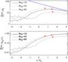 |
Fig. 14 Similar to Fig. 13, but for DNS Runs A30/1–C30/1 listed in Table 4, i.e., |
3.4. Reynolds number dependence
Increasing ReM from 19 to 95, we see some changes; see Table 4. There is first a small increase of from 0.87 to 1.02 as ReM is increased from 19 to 40 (Run B30/1). Increasing Re to 200, but keeping ReM = 40, results in a further increase of to 1.10 (Run b30/1). This is also an example of a strong flux concentration with PrM = 0.2; cf. Sect. 3.3. However, when ReM is increased further to 95, decreases to about 0.71; see Table 4. Again, the weakening of the spot might be a consequence of the domain not being deep enough. Alternatively, it could be related to the occurrence of small-scale dynamo action, which is indicated by the fact that in deeper layers the small-scale magnetic field is enhanced in the run with the largest value of ReM; see Fig. 14. In Run C30/1 with the largest value of ReM, the spot is larger and more fragmented, but it still remains in place and statistically steady; see Fig. 15 and online material4 for corresponding animations.
To eliminate the possibility of the domain not being deep enough, we have performed additional simulations where we have extended the domain in the negative z direction down to zbot/Hρ = −1.5π. In Fig. 16 we show a computation of the resulting profiles of and . We also include here a run with PrM = 1 instead of 0.5 (Run E30/1). It turns out that the strength of the spot is unaffected by the position of zbot and that there is a deep layer below z/Hρ ≈ − 2 in which there is significant magnetic field generation owing to small-scale dynamo action, preventing thereby also the value of to drop below the desired value of 0.01. This might explain the weakening of the spot. This is consistent with earlier analytical (Rogachevskii & Kleeorin 2007) and numerical (Brandenburg et al. 2012) work showing a finite drop of the important NEMPI parameter β⋆ around ReM = 60.
 |
Fig. 15 Magnetic field configuration at the upper surface for DNS Runs A30/1–C30/1 at three values of the magnetic Reynolds number. The white contours represent the Fourier-filtered with k⊥ ≤ kf/6; their levels correspond to |
Summary of DNS at varying , , , and fixed values of ,  , using resolutions of 2563 mesh points (for Run a30/1), 5123 mesh points (for Run a30/4, a10/3, and a30/3), as well as 10242 × 384 mesh points (for Runs a40/1 and A40/1).
3.5. Dependence on scale separation and stratification
We have performed various sets of additional simulations where we change ĝ and/or  ; see Table 5 and Fig. 17. In those cases, the vertical extent of the domain is from − π to 0. As discussed in Sect. 3.1 this might be too small in some cases for NEMPI to develop fully. Nevertheless, in all cases there are clear indications for the occurrence of flux concentrations. The results regarding the growth rate of NEMPI are not fully conclusive, because the changes in kf and Hρ also affect turbulent-diffusive and turnover time scales. As shown in the appendix of Kemel et al. (2013) the normalized growth rate of NEMPI is given by:
 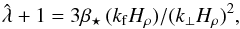 (34)which is not changed significantly for a vertical magnetic field; see Sect. 2.1. If k⊥Hρ = const. ≈ 0.7, as suggested by the MFS of Sect. 2.4, we would expect
  to be proportional to kfHρ, which is not in good agreement with the simulation results.
To shed some light on this, we now discuss horizontal power spectra of Bz(x,y) taken at the top of the domain. These spectra are referred to as  and are normalized by
  . In Run a30/4 with ĝ = 4 and , we have access to wavenumbers down to k1Hρ = 0.25. The results in Fig. 18 show that there is significant power below k⊥Hρ = 0.7. This is in agreement with the MFS in the nonlinear regime; see Fig. 3. The time evolution of suggest a behavior similar to that of an inverse magnetic helicity cascade that was originally predicted by (Frisch et al. 1975) and later verified both in closure calculations (Pouquet et al. 1976) and DNS (Brandenburg 2001). Similar results with inverse spectral transfer are shown in Fig. 19 for DNS Run A40/1. The only difference between Runs A40/1 and a40/1 is the vertical extent of the domain, which is twice as tall in the former case (3πHρ instead of 1.5πHρ). We note in this connection that the spectra tend to show a local minimum near kf/6. This justifies our earlier assumption of separating mean and fluctuating fields at the wavenumber kf/6; see Sect. 3.1. The spectra also show something like an inertial subrange proportional to k− 5/3 (Fig. 19) or k-2.5 (Fig. 18). The latter is close to the k-3 subrange in the MFS of Fig. 3. Those steeper spectra could be a symptom of a low Reynolds number or, alternatively, a consequence of most of the energy inversely “cascading” to larger scales in the latter two cases.
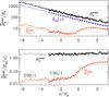 |
Fig. 16 Similar to Fig. 14, but for DNS Runs C30/1 (zbot/Hρ = −π; thicker lines) and D30/1 (zbot/Hρ = −1.5π; thinner lines) listed in Table 4, i.e., |
We have also checked how different kinds of helicities vary during NEMPI. In the present case, magnetic and kinetic helicities are fluctuating around zero, but cross helicity is not. The latter is an ideal invariant of the magnetohydrodynamic (MHD) equations, but in the present case of a stratified layer with a vertical net magnetic field, ⟨u·b⟩ can actually be produced; see Rüdiger et al. (2011), who showed that 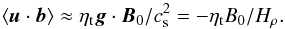 (35)In a particular case of Run 30/1, we find a time-averaged value of ⟨u·b⟩ that would suggest that ηt/ηt0 is around 6, which is significantly larger than unity. This would agree with independent arguments in favor of having underestimated ηt; see the discussion in Sect. 2.5. In other words, if ηt were really larger than what is estimated based on the actual rms velocity, it would also explain why the diameter of tubes is bigger in the DNS than in the MFS.
Summary of DNS and ILES at varying values of Ma, all for ĝ = 3,  .
.
3.6. Mach number dependence
To study the dependence on Mach number, it is useful to consider ILES without any explicit viscosity or magnetic diffusivity. In Figs. 20−22 we show the results for three values of Ma at  and using a resolution of 2562 × 128 nodes on the mesh. In Table 6 we give a summary of various output parameters and compare with corresponding DNS. Note first of all that the results from ILES are generally in good agreement with the DNS. This demonstrates that the mechanism causing magnetic flux concentrations by NEMPI is robust and not sensitive to details of the magnetic Reynolds number, provided that ReM ≳ 10. The normalized growth rate is in all three cases above unity.
As the Mach number is increased, the magnetic structures become smaller; seen in the left-hand panels of Fig. 22. Since the properties of NEMPI depend critically on the ratio  , and since Beq(z) and hence Beq0 increase with increasing Mach number, the decrease in the size of magnetic structures might just reflect the fact that for smaller values of
  , NEMPI would operate at higher layers which are no longer included in our computational domain. Looking at Fig. 20, it is clear that the maximum of
  moves to higher layers, but it is still well confined within the computational domain. Nevertheless, if one compensates for the decrease of Beq by applying successively weaker mean fields when going to lower Mach number (right-hand panels of Fig. 22), the size of the emerging structures remains approximately similar and the curves of lie now nearly on top of each other. This shows clearly that in our simulations with Ma ≈ 0.7, flux concentrations are well possible. This is important, because it allows for the possibility that the energy density of magnetic flux concentrations can become comparable with the thermal energy.
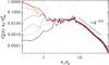 |
Fig. 18 Normalized spectra of Bz from DNS Run a30/4 at normalized times |


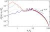 |
Fig. 19 Normalized spectra of Bz from DNS Run A40/1 at normalized times |
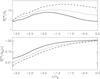 |
Fig. 20 Same as Fig. 13, but for the ILES runs with varying forcing amplitude. Note the different vertical extent of this set of models. The different lines indicate Ma = 0.16 (solid), 0.34 (dotted), and 0.68 (dashed). |
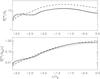 |
Fig. 21 Same as Fig. 20, but for the ILES runs which vary both the forcing amplitude and the imposed magnetic field at the same time, keeping the relative field strength comparable. The different lines again indicate Ma = 0.16 (solid), 0.35 (dotted), and 0.68 (dashed), and agree markedly well in the lower panel where we plot relative to Beq(z). |
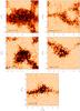 |
Fig. 22 Surface appearance of the vertical magnetic field, |


4. Possible application to sunspot formation
Compared with earlier studies of NEMPI using a horizontal imposed magnetic field, the prospects of applying it to the Sun have improved in the sense that the flux concentrations are now stronger when there is a vertical magnetic field. In particular, the resulting magnetic structures survive in the presence of larger Mach numbers up to 0.7, which is relevant to the photospheric layers of the Sun (Stein & Nordlund 1998). However, those structures do become somewhat weaker as the magnetic Reynolds number is increased sufficiently to allow for the presence of small-scale dynamo action. This was expected based on a certain drop of β⋆ for ReM ≳ 60 found in earlier simulations (Brandenburg et al. 2012), but the possibility of spot formation still persists. More specifically, we have seen that the largest field strength, , occurs at a height where  is at least 0.4; see Fig. 16.
To speculate further regarding the applicability to sunspot formation, we must look at the mean-field models presented in Sect. 2. In particular, we have seen that spot formation occurs at a depth  where is between 0.6 (for ReM = 40) and 0.4 (for ReM = 95); see Fig. 14 and Table 4. Larger ratios of occur in the upper layers, but then the absolute field strength is lower. In the MFS of Sect. 2, the value of at
  is somewhat smaller (around 0.3), suggesting that the adopted set of mean-field parameters in Eq. (21) was slightly suboptimal. Nevertheless, those models show that the depth where NEMPI occurs and where the effective magnetic pressure is most negative is even further down, e.g., at z/Hρ ≈ − 7; see Fig. 5. Furthermore, at the depth where is maximum, i.e., where NEMPI is strongest according to theory, we find
  . Thus, there is an almost tenfold increase of the absolute field strength between the depth were NEMPI occurs and where the field is strongest.
As we have seen from Fig. 5, this increase is caused solely by hydraulic effects, similar to what Parker (1976, 1978) anticipated over 35 years ago. Our isothermal models clearly do demonstrate the hydraulic effect due to downward suction, but we cannot expect realistic estimates for the resulting field amplification. Parker (1978) gives more realistic estimates, but in his work the source of downward flows remained unclear. Our present work suggests that NEMPI might drive such motion, but in realistic simulations it would be harder to identify this as the sole mechanism. Another mechanism might simply be large-scale hydrodynamic convection flows that would continue deeper down to the lower part of the supergranulation layer at depths between 20 and 40 Mm. Some indications of this have now been seen in simulations of Stein & Nordlund (2012). Whether the reason for flux concentrations is then NEMPI or convection can only be determined through careful numerical experiments comparing full MHD with the case of a passive vector field. Such a field would still be advected by convective flows but would not contribute to the dynamical effects that would be required if NEMPI were to be responsible.
In addition to the magnetic field strength of flux concentrations, there might also be issues concerning their size. Usually they are not much larger than about 5 density scale heights; see, e.g., Fig. 15. This might be too small to explain sunspots. On the other hand, in the supergranulation layer, the density scale height increases, and larger scale structures might be produced at those depths.
To make this more concrete, let us discuss a possible scenario. At a depth of 3 Mm, the equipartition field strength is about 2 kG, and this might be where the sunspot field is strongest. If NEMPI was to be responsible for this, we should expect the effective magnetic pressure to be negative at a depth of about 10 Mm. Here, the equipartition field strength is about 3 kG. If NEMPI operates at  , this would correspond to
  , which appears plausible. At that depth, the density scale height is also about 10 Mm. Thus, if magnetic flux concentrations have a size of 5 density scale heights, then this would correspond to 50 Mm at that depth. To produce spots higher up, the field would need to be more concentrated, which would reduce the size by a factor of 3 again. However, given the many uncertainties, it is impossible to draw any further conclusions until NEMPI has been studied under more realistic conditions relevant to the Sun.
5. Conclusions
Using DNS, ILES and MFS in a wide range of parameters we have demonstrated that an initially uniform vertical weak magnetic field in strongly stratified MHD turbulence with large scale separation results in the formation of circular magnetic spots of equipartition and super-equipartition field strengths. Although we have confirmed that the normalized horizontal wavenumber of magnetic flux concentrations is k⊥Hρ ≈ 0.8, as found earlier for horizontal imposed field (Kemel et al. 2013), it is now clear that in the nonlinear regime smaller values can be attained. This happens in a fashion reminiscent of an inverse cascade or inverse transfer5 in helically forced turbulence (Brandenburg 2001). In the present case, this inverse transfer is found both in MFS and in DNS. This property helps explaining the possibility of larger length scales separating different flux concentrations.
The study of axisymmetric MFS helps understanding the dependence of NEMPI on the parameters β⋆ and βp, which determine the parameterization of the effective magnetic pressure, . It was always clear that changes in those parameters can significantly change the functional form of , and yet the resulting growth rate of NEMPI was found to depend mainly on the value of β⋆. We now see, however, that the shape of the resulting solutions still depends on the value of βp, in addition to a dependence on β⋆. In fact, smaller values of βp as well as larger values of β⋆ both result in longer structures. This is important background information in attempts to find flux concentrations in DNS, where the domain might not always be tall enough. As a rule of thumb, we can now say that the domain is deep enough if the resulting large-scale magnetic field is below 1% of the equipartition value. This is confirmed by Figs. 13 and 14 as well as Figs. 20 and 21, where all runs with  at z = zbot reach
  at z = ztop, provided the domain is also high enough. A limited extent at the top appears to be less critical than at the bottom, because NEMPI still develops in almost the same way as before.
It is important to emphasize that the formation of magnetic flux concentrations is equally well possible at large Mach numbers. This is important in view of applications to the Sun, where in the upper layers Ma ≈ 0.5 can be expected. Nevertheless, our present investigations have not yet been able to address the question whether sunspots can really form through NEMPI. For that, we would need to abandon the assumption of isothermality. Nevertheless, we expect the basic feature of downflows along flux tubes to persist also in that case. It is the associated inflow from the side that keeps the tube concentrated. Such flows have indeed been seen in local helioseismology (Zhao et al. 2010). Those authors also find an additional outflow higher in the photosphere that is known as the Evershed flow.
We expect that the downflow in the tube plays an important role in an unstably stratified layer, such as in the Sun, where it brings low entropy material to deeper layers, lowering therefore the effective temperature in the magnetic tubes. Future work should hopefully be able to demonstrate that in detail. The conceptual difference between NEMPI and other mechanisms may not always be very clear. However, by using an isothermal layer, we can be sure that convection is not operating. Thus, the phenomenon of flux segregation found by Tao et al. (1998) would not work. Conversely, however, NEMPI might well be a viable explanation for this phenomenon too. Whether the concept of flux expulsion can really serve as an alternative paradigm is unclear, because it is difficult to draw any quantitative predictions from it. In particular, flux expulsion does not make any reference to turbulent pressure or its suppression. Instead, the source of free energy is more directly potential energy which can be tapped through the superadiabatic gradient in convection. By contrast, the source of free energy for NEMPI is turbulent energy. The other possibility discussed above is the network of downdrafts associated with the supergranulation layer (Stein & Nordlund 2012). This mechanism is not easily disentangled from NEMPI, because both imply flux concentrations in downdrafts. However, in an isothermal layer, we can be sure that supergranulation flows are absent, so NEMPI is the only known mechanism able to explain the flux concentrations shown in the present paper.
In both cases, the transfer is nonlocal in wavenumber space. It is therefore more appropriate to use the term inverse transfer instead of inverse cascade.
Acknowledgments
This work was supported in part by the European Research Council under the AstroDyn Research Project No. 227952, by the Swedish Research Council under the project grants 2012-5797 and 621-2011-5076 (AB), by the European Research Council under the Atmospheric Research Project No. 227915, and by a grant from the Government of the Russian Federation under contract No. 11.G34.31.0048 (NK, IR). We acknowledge the allocation of computing resources provided by the Swedish National Allocations Committee at the Center for Parallel Computers at the Royal Institute of Technology in Stockholm and the National Supercomputer Centers in Linköping, the High Performance Computing Center North in Umeå, and the Nordic High Performance Computing Center in Reykjavik. Part of this work used the Nirvana code version 3.3, developed by Udo Ziegler at the Leibniz-Institut für Astrophysik Potsdam (AIP).
References
- Biskamp, D. 1993, Nonlinear magnetohydrodynamics (Cambridge: Cambridge University Press) [Google Scholar]
- Brandenburg, A. 2001, ApJ, 550, 824 [NASA ADS] [CrossRef] [Google Scholar]
- Brandenburg, A. 2005, ApJ, 625, 539 [Google Scholar]
- Brandenburg, A., Kemel, K., Kleeorin, N., Mitra, D., & Rogachevskii, I. 2011, ApJ, 740, L50 [NASA ADS] [CrossRef] [Google Scholar]
- Brandenburg, A., Kemel, K., Kleeorin, N., Rogachevskii, I. 2012, ApJ, 749, 179 [NASA ADS] [CrossRef] [Google Scholar]
- Brandenburg, A., Kleeorin, N., & Rogachevskii, I. 2013, ApJ, 776, L23 [NASA ADS] [CrossRef] [Google Scholar]
- Cheung, M. C. M., Rempel, M., Title, A. M., & Schüssler, M. 2010, ApJ, 720, 233 [NASA ADS] [CrossRef] [Google Scholar]
- Fan, Y. 2009, Liv. Rev. Sol. Phys., 6, 4 [Google Scholar]
- Frisch, U., Pouquet, A., Léorat, J., & Mazure, A. 1975, J. Fluid Mech., 68, 769 [NASA ADS] [CrossRef] [Google Scholar]
- Grinstein, F. F., Fureby, C., & DeVore, C. R. 2005, Int. J. Num. Meth. Fluids, 47, 1043 [CrossRef] [Google Scholar]
- Kemel, K., Brandenburg, A., Kleeorin, N., Mitra, D., & Rogachevskii, I. 2012a, Sol. Phys., 280, 321 [NASA ADS] [CrossRef] [Google Scholar]
- Kemel, K., Brandenburg, A., Kleeorin, N., & Rogachevskii, I. 2012b, Astron. Nachr., 333, 95 [NASA ADS] [CrossRef] [Google Scholar]
- Kemel, K., Brandenburg, A., Kleeorin, N., Mitra, D., & Rogachevskii, I. 2013, Sol. Phys., 287, 293 [NASA ADS] [CrossRef] [Google Scholar]
- Kitiashvili, I. N., Kosovichev, A. G., Wray, A. A., & Mansour, N. N. 2010, ApJ, 719, 307 [NASA ADS] [CrossRef] [Google Scholar]
- Kleeorin, N., & Rogachevskii, I. 1994, Phys. Rev. E, 50, 2716 [NASA ADS] [CrossRef] [Google Scholar]
- Kleeorin, N. I., Rogachevskii, I. V., & Ruzmaikin, A. A. 1989, Sov. Astron. Lett., 15, 274 [NASA ADS] [Google Scholar]
- Kleeorin, N. I., Rogachevskii, I. V., & Ruzmaikin, A. A. 1990, Sov. Phys. JETP, 70, 878 [Google Scholar]
- Kleeorin, N., Mond, M., & Rogachevskii, I. 1993, Phys. Fluids B, 5, 4128 [NASA ADS] [CrossRef] [Google Scholar]
- Kleeorin, N., Mond, M., & Rogachevskii, I. 1996, A&A, 307, 293 [NASA ADS] [Google Scholar]
- Losada, I. R., Brandenburg, A., Kleeorin, N., Mitra, D., & Rogachevskii, I. 2012, A&A, 548, A49 [NASA ADS] [CrossRef] [EDP Sciences] [Google Scholar]
- Losada, I. R., Brandenburg, A., Kleeorin, N., & Rogachevskii, I. 2013, A&A, 556, A83 [NASA ADS] [CrossRef] [EDP Sciences] [Google Scholar]
- Parker, E. N. 1976, ApJ, 210, 816 [NASA ADS] [CrossRef] [Google Scholar]
- Parker, E. N. 1978, ApJ, 221, 368 [NASA ADS] [CrossRef] [Google Scholar]
- Pouquet, A., Frisch, U., & Léorat, J. 1976, J. Fluid Mech., 77, 321 [NASA ADS] [CrossRef] [Google Scholar]
- Rempel, M. 2011, ApJ, 740, 15 [NASA ADS] [CrossRef] [Google Scholar]
- Rogachevskii, I., & Kleeorin, N. 2007, Phys. Rev. E, 76, 056307 [NASA ADS] [CrossRef] [Google Scholar]
- Rüdiger, G., Kitchatinov, L. L., & Brandenburg, A. 2011, Sol. Phys., 269, 3 [NASA ADS] [CrossRef] [MathSciNet] [Google Scholar]
- Rüdiger, G., Kitchatinov, L. L., & Schultz, M. 2012, Astron. Nachr., 333, 84 [NASA ADS] [CrossRef] [Google Scholar]
- Spruit, H. C. 1979, Sol. Phys., 61, 363 [NASA ADS] [CrossRef] [Google Scholar]
- Spruit, H. C. 1981, A&A, 102, 129 [NASA ADS] [Google Scholar]
- Sur, S., Brandenburg, A., & Subramanian, K. 2008, MNRAS, 385, L15 [NASA ADS] [CrossRef] [Google Scholar]
- Stein, R. F., & Nordlund, Å. 1998, ApJ, 499, 914 [Google Scholar]
- Stein, R. F., & Nordlund, Å. 2012, ApJ, 753, L13 [Google Scholar]
- Tao, L., Weiss, N. O., Brownjohn, D. P., & Proctor, M. R. E. 1998, ApJ, 496, L39 [NASA ADS] [CrossRef] [Google Scholar]
- Warnecke, J., Losada, I. R., Brandenburg, A., Kleeorin, N., & Rogachevskii, I. 2013, ApJ, 777, L37 [NASA ADS] [CrossRef] [Google Scholar]
- Zhao, J., Kosovichev, A. G., & Sekii, T. 2010, ApJ, 708, 304 [NASA ADS] [CrossRef] [Google Scholar]
- Ziegler, U., 2004, J. Comput. Phys., 196, 393 [NASA ADS] [CrossRef] [Google Scholar]
All Tables
Survey of axisymmetric MFS giving normalized growth rates, mean field strengths, mean flow speeds, and other properties for different values of β0, β⋆, βp, and .
Summary of DNS at varying , and fixed values of , PrM = 0.5, Re ≈ 38, Ma ≈ 0.1, ĝ = 1, , τtd/τto ≈ 2700, using 2563 mesh points.
Summary of DNS at varying PrM, and fixed values of , , ReM ≈ 20–40, Ma ≈ 0.1, ĝ = 1, , τtd/τto ≈ 2700, using 2563 mesh points.
Summary of DNS at varying Re and ReM, and fixed values of , , PrM = 0.5, k1Hρ = 1, and kfHρ = 30.
Summary of DNS at varying , , , and fixed values of , , using resolutions of 2563 mesh points (for Run a30/1), 5123 mesh points (for Run a30/4, a10/3, and a30/3), as well as 10242 × 384 mesh points (for Runs a40/1 and A40/1).
All Figures
|
Fig. 1 Horizontal patterns of |
| In the text | |
|
Fig. 2 Power spectra of |
| In the text | |
|
Fig. 3 Time evolution of normalized spectra of Bz from 3D MFS during the late nonlinear phase at the top of the domain, k1z = π, at normalized times |
| In the text | |
|
Fig. 4 Comparison of magnetic field profiles from axisymmetric MFS for Runs Bv002/33–Bv05/33 with three values of B0/Beq0 and |
| In the text | |
|
Fig. 5
|
| In the text | |
|
Fig. 6 Time evolution of normalized vertical magnetic field profiles, a) |
| In the text | |
|
Fig. 7 Comparison of magnetic field profiles from an axisymmetric MFS for Runs Bv01/33–Bv01/7 with B0/Beq0 = 0.01 and three values of kfHρ. |
| In the text | |
|
Fig. 8 Comparison of magnetic field structure in axisymmetric MFS. a) Run 0.01/33 with B0/Beq0 = 0.01 and b) Run 0.05/33 with B0/Beq0 = 0.05, both with kfHρ = 33. The flow speeds vary from − 0.27urms to 0.08urms in both cases. c) Run 0.05/3 with B0/Beq0 = 0.05 and kfHρ = 3. The flow speed varies from − 0.23urms to 0.07urms. |
| In the text | |
|
Fig. 9 Comparison of magnetic field structure in axisymmetric MFS for Runs Bu01/33–Bw01/33 with three values of βp. |
| In the text | |
|
Fig. 10 Comparison of magnetic field structure in axisymmetric MFS for Runs Av01/33–Cv01/33 three values of β⋆. |
| In the text | |
|
Fig. 11 Comparison of magnetic field structure in axisymmetric MFS for Runs Av–Cv01/33* with three values of β⋆ in a domain that is truncated from below. |
| In the text | |
|
Fig. 12 Comparison of magnetic field structure in axisymmetric MFS for a run similar to Run Bv01/33, but for three values of Co and r/Hρ ≤ π/2. |
| In the text | |
|
Fig. 13 Normalized vertical magnetic field profiles from DNS, |
| In the text | |
|
Fig. 14 Similar to Fig. 13, but for DNS Runs A30/1–C30/1 listed in Table 4, i.e., |
| In the text | |
|
Fig. 15 Magnetic field configuration at the upper surface for DNS Runs A30/1–C30/1 at three values of the magnetic Reynolds number. The white contours represent the Fourier-filtered with k⊥ ≤ kf/6; their levels correspond to |
| In the text | |
|
Fig. 16 Similar to Fig. 14, but for DNS Runs C30/1 (zbot/Hρ = −π; thicker lines) and D30/1 (zbot/Hρ = −1.5π; thinner lines) listed in Table 4, i.e., |
| In the text | |
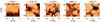 |
Fig. 17 Magnetic field configuration at the upper surface for DNS Runs a30/1–a30/3 of Table 5. |
| In the text | |
|
Fig. 18 Normalized spectra of Bz from DNS Run a30/4 at normalized times |
| In the text | |
|
Fig. 19 Normalized spectra of Bz from DNS Run A40/1 at normalized times |
| In the text | |
|
Fig. 20 Same as Fig. 13, but for the ILES runs with varying forcing amplitude. Note the different vertical extent of this set of models. The different lines indicate Ma = 0.16 (solid), 0.34 (dotted), and 0.68 (dashed). |
| In the text | |
|
Fig. 21 Same as Fig. 20, but for the ILES runs which vary both the forcing amplitude and the imposed magnetic field at the same time, keeping the relative field strength comparable. The different lines again indicate Ma = 0.16 (solid), 0.35 (dotted), and 0.68 (dashed), and agree markedly well in the lower panel where we plot relative to Beq(z). |
| In the text | |
|
Fig. 22 Surface appearance of the vertical magnetic field, |
| In the text | |
Current usage metrics show cumulative count of Article Views (full-text article views including HTML views, PDF and ePub downloads, according to the available data) and Abstracts Views on Vision4Press platform.
Data correspond to usage on the plateform after 2015. The current usage metrics is available 48-96 hours after online publication and is updated daily on week days.
Initial download of the metrics may take a while.