| Issue |
A&A
Volume 562, February 2014
|
|
|---|---|---|
| Article Number | A133 | |
| Number of page(s) | 17 | |
| Section | Planets and planetary systems | |
| DOI | https://doi.org/10.1051/0004-6361/201322342 | |
| Published online | 21 February 2014 | |
A non-grey analytical model for irradiated atmospheres⋆
I. Derivation
1
Laboratoire Lagrange, UMR7293, Université de Nice Sophia-Antipolis, CNRS,
Observatoire de la Côte d’Azur,
06300
Nice,
France
e-mail:
This email address is being protected from spambots. You need JavaScript enabled to view it.
2
Department of Astronomy and Astrophysics, University of
California, Santa
Cruz, CA
95064,
USA
Received:
22
July
2013
Accepted:
25
November
2013
Abstract
Context. Semi-grey atmospheric models (with one opacity for the visible and one opacity for the infrared) are useful for understanding the global structure of irradiated atmospheres, their dynamics, and the interior structure and evolution of planets, brown dwarfs, and stars. When compared to direct numerical radiative transfer calculations for irradiated exoplanets, however, these models systematically overestimate the temperatures at low optical depths, independently of the opacity parameters.
Aims. We investigate why semi-grey models fail at low optical depths and provide a more accurate approximation to the atmospheric structure by accounting for the variable opacity in the infrared.
Methods. Using the Eddington approximation, we derive an analytical model to account for lines and/or bands in the infrared. Four parameters (instead of two for the semi-grey models) are used: a visible opacity (κv), two infrared opacities, (κ1 and κ2), and β (the fraction of the energy in the beam with opacities κ1). We consider that the atmosphere receives an incident irradiation in the visible with an effective temperature Tirr and at an angle μ∗, and that it is heated from below with an effective temperature Tint.
Results. Our non-grey, irradiated line model is found to provide a range of temperatures that is consistent with that obtained by numerical calculations. We find that if the stellar flux is absorbed at optical depth larger than τlim = (κR/κ1κ2)(κRκP/3)1/2, it is mainly transported by the channel of lowest opacity whereas if it is absorbed at τ ≳ τlim it is mainly transported by the channel of highest opacity, independently of the spectral width of those channels. For low values of β (expected when lines are dominant), we find that the non-grey effects significantly cool the upper atmosphere. However, for β ≳ 1/2 (appropriate in the presence of bands with a wavelength-dependence smaller than or comparable to the width of the Planck function), we find that the temperature structure is affected down to infrared optical depths unity and deeper as a result of the so-called blanketing effect.
Conclusions. The expressions that we derive can be used to provide a proper functional form for algorithms that invert the atmospheric properties from spectral information. Because a full atmospheric structure can be calculated directly, these expressions should be useful for simulations of the dynamics of these atmospheres and of the thermal evolution of the planets. Finally, they should be used to test full radiative transfer models and to improve their convergence.
Key words: radiative transfer / planets and satellites: atmospheres / stars: atmospheres / planetary systems
A FORTRAN implementation of the analytical model is available at the CDS via anonymous ftp to cdsarc.u-strasbg.fr (130.79.128.5) or via http://cdsarc.u-strasbg.fr/viz-bin/qcat?J/A+A/562/A133
© ESO, 2014
1. Introduction
The discovery of numerous star-planet systems and the possibility of characterizing the planets’ atmospheric properties has led to a great many publications using radiative transfer calculations, often taken “off-the-shelf” from numerical models. Given the infinite amount of possible compositions for mostly unknown exoplanetary atmospheres, it is highly valuable to be able to perform very fast calculations and also to understand what determines the thermal structure of an irradiated atmosphere.
Analytical radiative transfer solutions for atmospheres have been calculated with a variety of assumptions and in different contexts (e.g. Eddington 1916; Chandrasekhar 1935, 1960; King 1956; Matsui & Abe 1986; Weaver & Ramanathan 1995; Pujol & North 2003; Chevallier et al. 2007; Shaviv et al. 2011). However, the discovery of super-Earths, giant exoplanets, brown dwarfs, and low-mass stars close to a source of intense radiation has prompted the need for solutions that account for both an outside and an inside radiation field, and properly link low and high optical depths levels. Hubeny et al. (2003), Rutily et al. (2008), Hansen (2008), Guillot (2010), Robinson & Catling (2012), and Heng et al. (2012) provide these solutions in the framework of a semi-grey model, with one opacity for the incoming irradiation (generally mostly at visible wavelengths), and one opacity for the thermal radiation field (generally mostly at infrared wavelengths). These approximations have been used in hydrodynamical models of planetary atmospheres (e.g. Heng et al. 2011; Rauscher & Menou 2013), planetary evolution models (e.g. Miller-Ricci & Fortney 2010; Guillot & Havel 2011; Budaj et al. 2012), planet synthesis models (Mordasini et al. 2012a,b), retrieval methods (Line et al. 2012), and a variety of other applications.
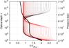 |
Fig. 1 Optical depth vs. atmospheric temperature in units of the effective temperature. A
numerical solution obtained from Fortney et al.
(2008) (thick black line) is compared to the semi-grey analytical solutions
of Guillot (2010) for values of the greenhouse
factor |


As shown in Fig. 1 for an atmosphere irradiated from
above with a flux  and heated from below
with a flux
and heated from below
with a flux  , while semi-grey
models provide solutions that are well-behaved when compared to full numerical solutions at
optical depths larger than about unity, the temperatures at low-optical depths appear to be
systematically hotter than in the numerical solutions. Most importantly, this occurs
regardless of the choice of the two parameters
of the problem, i.e. the thermal (infrared) opacity κth and the ratio
of the visible to infrared opacity γv ≡ κv/κth.
For hot Jupiters, as in the example in Fig. 1, the real
temperature profiles at low optical depths can be several hundreds of Kelvins cooler than
predicted by the semi-grey solutions.
, while semi-grey
models provide solutions that are well-behaved when compared to full numerical solutions at
optical depths larger than about unity, the temperatures at low-optical depths appear to be
systematically hotter than in the numerical solutions. Most importantly, this occurs
regardless of the choice of the two parameters
of the problem, i.e. the thermal (infrared) opacity κth and the ratio
of the visible to infrared opacity γv ≡ κv/κth.
For hot Jupiters, as in the example in Fig. 1, the real
temperature profiles at low optical depths can be several hundreds of Kelvins cooler than
predicted by the semi-grey solutions.
The levels probed both by transit spectroscopy and by the observations of secondary eclipses of exoplanets often correspond to low-optical depth levels (e.g. Burrows et al. 2007; Fortney et al. 2008; Showman et al. 2009), i.e. where semi-grey models seem to systematically overestimate the temperatures. Furthermore, because the problem persists regardless of the main parameters, this implies that the functional form of the semi-grey solutions is probably not appropriate for inversion models. Non-grey effects are known to facilitate the cooling of the upper atmosphere (see Pierrehumbert 2010, for a qualitative explanation) so they must be included. This is the purpose of the present paper.
We first describe previous analytical methods used to solve the radiative transfer problem analytically. In Sect. 3, we then derive an analytical non-grey line model and compare it to previous models in Sect. 4. In Sect. 5 we study the role of non-grey effects in shaping the atmospheric thermal structure. Eventually we apply our model to the structure of irradiated giant planets in Sect. 6. We note here that while we focus the discussion on exoplanets, we believe that this model is applicable to a much wider variety of problems, as long as an atmosphere is irradiated both from above and below. Our method can also be used to solve the radiative transfer equations in other geometries, such as the thermal structure of protoplanetary disk. We provide our conclusions in Sect. 7.
2. Assumptions and previous analytical models
2.1. Setting
2.1.1. The equation of radiative transfer
Following Guillot (2010), we will consider the
problem of a plane-parallel atmosphere in local thermodynamic equilibrium that receives
from above a collimated flux at an angle
θ∗ = cos-1(μ∗)
from the vertical, and from below an isotropic flux
. The total
energy budget of the modelled atmosphere is then set by
 , which defines
the effective temperature in this paper1.The
irradiation and intrinsic fluxes are generally characterized by very different
wavelengths. Although this is not required in the solution that we propose, it is
convenient to think of them as being emitted preferentially in the visible and in the
infrared, respectively. Scattering processes can influence both the thermal and visible
radiation. As shown by Heng et al. (2012), the
solution including symmetrical scattering for the incoming radiation with the Eddington
approximation is equivalent to the one obtained without scattering when the irradiation
flux is reduced by a factor of (1 − A) and the visible opacity is reduced by a
factor 1/
, which defines
the effective temperature in this paper1.The
irradiation and intrinsic fluxes are generally characterized by very different
wavelengths. Although this is not required in the solution that we propose, it is
convenient to think of them as being emitted preferentially in the visible and in the
infrared, respectively. Scattering processes can influence both the thermal and visible
radiation. As shown by Heng et al. (2012), the
solution including symmetrical scattering for the incoming radiation with the Eddington
approximation is equivalent to the one obtained without scattering when the irradiation
flux is reduced by a factor of (1 − A) and the visible opacity is reduced by a
factor 1/ ,
where A is the Bond albedo of the planet and ξ is the ratio of the absorption to the
extinction opacity (see also Meador & Weaver
1980, for a review of the different two stream methods including scattering).
In this paper, the irradiation flux and the visible opacity are treated as parameters,
thus we implicitly take into account symmetrical scattering of the incoming radiation
(e.g. Rayleigh scattering). Scattering of the thermal radiation, however, is neglected.
,
where A is the Bond albedo of the planet and ξ is the ratio of the absorption to the
extinction opacity (see also Meador & Weaver
1980, for a review of the different two stream methods including scattering).
In this paper, the irradiation flux and the visible opacity are treated as parameters,
thus we implicitly take into account symmetrical scattering of the incoming radiation
(e.g. Rayleigh scattering). Scattering of the thermal radiation, however, is neglected.
In order to solve the radiative transfer problem for a plane parallel atmosphere in
local thermodynamic equilibrium, one has to solve the following equation for all
frequencies ν and all directions μ (Chandrasekhar 1960), 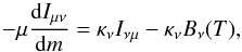 (1)where Iμν is the specific
intensity at the wavelength ν propagating with an angle θ = cos-1(μ) with the
vertical, κν is the opacity
at a given wavelength, Bν is the Planck
function, and dm = ρdz is the
mass increment along the path of the radiation. As usual, T, ρ, and z are the atmospheric
temperature, density and height, respectively. The main difficulty in solving Eq. (1)lies in its triple dependence on
μ,
ν, and
T and its
additional dependence on m. An analytical solution requires simplifications
of the opacities and of the dependence of the radiation intensity on angle.
(1)where Iμν is the specific
intensity at the wavelength ν propagating with an angle θ = cos-1(μ) with the
vertical, κν is the opacity
at a given wavelength, Bν is the Planck
function, and dm = ρdz is the
mass increment along the path of the radiation. As usual, T, ρ, and z are the atmospheric
temperature, density and height, respectively. The main difficulty in solving Eq. (1)lies in its triple dependence on
μ,
ν, and
T and its
additional dependence on m. An analytical solution requires simplifications
of the opacities and of the dependence of the radiation intensity on angle.
2.1.2. Opacities and optical depth
The need for simplification implies that mean opacities must be used. The most common
one is the Rosseland mean, defined as 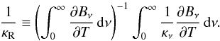 (2)When at all wavelengths
the mean free path of photons is small compared to the scale height of the atmosphere,
the radiative gradient obeys its well-defined diffusion limit and (unless convection
sets in) the temperature gradient become that obtained from a grey atmosphere in which
the opacity is set to the Rosseland mean (Mihalas
& Mihalas 1984, p. 350). We hence define the optical depth
τ on the
basis of the Rosseland mean opacity, such that, along the vertical direction
(2)When at all wavelengths
the mean free path of photons is small compared to the scale height of the atmosphere,
the radiative gradient obeys its well-defined diffusion limit and (unless convection
sets in) the temperature gradient become that obtained from a grey atmosphere in which
the opacity is set to the Rosseland mean (Mihalas
& Mihalas 1984, p. 350). We hence define the optical depth
τ on the
basis of the Rosseland mean opacity, such that, along the vertical direction
 (3)Assuming
hydrostatic equilibrium, the relation between pressure and optical depth can be found by
integrating Eq. (3):
(3)Assuming
hydrostatic equilibrium, the relation between pressure and optical depth can be found by
integrating Eq. (3):  (4)The optical
depth thus becomes the natural variable to account for the dependence on depth in the
radiative transfer problem. For any strictly positive Rosseland mean opacities, Eq.
(4)is a bijection relating pressure and
optical depth. Thus, solution of the radiative transfer equations in terms of optical
depth can be converted to a solution in term of pressure for any functional form of the
Rosseland mean opacities.
(4)The optical
depth thus becomes the natural variable to account for the dependence on depth in the
radiative transfer problem. For any strictly positive Rosseland mean opacities, Eq.
(4)is a bijection relating pressure and
optical depth. Thus, solution of the radiative transfer equations in terms of optical
depth can be converted to a solution in term of pressure for any functional form of the
Rosseland mean opacities.
The second mean opacity that is traditionally used for radiative transfer is the
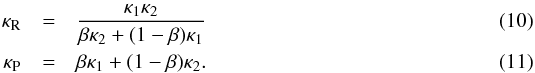
so-called Planck mean:  (5)We use the
ratio of the Planck and Rosseland mean opacities to quantify the non-greyness of the
atmosphere:
(5)We use the
ratio of the Planck and Rosseland mean opacities to quantify the non-greyness of the
atmosphere:  (6)While
the value of the Rosseland mean opacity is dominated by the lowest values of the opacity
function κν, the Planck mean
opacity is dominated by its highest values. Thus, it can be shown that γP = 1 for a
grey atmosphere and γP > 1 for a
non-grey atmosphere (King 1956).
(6)While
the value of the Rosseland mean opacity is dominated by the lowest values of the opacity
function κν, the Planck mean
opacity is dominated by its highest values. Thus, it can be shown that γP = 1 for a
grey atmosphere and γP > 1 for a
non-grey atmosphere (King 1956).
In irradiated atmospheres, a collimated flux coming from the star is absorbed at different atmospheric levels. We name κv the opacity relevant to the absorption of the stellar flux. As will be shown in Sect. 3.8, the absorption of the visible flux appears linearly in the radiative transfer equations. Thus, a solution can be found using multiple visible opacity bands κv1, κv2, etc.
We further define the ratio of the visible opacity to the mean (Rosseland) thermal
opacity:  (7)In order to solve the
radiative transfer problem analytically, we suppose that γv is constant
with optical depth. Once γv is chosen, we can solve the
equations for the visible radiation independently from the final thermal structure of
the atmosphere. Of course, purely grey models are such that γv = 1.
(7)In order to solve the
radiative transfer problem analytically, we suppose that γv is constant
with optical depth. Once γv is chosen, we can solve the
equations for the visible radiation independently from the final thermal structure of
the atmosphere. Of course, purely grey models are such that γv = 1.
2.1.3. The picket-fence model
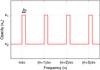 |
Fig. 2 Simplified thermal opacities for the picket-fence model. β = δν/Δν is the equivalent bandwidth (see text). |
It is important to note at this point that two sets of opacities with different
wavelength dependences may have the same Rosseland and Planck means. We
must constrain the problem further, and to this intent, we now consider the simplest
possible line model, known as the picket-fence model (Mihalas 1978), where the thermal opacities can take two different values
κ1 and κ2 (see Fig.
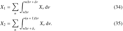
2) such that ![Mathematical equation: \begin{equation} \Knu= \left\{ \begin{array}{l l} \Ka & \quad \mbox{for }\nu\in[n\Delta\nu,n\Delta\nu+\delta\nu]\\ \Kb & \quad \mbox{for }\nu\in[n\Delta\nu+\delta\nu,(n+1)\Delta\nu]\\ \end{array} \right. \hspace{0.3cm} n\in[1,N] . \label{eq::CombOpacities} \end{equation}](/articles/aa/full_html/2014/02/aa22342-13/aa22342-13-eq58.png) (8)We define an equivalent
bandwidth by:
(8)We define an equivalent
bandwidth by: 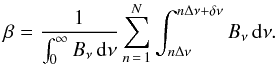 (9)The
characteristic width of the Planck function can be defined as
(9)The
characteristic width of the Planck function can be defined as
 .
When choosing Δν ≪ ΔνP,
the Planck function can be considered constant over Δν and we get
β = δν/Δν. The Planck and
Rosseland mean opacities then become (see Eqs. (2)and (5))
.
When choosing Δν ≪ ΔνP,
the Planck function can be considered constant over Δν and we get
β = δν/Δν. The Planck and
Rosseland mean opacities then become (see Eqs. (2)and (5))
 We
also define the following ratios:
We
also define the following ratios:  Following
Chandrasekhar (1935), we also define a limit
optical depth
Following
Chandrasekhar (1935), we also define a limit
optical depth  (15)The
role of τlim in shaping the final temperature
profile is discussed in Sect. 5 and its variations with
R and
β is
pictured in Fig. 8.
(15)The
role of τlim in shaping the final temperature
profile is discussed in Sect. 5 and its variations with
R and
β is
pictured in Fig. 8.
2.2. The method of discrete ordinates for the non-irradiated problem
2.2.1. The grey case
An approximate method to solve Eq. (1)
including the angular dependency has been developed by Chandrasekhar (1960) in the case of a non-irradiated atmosphere
(Tirr = 0). The idea is to replace the
integrals over angle in Eq. (1) by a
Gaussian sum over μ. It can then be solved to an arbitrary precision
by increasing the number of terms in the sum. The boundary condition at the top of the
atmosphere is simply given as Iμ < 0(0) = 0.
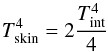
The expansion to the fourth term yields the temperature profile
 (16)with
Q = 0.706920, L1 = −0.083921, L2 = −0.036187, L3 = −0.009461, k1 = 1.103188,
k2 = 1.591778, and k3 = 4.45808
(Chandrasekhar 1960, Table VIII)2. One of the important results from this formalism is
that the skin temperature of the planet (defined as the temperature at zero optical
depth) is independent of the order of expansion and therefore corresponds to the exact
value
(16)with
Q = 0.706920, L1 = −0.083921, L2 = −0.036187, L3 = −0.009461, k1 = 1.103188,
k2 = 1.591778, and k3 = 4.45808
(Chandrasekhar 1960, Table VIII)2. One of the important results from this formalism is
that the skin temperature of the planet (defined as the temperature at zero optical
depth) is independent of the order of expansion and therefore corresponds to the exact
value  (17)This
expression is exact only in the limit of a grey, non-irradiated atmosphere.
(17)This
expression is exact only in the limit of a grey, non-irradiated atmosphere.
2.2.2. The non-grey case
Chandrasekhar (1960) also developed a
perturbation method in order to include non-grey thermal opacities. This method was
improved by Krook (1963). However, these
perturbation methods either work for small departures from the grey opacities or involve
a fastidious iterative procedure (e.g. Unno &
Yamashita 1960; Avrett & Krook
1963) and are no longer fully analytical. However, considering that the
variations in the opacities are small compared to the variations of the Planck function,
analytical solutions can be found for an arbitrarily large departure from the grey
opacities. Noting the similar role of μ and κν in Eq. (1), King
(1956), following Münch (1946), used the
method of discrete ordinates in order to turn the integrals over frequency into Gaussian
sums. For the picket-fence model defined in Sect. 2.1.3 and the second approximation for the angular dependency, King’s method
leads to the following temperature profile ![Mathematical equation: \begin{equation} T^{4}(\tau)\!=\!\frac{3}{4}\tint^{4}\left[\frac{1}{\sqrt{3\Gp}}\!+\!\tau+\frac{(\sqrt{\Gp}-\Ga)(\sqrt{\Gp}-\Gb)}{\Ga\Gb\sqrt{3\Gp}}({\rm e}^{-\tau/\taulim}-1)\right]\cdot \label{eq::T4King} \end{equation}](/articles/aa/full_html/2014/02/aa22342-13/aa22342-13-eq78.png) (18)As
in the grey case, the method of discrete ordinates leads to an exact relation for the
skin temperature, whatever the dependency of κν on frequency (but
no dependence on pressure or temperature):
(18)As
in the grey case, the method of discrete ordinates leads to an exact relation for the
skin temperature, whatever the dependency of κν on frequency (but
no dependence on pressure or temperature):  (19)In
the grey limit, γP = 1 and we recover Eq. (17). Otherwise, γP > 1, implying
that for a non-irradiated atmosphere, non-grey effects always tend to lower the
atmospheric skin temperature.
(19)In
the grey limit, γP = 1 and we recover Eq. (17). Otherwise, γP > 1, implying
that for a non-irradiated atmosphere, non-grey effects always tend to lower the
atmospheric skin temperature.
2.3. Moment equation method
2.3.1. Equations for the momentum of the radiation intensity
A simpler way to solve the radiative transfer equation has been carried out by Eddington (1916). The idea is to solve the equation
using the different momentum of the intensity defined as  (20)Then, integrating
over μ Eq.
(1)and μ times Eq. (1)one gets the momentum equations
(20)Then, integrating
over μ Eq.
(1)and μ times Eq. (1)one gets the momentum equations
 Assuming
the atmosphere to be in radiative equilibrium, we can write
Assuming
the atmosphere to be in radiative equilibrium, we can write  (23)For a grey atmosphere
(κν = κR ∀ν),
Eqs. (21)−(23) can be integrated over frequency, leading to an equation for
J,
H,
K, and
B, the
frequency-integrated versions of Jν, Hν, Kν, and Bν. The radiative
equilibrium equation becomes
(23)For a grey atmosphere
(κν = κR ∀ν),
Eqs. (21)−(23) can be integrated over frequency, leading to an equation for
J,
H,
K, and
B, the
frequency-integrated versions of Jν, Hν, Kν, and Bν. The radiative
equilibrium equation becomes  (24)The frequency
integrated versions of Eqs. (21)−(23) are a set of three equations with four
unknowns. The system is not closed because by integrating Eq. (1) over all angles we have lost the
information on the angular dependency of the irradiation. A closure relationship that
contains this angular dependency is therefore needed. A common closure relationship,
known as the Eddington approximation is
(24)The frequency
integrated versions of Eqs. (21)−(23) are a set of three equations with four
unknowns. The system is not closed because by integrating Eq. (1) over all angles we have lost the
information on the angular dependency of the irradiation. A closure relationship that
contains this angular dependency is therefore needed. A common closure relationship,
known as the Eddington approximation is
 (25)This
relationship is exact in two very different cases: when the radiation field is isotropic
(Iμ independent of
μ), and
in the two-stream approximation (
(25)This
relationship is exact in two very different cases: when the radiation field is isotropic
(Iμ independent of
μ), and
in the two-stream approximation ( and
and
 ). Although
this seems to be a very restrictive approximation, it is relevant for the deep layers of
the atmosphere because of the quasi-isotropy of the radiation field there. It is also
good for the top of the atmosphere, where the flux comes mainly from the τ ≈ 1 layer. Indeed, the
exact solution gives a ratio J/K that differs by no more than 20% from the 1/3 ratio over the
whole atmosphere and leads to a temperature profile that is correct to 4% in the grey case (see the plain blue
line in Fig. 4).
). Although
this seems to be a very restrictive approximation, it is relevant for the deep layers of
the atmosphere because of the quasi-isotropy of the radiation field there. It is also
good for the top of the atmosphere, where the flux comes mainly from the τ ≈ 1 layer. Indeed, the
exact solution gives a ratio J/K that differs by no more than 20% from the 1/3 ratio over the
whole atmosphere and leads to a temperature profile that is correct to 4% in the grey case (see the plain blue
line in Fig. 4).
2.3.2. Top boundary condition
Although in the method of discrete ordinates the boundary condition at the top of the atmosphere is intuitive, in the momentum equations method it is less obvious and different choices have been made by different authors. Usually, the expression for J is known and some integration constants need to be found. Two equations are needed, one for J(0) and one for H(0). Four possibilities are widely used in the literature from which one has to choose two:
-
1.
The radiative equilibrium equation that relates the emergent flux at the top of the atmosphere to the internal flux from the planet and the incident flux from the star.
-
2.
An ad-hoc relation between H(0) and J(0) at τ = 0: H(0) = fHJ(0), where fH is often called the second Eddington coefficient.
-
3.
A calculation of H(0) from the second moment equation (Eq. (22)) and the Eddington approximation.
-
4.
A calculation of H(0) from the integration of the source function through the entire atmosphere, known as the Milne equation (Mihalas & Mihalas 1984, p. 347):
 .
.
For grey and semi-grey models, the first condition is natural and so it was used by Hansen (2008) and Guillot (2010). For the other part of the top boundary condition, Guillot (2010) chose to use the second and Hansen (2008) the fourth condition (see Appendix A of Guillot 2010 for a comparison of the two expressions).
In the case of a non-grey model, the first condition cannot be implemented (at least directly) because it is a constraint on the total thermal flux, but it provides no information on how the thermal flux is split between the opacity bands that are considered. Chandrasekhar (1935) therefore uses conditions 2 and 3 in each of the opacity bands for his non-grey, non-irradiated model. He also notes that using condition 4 instead of condition 3 should yield better results, but it leads to more complex expressions. In this work, because an accurate treatment of the flux is needed for the non-grey irradiated model, we will use conditions 2 and 4 in each of the opacity bands. All these models are discussed in the next sections and summarized in Table 1.
2.3.3. Non-irradiated, grey case
In this section we consider the case Tirr = 0. Under the grey
approximation, using the conditions 1 and 4, the temperature profile is given by (Mihalas & Mihalas 1984, p. 357)
 (26)which leads to
the same solution as assuming condition 2 with
(26)which leads to
the same solution as assuming condition 2 with  . The skin temperature is then
 (27)which
differs from the exact solution (Eq. (17)) by a factor of
(27)which
differs from the exact solution (Eq. (17)) by a factor of  /2. Assuming
 /
/ is thus tempting, as it leads to the correct skin temperature. Unfortunately, it leads
to a temperature profile which is less accurate around τ ≈ 1.
is thus tempting, as it leads to the correct skin temperature. Unfortunately, it leads
to a temperature profile which is less accurate around τ ≈ 1.
2.3.4. Non-irradiated non-grey picket-fence model
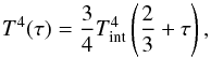
Chandrasekhar (1935) provides solutions to the
moment equations for the picket-fence model presented in Sect. 2.1.3. He assumes that the relation
 with
,
valid in the grey case under the Eddington approximation (see Eq. (27)), holds for the two thermal channels
separately. Using this condition together with condition 3, he obtains a temperature
profile
with
,
valid in the grey case under the Eddington approximation (see Eq. (27)), holds for the two thermal channels
separately. Using this condition together with condition 3, he obtains a temperature
profile ![Mathematical equation: \begin{eqnarray} \label{eq::T4Chandra} T^{4}(\tau)&=&\frac{3\tint^{4}}{4}\left[\tau+\frac{\frac{2}{3}+\sqrt{\frac{1}{3\Gp}}}{1+\frac{1}{2}\sqrt{3\Gp}}\right]\nonumber\\ &&\hspace*{4mm}+\frac{3\tint^{4}}{4}\left(\frac{\Gp-1}{\sqrt{\Gp}}\right)\frac{\frac{1}{\sqrt{3}}+\sqrt{\Gp}\taulim}{1+\frac{1}{2}\sqrt{3\Gp}}\left(1-{\rm e}^{-\tau/\taulim}\right) \end{eqnarray}](/articles/aa/full_html/2014/02/aa22342-13/aa22342-13-eq116.png) (28)and
an equation for the skin temperature
(28)and
an equation for the skin temperature 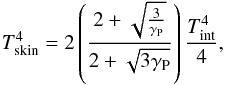 (29)As expected, this
equation reduces to Eq. (27) in the
limit γP = 1. For high values of
γP, this relation differs by a factor of
4/3
from the exact one derived with the method of discrete ordinates [19]. As happens for the grey case, using
/
would lead to the exact solution for the skin temperature, but at the expense of the
accuracy of the profile at deeper levels. Again, we note that, in the non-irradiated
case, the temperature at the top of the atmosphere is determined by a single parameter,
γP, representing the non-greyness of the
atmosphere. A comparison of the different expressions for the skin temperature is
provided in Sect. 4.
(29)As expected, this
equation reduces to Eq. (27) in the
limit γP = 1. For high values of
γP, this relation differs by a factor of
4/3
from the exact one derived with the method of discrete ordinates [19]. As happens for the grey case, using
/
would lead to the exact solution for the skin temperature, but at the expense of the
accuracy of the profile at deeper levels. Again, we note that, in the non-irradiated
case, the temperature at the top of the atmosphere is determined by a single parameter,
γP, representing the non-greyness of the
atmosphere. A comparison of the different expressions for the skin temperature is
provided in Sect. 4.
2.3.5. Irradiated semi-grey model
In the case of irradiated atmospheres, the presence of an incoming collimated flux at the top of the atmosphere breaks the angular symmetry of the equations. The radiative transfer problem thus can no longer be solved analytically (at least not in a simple way) through the discrete ordinates technique. The momentum method is thus required.
To solve the problem, the radiation field is split into two parts: the incoming, collimated radiation field on one hand, the thermal radiation field on the other. The radiative equilibrium equation (Eq. (23)) links the two streams, as can be seen in Sect. 3.1 (see also Hansen 2008; Guillot 2010; Robinson & Catling 2012). As mentioned in Sect. 2.1.2, when the incident radiation is at a much shorter wavelength than the thermal emission of the atmosphere, the two streams correspond to different characteristic wavelengths and may often be labelled as visible and infrared. This is not a requirement, however: the solutions apply if the radiation field corresponds to other wavelengths or if they overlap.
As discussed previously (Sect. 2.3.2), the
boundary condition at the top of the model can be chosen in several ways. When using
condition 2, Guillot (2010) lets the value of
 be either
1/2 or
be either
1/2 or
 .
Those values are based on the non-irradiated case:
is
the value that arises from the calculation of the angle dependence between
H(0) and
J(0) in
the isotropic case, but
.
Those values are based on the non-irradiated case:
is
the value that arises from the calculation of the angle dependence between
H(0) and
J(0) in
the isotropic case, but  provides a skin temperature that agrees with the exact value. The two solutions differ
by ≈3% at most (see Fig.
5 hereafter), and choosing one over another is
not crucial. In any case, for an easier comparison, we provide here the solution of
Guillot (2010) for
provides a skin temperature that agrees with the exact value. The two solutions differ
by ≈3% at most (see Fig.
5 hereafter), and choosing one over another is
not crucial. In any case, for an easier comparison, we provide here the solution of
Guillot (2010) for
![Mathematical equation: \begin{eqnarray} \label{eq::T4Guillot} T^4&=&{3\tint^4\over 4}\left[{2\over 3}+\tau\right]\nonumber\\ &&+{3\tirr^4\over 4}\mu_*\left[{2\over 3}+ {\mu_*\over \Gv}+\left({\Gv\over 3\mu_*}-{\mu_*\over\Gv}\right) {\rm e}^{-\Gv\tau/\mu_*}\right], \end{eqnarray}](/articles/aa/full_html/2014/02/aa22342-13/aa22342-13-eq125.png) (30)where
μ∗ is the cosine of the angle of the
incident radiation. The skin temperature is
(30)where
μ∗ is the cosine of the angle of the
incident radiation. The skin temperature is  (31)For γv → 0, the
incident radiation is absorbed in the deep layers of the atmosphere and the skin
temperature converges to the skin temperature of a grey model with an effective
temperature
(31)For γv → 0, the
incident radiation is absorbed in the deep layers of the atmosphere and the skin
temperature converges to the skin temperature of a grey model with an effective
temperature  . The semi-grey
model depends only on the parameter γv.
. The semi-grey
model depends only on the parameter γv.
As discussed in the introduction, the semi-grey model predicts minimum temperatures that are generally higher than the numerical solutions for irradiated exoplanets, independent of the choice of γv (see Fig. 1). In fact, similarly to the skin temperature, the minimum temperature of a semi-grey atmosphere, shown in Fig. 3, depends only on the values of Teff, μ∗ and γv. It is the lowest and equal to Teff, μ∗/21/4 both in the γv → 0 and γv → ∞ limits. This lower bound for the semi-grey temperature profile is hotter than the one obtained by numerical calculations taking into account the full set of opacities. The discrepancy is much larger than the variations resulting from the approximation of the momentum method. Clearly, non-grey effects must be invoked to explain the low temperatures obtained by numerical models at low optical depths.
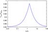 |
Fig. 3 Minimum temperature of the semi-grey model in terms of the effective temperature as a function of γv/μ∗. |
Summary of the different models compared in this paper.
3. An analytical irradiated non-grey picket-fence model
3.1. Equations
We now derive the equations for an irradiated atmosphere in local thermodynamic equilibrium with infrared line opacities as described in Sect. 2.1.2. Thus, our model contains three different opacities: κ1 and κ2 for the thermal radiation and κv for the incoming radiation of the star. As explained before, the difference between the thermal and the visible channel depends on the angular dependency of the radiation and not on the frequency. Although the method of discrete ordinates is shown to lead to more exact results, it is difficult to adapt to the irradiated case. Therefore, following Chandrasekhar (1935) and Guillot (2010), we solve the radiative transfer equations using the momentum equations. Integrating Eqs. (21) and (22) over each thermal band we obtain
 where
the subscript indicates the integrated quantities over the given thermal band. Thus, for a
quantity Xν we have:
where
the subscript indicates the integrated quantities over the given thermal band. Thus, for a
quantity Xν we have:
 The
Planck function is considered constant over each bin of frequency Δν and therefore
B1 = βB and
B2 = (1 − β)B.
The
Planck function is considered constant over each bin of frequency Δν and therefore
B1 = βB and
B2 = (1 − β)B.
We now assume that the Eddington approximation is valid in the two bands separately:
J(1,2) = 3K(1,2).
Equations (32)and (33)can be combined into 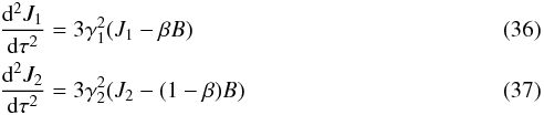 and
the radiative equilibrium equation becomes
and
the radiative equilibrium equation becomes  (38)where the quantities
with subscript v are the
momentum of the incident stellar radiation. Assuming that the incoming stellar radiation
arrives as a collimated flux and hit the top of the atmosphere with an angle
θ∗ = cos-1μ∗
they can are given by
(38)where the quantities
with subscript v are the
momentum of the incident stellar radiation. Assuming that the incoming stellar radiation
arrives as a collimated flux and hit the top of the atmosphere with an angle
θ∗ = cos-1μ∗
they can are given by  (39)with
 the total incident intensity.
The absorption of the stellar irradiation can be treated separately from the thermal
radiation and Jv is given by Eq. (13) of Guillot (2010), 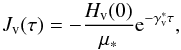 (40)where we have
simplified the notation by introducing the parameter
(40)where we have
simplified the notation by introducing the parameter
 .
.
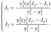
Equations (36) to (38) are a set of three coupled equations with
three unknowns J1, J2, and
B. In order
to decouple these equations we define two new variables:
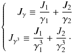 (41)Conversely,
we can come back to the original variables:
(41)Conversely,
we can come back to the original variables:
 (42)Using
the combination of Eqs.
(42)Using
the combination of Eqs.  (36) +
  (37) and (38)we get
 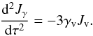 (43)The combination of
Eqs.
(43)The combination of
Eqs.  (36)+
(36)+ (37) yields
  (44)Noting that
 , Eq.
(38) becomes
, Eq.
(38) becomes  (45)Equations (43)−(45) are now a set of
two uncoupled differential equations and a linear equation.
(45)Equations (43)−(45) are now a set of
two uncoupled differential equations and a linear equation.
3.2. Boundary conditions
To solve the differential equations we need to specify the boundary conditions. When
τ → + ∞ we
want to fulfill the diffusion approximation Jν = Bν
(Mihalas & Mihalas 1984, p. 350). In our
case this translates to J1 = βB and
J2 = (1 − β)B.
Furthermore, at these levels, the gradient of B should also obey the diffusion
approximation (Mihalas & Mihalas 1984)
 (46)where
 is the
thermal flux coming from the interior of the planet. Using the system of Eqs. (41) and noting that
is the
thermal flux coming from the interior of the planet. Using the system of Eqs. (41) and noting that  , we can derive a condition on
Jγ and Jγ3:
, we can derive a condition on
Jγ and Jγ3:
 For
τ → 0 we
specify the geometry of the intensity by setting:
For
τ → 0 we
specify the geometry of the intensity by setting:  (49)Furthermore, we
calculate the flux at the top of the atmosphere in each band using Eq. (79.21) from Mihalas & Mihalas (1984). From the assumption
of local thermodynamic equilibrium, the source function in the two bands is
S1(τ1) = βB(τ/γ1)
and S2(τ2) = (1 − β)B(τ/γ2).
The upper boundary condition on the flux of the two bands thus becomes
(49)Furthermore, we
calculate the flux at the top of the atmosphere in each band using Eq. (79.21) from Mihalas & Mihalas (1984). From the assumption
of local thermodynamic equilibrium, the source function in the two bands is
S1(τ1) = βB(τ/γ1)
and S2(τ2) = (1 − β)B(τ/γ2).
The upper boundary condition on the flux of the two bands thus becomes  (50)
(50)
3.3. Solution
The solution of a second-order differential equation with constant coefficient is the sum
of the solutions of the homogeneous equation and a particular solution of the complete
equation. Thus, solutions of Eq. (43) must
be of the form:  (51)Applying the
boundary condition Eq. (47), we get
C2 = 3H. For
τ = 0 we
obtain
(51)Applying the
boundary condition Eq. (47), we get
C2 = 3H. For
τ = 0 we
obtain  (52)Using Eq. (45)to eliminate B and replacing
Jγ by its solution, Eq.
(44) becomes:
(52)Using Eq. (45)to eliminate B and replacing
Jγ by its solution, Eq.
(44) becomes:  (53)Again,
solutions of this differential equation must be the sum of the solutions of the
homogeneous equation and one solution of the complete equation. The homogeneous solution
must have the form
(53)Again,
solutions of this differential equation must be the sum of the solutions of the
homogeneous equation and one solution of the complete equation. The homogeneous solution
must have the form  (54)where
C3 and C4 are constants
of integration to be determined using the boundary conditions. We look for a particular
solution formed by the superposition of an exponential and an affine function. The affine
function must then be a solution of Eq. (53) with Hv(0) = 0
(54)where
C3 and C4 are constants
of integration to be determined using the boundary conditions. We look for a particular
solution formed by the superposition of an exponential and an affine function. The affine
function must then be a solution of Eq. (53) with Hv(0) = 0 (55)and the exponential
function must be solution of Eq. (53),
keeping only the exponential part on the right-hand side
(55)and the exponential
function must be solution of Eq. (53),
keeping only the exponential part on the right-hand side
![Mathematical equation: \begin{equation} J_{\rm \gamma^{3} P2}\!=\!\frac{\Gp}{(\Ga\Gb)^{2}}\frac{1}{(\Gv^*\tau_{\rm lim})^{2}-1}\left[\left(1-\frac{\Ga^{2}\!+\!\Gb^{2}}{\Gp}\right)\frac{3}{\Gv^*}+\frac{\Gv^*}{\Gp}\right]\Hv(0){\rm e}^{-\Gv^*\tau} . \end{equation}](/articles/aa/full_html/2014/02/aa22342-13/aa22342-13-eq192.png) (56)Applying the
boundary condition defined by Eq. (48) to
the full solution Jγ3 = Jγ3P1 + Jγ3P2 + Jγ3H,
we find C4 = 0. The full solution of Eq. (44)is therefore given by
(56)Applying the
boundary condition defined by Eq. (48) to
the full solution Jγ3 = Jγ3P1 + Jγ3P2 + Jγ3H,
we find C4 = 0. The full solution of Eq. (44)is therefore given by  (57)We can get an
expression for the source function by replacing Jγ and Jγ3 in the
radiative equilibrium equation (Eq. (45)):
(57)We can get an
expression for the source function by replacing Jγ and Jγ3 in the
radiative equilibrium equation (Eq. (45)):
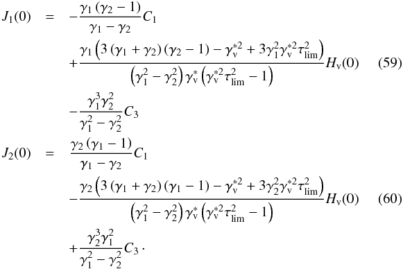
![Mathematical equation: \begin{eqnarray} \label{eq::BwithCste} B&=&\Ca+3H\tau-\frac{(\Ga\Gb)^{2}}{\Gp}\Cc {\rm e}^{-\tau/\tau_{\rm lim}}\nonumber\\ && \hspace*{4mm}+ \frac{\left[3-(\Gv^*/\Ga)^{2}\right]\left[3-(\Gv^*/\Gb)^{2}\right]}{3\Gv^*(1-\Gv^{*2}\taulim^{2})}\Hv(0){\rm e}^{-\Gv^*\tau}. \end{eqnarray}](/articles/aa/full_html/2014/02/aa22342-13/aa22342-13-eq196.png) (58)To
get the complete solution of the problem, we need to determine the two remaining
integration constants C1 and C3 using the
boundary condition (49). For that we need
to calculate J1(0), J2(0),
H1(0) and H2(0). The first
two quantities can be evaluated by inserting the values of Jγ(0) and Jγ3(0) from
Eqs. (51) and (57) into system (42):
(58)To
get the complete solution of the problem, we need to determine the two remaining
integration constants C1 and C3 using the
boundary condition (49). For that we need
to calculate J1(0), J2(0),
H1(0) and H2(0). The first
two quantities can be evaluated by inserting the values of Jγ(0) and Jγ3(0) from
Eqs. (51) and (57) into system (42):
 Noting
that
Noting
that
 we
can evaluate H1(0) and H2(0) by
inserting Eqs. (58) into (50). Then, Eq. (49) is a linear system of two equations with two unknowns. After some
calculations we get the expressions for C1 and C3
we
can evaluate H1(0) and H2(0) by
inserting Eqs. (58) into (50). Then, Eq. (49) is a linear system of two equations with two unknowns. After some
calculations we get the expressions for C1 and C3 where
we have
where
we have
![Mathematical equation: \begin{eqnarray} \label{eq::a0} a_0&=& {1\over \gamma_1}+{1\over \gamma_2} \\ \label{eq::a1} a_1&=&-{1\over 3\tau_{\rm lim}^2}\left[{\gamma_{\rm p}\over 1\!-\!\gamma_{\rm p}}{\gamma_1\!+\!\gamma_2-2\over \gamma_1+\gamma_2}+(\gamma_1+\gamma_2)\tau_{\rm lim}\!-\!(A_{\rm t,1}\!+\!A_{\rm t,2})\tau_{\rm lim}^2\right] \quad\quad\quad\\ a_{2} &=&\frac{\taulim^{2}}{\Gp\Gv^{*2}}\notag \\ \times&&\frac{\left(3\Ga^{2}\!-\!\Gv^{*2}\right)\left(3\Gb^{2}\!-\!\Gv^{*2}\right)\left(\Ga\!+\!\Gb\right)\!-\!3\Gv^*\left(6\Ga^{2}\Gb^{2}\!-\!\Gv^{*2}\left(\Ga^{2}\!+\!\Gb^{2}\right)\right)}{1\!-\!\Gv^{*2}\taulim^{2}} \quad\quad\quad\\ a_{3} &=&-\frac{\taulim^{2}(3\Ga^{2}-\Gv^{*2})(3\Gb^{2}-\Gv^{*2})(A_{\rm{v,2}}+A_{\rm v,1})}{\Gp\Gv^{*3}(1-\Gv^{*2}\taulim^{2})} \\ b_{0} &=&\left(\frac{\Ga\Gb}{\Ga\!-\!\Gb}\frac{A_{\rm t,1}\!-\!A_{\rm t,2}}{3}\!-\!\frac{(\Ga\Gb)^{2}}{\sqrt{3\Gp}}\!-\!\frac{(\Ga\Gb)^{3}}{(1-\Ga)(1-\Gb)(\Ga\!+\!\Gb)}\right)^{-1} \quad\quad\quad\\ b_{1} &=&\frac{\Ga\Gb(3\Ga^{2}-\Gv^{*2})(3\Gb^{2}-\Gv^{*2})\taulim^{2}}{\Gp\Gv^{*2}(\Gv^{*2}\taulim^{2}-1)} \\ b_{2} &=&\frac{3(\Ga+\Gb)\Gv^{*3}}{(3\Ga^{2}-\Gv^{*2})(3\Gb^{2}-\Gv^{*2})} \\ b_{3} &=&\frac{A_{\rm v,2}-A_{\rm v,1}}{\Gv^* (\Ga-\Gb)} , \end{eqnarray}](/articles/aa/full_html/2014/02/aa22342-13/aa22342-13-eq207.png) where
we defined
where
we defined 
3.4. Atmospheric temperature profile
Using the relations B = σT4/π,
 , and
, and
 and Eq. (58), we can derive the equation for the
temperature at any optical depth
and Eq. (58), we can derive the equation for the
temperature at any optical depth  (76)with
![Mathematical equation: \begin{eqnarray} \label{eq::A} &&A= {1\over3}(a_0+a_1b_0)\\ \label{eq::B} &&B= -{1\over3}{(\gamma_1\gamma_2)^2\over \gamma_{\rm p}}b_0\\ \label{eq::C} &&C=-{1\over3}\left[b_0 b_1 (1+b_2+b_3)a_1+a_2+a_3\right]\\ &&D={1\over3}{(\gamma_1\gamma_2)^2\over \gamma_{\rm p}}b_0 b_1(1+b_2+b_3)\\ &&E=\frac{\left[3-(\Gv^*/\Ga)^{2}\right]\left[3-(\Gv^*/\Gb)^{2}\right]}{9\Gv^*\left[(\Gv^*\taulim)^{2}-1\right]}\cdot \label{eq::E} \end{eqnarray}](/articles/aa/full_html/2014/02/aa22342-13/aa22342-13-eq213.png)
3.5. Grey limit
In the grey limit, γP → 1 (as γ1 and
γ
2
) and we obtain
 If
we also assume that
If
we also assume that  we
obtain
we
obtain  and
E → −1/
and
E → −1/ and the
solution converges towards that of Guillot (2010)
(see Eq. (30)). For other values of
our model
differs from the solutions of Guillot (2010, see also Hansen
2008) because of the different boundary conditions used in the two models (see
Sect. 2.3.2). However, calculations show that the
value of C
obtained here differs from the same coefficient extracted from Eq. (30) by at most 12% and that the two solutions
also converge for
and the
solution converges towards that of Guillot (2010)
(see Eq. (30)). For other values of
our model
differs from the solutions of Guillot (2010, see also Hansen
2008) because of the different boundary conditions used in the two models (see
Sect. 2.3.2). However, calculations show that the
value of C
obtained here differs from the same coefficient extracted from Eq. (30) by at most 12% and that the two solutions
also converge for  . As
seen in Fig. 5, in the semi-grey limit, and when
calculating the full temperature profile, our model differs by at most 2% from the Guillot (2010) model. The difference between the various solutions must be
attributed to the Eddington approximation.
. As
seen in Fig. 5, in the semi-grey limit, and when
calculating the full temperature profile, our model differs by at most 2% from the Guillot (2010) model. The difference between the various solutions must be
attributed to the Eddington approximation.
3.6. Using the model
The temperature vs. optical depth profile for our irradiated picket-fence model is given by Eq. (76). The profile has been derived using the Rosseland optical depth as vertical coordinate. It is therefore valid for any functional form of the Rosseland opacities. Equation (4)allows us to switch from τ to P as the vertical coordinate. Although, for convenience, this expression contains four different variables, γ1,γ2,γP, and τlim, it must be kept in mind that, besides the Rosseland mean opacity, there are only two independent variables in the problem. The variables β and R ≡ γ1/γ2 = κ1/κ2 are the ones to consider to control the shape of the thermal opacities. The variables γP and τlim are the ones to consider to control the profile itself. The variable γP is directly related to the skin temperature of the planet (see Sect. 4.3) whereas τlim is the optical depth at which the irradiated picket-fence model differs from the semi-grey model. The steps to use our model are as follow:
-
1)
choose the pair of variables suitable for the problem: (R, β) or (γP, τlim), for example;
-
2)
using Eqs. (87) to (95), calculate the values of γP, γ1, γ2, and τlim;
-
3)
using Eqs (77) to (81) and Eqs. (66) to (75), calculate the coefficients A, B, C, D, and E.;
-
4)
using Eq. (76), calculate the temperature/optical depth profile;
-
5)
using Eq. (4), calculate the pressure/optical depth relationship and therefore the pressure/temperature profile.
For Rosseland opacities depending on the temperature, step 5) can be iterated until convergence. Given the apparent complexity of the solution, we provide a ready-to-use code3 in different languages that gives the temperature/optical depth profile (steps 1 to 4) or the temperature/pressure profile given a Rosseland mean opacity.
The relationship between the different variables are listed below: 
3.7. About averaging
Equation (76) can thus be considered to depend on κR, γP ≡ κP/κR, and β. While κR can be considered a function of pressure and temperature (e.g. extracted from a known Rosseland opacity table) when deriving the atmospheric temperature profile, it is important to realize that the analytical solution remains valid only if γP and β are held constant. This analytical solution therefore cannot accommodate consistent Rosseland and Planck opacities as a function of depth. A solution consisting of atmospheric slices with different values of γP have been derived by Chandrasekhar (1935) for the non-irradiated case, but it becomes too complex to be handled easily.
Furthermore, the solution is provided only for one fixed direction of the incoming
irradiation. When considering the case of a non-resolved planet around a star, any
information acquired on its atmosphere will have been averaged over at least a fraction of
its surface. Solving this problem for the particular case of Eq. (76) goes beyond the scope of the present work,
but it can be approximated relatively well on the basis of the study by Guillot (2010). This work shows that given an
irradiation flux at the substellar point  , where
T∗ is the star’s effective temperature,
R∗ its radius, and D the star-planet distance,
the average temperature profile of the planet will be very close to that
obtained from the one-dimensional solution with an average angle
, where
T∗ is the star’s effective temperature,
R∗ its radius, and D the star-planet distance,
the average temperature profile of the planet will be very close to that
obtained from the one-dimensional solution with an average angle
 and an average irradiation temperature Tirr = (1 − A)1/4f1/4Tsub,
where A is
the (assumed) Bond albedo of the atmosphere and f is a correction factor, equal to 1/4 when averaging on the
entire surface of the planet and equal to 1/2 when averaging on the dayside only. This
corresponds to the so-called isotropic approximation. In the semi-grey
case, it is found to be within 2% of the actual average for a typical hot-Jupiter (see Fig. 2 of
Guillot 2010).
and an average irradiation temperature Tirr = (1 − A)1/4f1/4Tsub,
where A is
the (assumed) Bond albedo of the atmosphere and f is a correction factor, equal to 1/4 when averaging on the
entire surface of the planet and equal to 1/2 when averaging on the dayside only. This
corresponds to the so-called isotropic approximation. In the semi-grey
case, it is found to be within 2% of the actual average for a typical hot-Jupiter (see Fig. 2 of
Guillot 2010).
For the interpretation of spectroscopic and photometric data of secondary eclipses, the dayside average is often used (f = 1/2). For the calculation of evolution models, the global average is the correct physical quantity to be used when the composition and opacity variations in latitude and longitude are not precisely known (see Guillot 2010). In that case, f = 1/4 which is equivalent to setting the irradiation temperature equal to the usual equilibrium temperature defined as Teq ≡ T∗(R∗/2D)1/2 (Saumon et al. 1996). Obviously detailed interpretations must use an approach mixing three-dimensional dynamical and radiative transfer models (see Guillot 2010; Heng et al. 2012; Showman et al. 2009).
3.8. Adding several bands in the visible
Although, for the simplicity of the derivation, our model used only one spectral band in
the visible channel, it can be easily extended to n visible bands. The most
important point is that our equations, and in particular Eq. (43), are linear in the visible. Thus, the
equations can be solved for any linear combination of visible bands. In that case the
first momentum of the visible intensity (see Eq. (40)) writes  (97)where
βvi is the relative
spectral extent of the ith band and γvi = κvi/κR
with κvi the opacity in the
ith visible
band. Equation (76)then becomes
(97)where
βvi is the relative
spectral extent of the ith band and γvi = κvi/κR
with κvi the opacity in the
ith visible
band. Equation (76)then becomes
 (98)where
Ci, Di, and Ei are the coefficients
C,
D, and
E given by
Eqs. (79)to (81)where
(98)where
Ci, Di, and Ei are the coefficients
C,
D, and
E given by
Eqs. (79)to (81)where  have been
replaced by
have been
replaced by  .
.
4. Comparisons
4.1. Comparison of non-irradiated solutions
Figure 4 shows a comparison between our results and the solutions of King (1955) and Chandrasekhar (1935). The solutions are extremely close, the temperatures being always less than a few percentage points of each other. Our solution is almost identical to that of Chandrasekhar (1935), a consequence of using the Eddington approximation and similar boundary conditions. The difference of these with the exact solution from King (1955) can be attributed to the Eddington approximation.
The non-grey effects lead to colder temperatures at small optical depths. When β is close to unity, a blanketing effect leads to a heating of the deeper layers too. All solutions have the correct behaviour (see also Sect. 5).
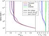 |
Fig. 4 Comparison of the non-irradiated solutions of the radiative transfer problem within the so-called picket-fence model approximation (see text). The left panel shows temperature (in Teff units) vs. optical depth. The right panel shows the relative temperature difference between our model and other works. The models shown correspond to the solutions of King (1955) (blue lines), Chandrasekhar (1935) (green lines), and this work (red lines). Different models correspond to the grey case (plain), i.e. R = 1, and 2 non-grey cases: β = 0.01, R = 103 (dashed) and β = 0.7, R = 103 (dotted) where R ≡ κ1/κ2. The red and green lines are so similar that they are almost indistinguishable in the left panel. |
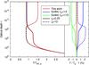 |
Fig. 5 Comparison between our model in the semi-grey limit and Guillot (2010). We used γv = 0.25
(plain line) and γv = 10 (dashed line). For the
Guillot (2010) model we show the curves for
two different boundary conditions:fH = 1/2 (blue) and fH = 1/ |
4.2. Comparison of irradiated solutions
The solutions presented in this work for the irradiated semi-grey case (i.e.
R ≡ κ1/κ2 = 1)
are very similar to those of Guillot (2010). As
seen in Fig. 5, the solutions obtained either with
fH = 1/2, or
 have relative differences of up to 2% with those of this work. These differences are of the same kind as
those arising from the use of the Eddington approximation compared to exact solutions
discussed previously. They are inherent to the approximation made on the angular
dependency of the radiation field and implicitly linked to the choice of the different
boundary conditions discussed in Sect. 2.3.2.
have relative differences of up to 2% with those of this work. These differences are of the same kind as
those arising from the use of the Eddington approximation compared to exact solutions
discussed previously. They are inherent to the approximation made on the angular
dependency of the radiation field and implicitly linked to the choice of the different
boundary conditions discussed in Sect. 2.3.2.
4.3. Comparison of skin temperatures
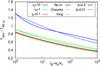 |
Fig. 6 Skin temperature of the planet given by our irradiated picket-fence model for
different values of γv and in the non-irradiated case.
Curves for β = 0.01 (plain lines) and β = 0.5 (dashed
lines) are shown. Skin temperature from Chandrasekhar
(1935) and King (1956) are also
shown. For the irradiated case we used |
As discussed previously, the skin temperature (temperature at the limit of zero optical
depth) is an important outcome of radiative transfer and in the case of non-irradiated
models, an exact solution is available. We compare our results to other analytical results
in Fig. 6. In the limit of a non-irradiated planet
and in the limit  , our
skin temperature converges to the one derived by Chandrasekhar (1935). This is an important test for the model, as for low values
of γv, most of the stellar flux is absorbed
in the deep layers of the planet and the model is expected to behave as a non-irradiated
model with the same effective temperature. Moreover, we note that for low values of
γv, the skin temperature is affected only
by γP as was already claimed by King (1956) and Chandrasekhar (1935). This conclusion no longer applies for higher values of
γv for which the skin temperature also
depends on β.
This can be seen by comparing the dotted lines and plain lines of the same colour in Fig.
6. At a given value of γP, a higher
value of β
corresponds to a smaller κ2/κ1.
Depending on the value of β, the stellar irradiation can be absorbed in a
region which can be optically thick to the two thermal bands, only one, or none, leading
to different behaviour for the skin temperature.
, our
skin temperature converges to the one derived by Chandrasekhar (1935). This is an important test for the model, as for low values
of γv, most of the stellar flux is absorbed
in the deep layers of the planet and the model is expected to behave as a non-irradiated
model with the same effective temperature. Moreover, we note that for low values of
γv, the skin temperature is affected only
by γP as was already claimed by King (1956) and Chandrasekhar (1935). This conclusion no longer applies for higher values of
γv for which the skin temperature also
depends on β.
This can be seen by comparing the dotted lines and plain lines of the same colour in Fig.
6. At a given value of γP, a higher
value of β
corresponds to a smaller κ2/κ1.
Depending on the value of β, the stellar irradiation can be absorbed in a
region which can be optically thick to the two thermal bands, only one, or none, leading
to different behaviour for the skin temperature.
5. Consequences of non-grey effects
In this section we study the physical processes that shape our non-grey temperature profile. To overcome the apparent complexity of our solution, we first derive an approximate expression for the thermal fluxes at the top of the atmosphere. We then obtain a much simpler expression for the skin and the deep temperatures. Comparing these expressions with their semi-grey equivalent, we get physical insights into the processes that shape the temperature profile.
5.1. Estimation of the fluxes in the different bands
In steady state, all the energy that penetrates the atmosphere must be radiated away. Thus, the radiative equilibrium at the top of the atmosphere is of great importance to understand how the non-grey effects shape the temperature profile. In particular, whether the thermal fluxes are transported by the channel of highest opacity (channel 1) or the channel of lowest opacity (channel 2) is of particular importance.
As seen in Eq. (76), the contribution to
the final temperature of the internal luminosity and of the external irradiation are
independent. Thus, the thermal fluxes can be split into two independent contributions that
can be studied separately:  (99)Figure 7 shows which thermal band actually carries the thermal
flux Hirr(0) out of the atmosphere (the flux
Firr(0) is equal to 4πHirr(0)). This depends
strongly on whether the stellar irradiation is absorbed in the upper or in the deep
atmosphere. If it is deposited in the deep layers of the planet (i.e. γv ≪ 1), most of
the flux is transported by the second thermal channel whatever the width of the
second channel. Conversely, when the stellar irradiation is deposited in the
upper atmosphere, most of the flux is carried by the first thermal channel
whatever the width of the first channel. The tipping point, i.e. when
each channel carries half of the flux, is reached when
(99)Figure 7 shows which thermal band actually carries the thermal
flux Hirr(0) out of the atmosphere (the flux
Firr(0) is equal to 4πHirr(0)). This depends
strongly on whether the stellar irradiation is absorbed in the upper or in the deep
atmosphere. If it is deposited in the deep layers of the planet (i.e. γv ≪ 1), most of
the flux is transported by the second thermal channel whatever the width of the
second channel. Conversely, when the stellar irradiation is deposited in the
upper atmosphere, most of the flux is carried by the first thermal channel
whatever the width of the first channel. The tipping point, i.e. when
each channel carries half of the flux, is reached when
 .
Figure 8 shows the variations of τlim with the
width and the strength of the two thermal opacity bands; τlim increases
with β but
decreases with R ≡ κ1/κ2.
It always corresponds to an optical depth where the first channel is optically thick and
the second is optically thin.
.
Figure 8 shows the variations of τlim with the
width and the strength of the two thermal opacity bands; τlim increases
with β but
decreases with R ≡ κ1/κ2.
It always corresponds to an optical depth where the first channel is optically thick and
the second is optically thin.
For high values of γP (i.e. γP > 2), we can
approximate the ratio of the thermal fluxes related to the irradiation by a much simpler
expression: 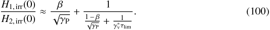 (100)As
shown in Fig. 7 this expression correctly matches the
expression of the analytical model. Depending on the value of
(100)As
shown in Fig. 7 this expression correctly matches the
expression of the analytical model. Depending on the value of
 , the expression
reduces to
, the expression
reduces to
 (101a)
 (101b)We
now look for a similar expression for the thermal fluxes resulting from the internal
luminosity (Hint). Because the internal luminosity
irradiates the atmosphere from below, the resulting thermal fluxes behave similarly to the
irradiated when γv → 0, thus we have
(101b)We
now look for a similar expression for the thermal fluxes resulting from the internal
luminosity (Hint). Because the internal luminosity
irradiates the atmosphere from below, the resulting thermal fluxes behave similarly to the
irradiated when γv → 0, thus we have  (102)As
γP is always greater than one and
β is always
lower than one, the internal luminosity is always transported by channel 2, the channel of
lowest opacity.
(102)As
γP is always greater than one and
β is always
lower than one, the internal luminosity is always transported by channel 2, the channel of
lowest opacity.
5.2. The skin temperature
The skin temperature reveals the behaviour of the atmosphere at low optical depths. This is the part of the atmosphere probed during the transit of an exoplanet in front of its host star and is therefore of particular importance to interpret the observations. Figure 9 shows that in the irradiated case non-grey effects always tend to lower the skin temperature compared to the semi-grey case. This upper atmospheric cooling is already significant (>10%) for slightly non-grey opacities (i.e. γP ≈ 2). For higher values of γP the cooling is stronger, reaching 50% for γP ≈ 10−1000. Conversely to the non-irradiated case, the skin temperature is not only a function of γP but also depends on β, i.e. not only are the mean opacities relevant, but also their actual shape. For high values of β, when the stellar irradiation is absorbed in the upper layers of the atmosphere (e.g. γv = 100) the cooling is more efficient than when the stellar irradiation is absorbed in the deep layers (e.g. γv = 0.01), whereas for low values of β the cooling is independent of γv.
The skin temperature results directly from the radiative equilibrium of the upper
atmosphere. Using the boundary condition (49)in the radiative equlibrium Eq. (23)evaluated at τ = 0 we can write  (103)where the skin
temperature is given by
(103)where the skin
temperature is given by  . The skin temperature,
depends on the values of H1(0) and H2(0) and thus
on whether the stellar irradiation is absorbed in the deep atmosphere or in the upper
atmosphere.
. The skin temperature,
depends on the values of H1(0) and H2(0) and thus
on whether the stellar irradiation is absorbed in the deep atmosphere or in the upper
atmosphere.
5.2.1. Case of deep absorption of the irradiation flux
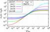 |
Fig. 7 Ratio of the total flux in the two thermal bands in function of
|
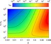 |
Fig. 8 Value of τlim in function of the width of the lines β and their strength κ1/κ2. The x-axis is in logit scale, where the function logit is defined as logit(x) = log (x/(1 − x)). |
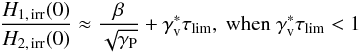
When  , the stellar irradiation is
absorbed in the deep layers of the atmosphere, where the second thermal band, the band
of lowest opacity, is optically thick. Thus, most of the flux is transported by the
second thermal band and we have H2(0) = H∞ − Hv(0).
For high values of γP, using Eq. (101)and Eq. (102)we get
, the stellar irradiation is
absorbed in the deep layers of the atmosphere, where the second thermal band, the band
of lowest opacity, is optically thick. Thus, most of the flux is transported by the
second thermal band and we have H2(0) = H∞ − Hv(0).
For high values of γP, using Eq. (101)and Eq. (102)we get  which is always larger than
one. Thus, although most of the flux is in the second thermal band, it is the first
band, the band of highest opacity, that sets the radiative equilibrium. Neglecting the
second term in Eq. (103)and calculating
H1(0) with Eqs. (101)and (102)we obtain:
which is always larger than
one. Thus, although most of the flux is in the second thermal band, it is the first
band, the band of highest opacity, that sets the radiative equilibrium. Neglecting the
second term in Eq. (103)and calculating
H1(0) with Eqs. (101)and (102)we obtain:
 (104)Noting that for high
values of γP,
(104)Noting that for high
values of γP,
 ,
and γ1 ≈ γP/β,
the equation becomes
,
and γ1 ≈ γP/β,
the equation becomes  (105)Replacing the fluxes by
their equivalent temperature we get an expression for the skin temperature valid for
and γP > 2:
(105)Replacing the fluxes by
their equivalent temperature we get an expression for the skin temperature valid for
and γP > 2:
 (106)When
, the first term dominates
and the expression differs by a factor of 1/
(106)When
, the first term dominates
and the expression differs by a factor of 1/ from the semi-grey case (Eq. (31)).
Because γP > 1 for
non-grey opacities, the skin temperature is always smaller in the non-grey case than in
the grey case, as shown in Fig. 9.
Physical interpretation. When
most of the irradiation is
absorbed where both thermal channels are optically thick. The flux is mainly transported
by the channel of lowest opacity κ2 but only the residual flux
transported by the channel of highest opacity κ1 contributes to the radiative
equilibrium at the top of the atmosphere. Because it represents only a small part of the
total flux, the upper atmosphere does not need to radiate a lot of energy and thus the
upper atmospheric temperatures are smaller than in the semi-grey case. The larger the
departure from the semi-grey opacities, the cooler the skin temperature, without lower
bounds.
from the semi-grey case (Eq. (31)).
Because γP > 1 for
non-grey opacities, the skin temperature is always smaller in the non-grey case than in
the grey case, as shown in Fig. 9.
Physical interpretation. When
most of the irradiation is
absorbed where both thermal channels are optically thick. The flux is mainly transported
by the channel of lowest opacity κ2 but only the residual flux
transported by the channel of highest opacity κ1 contributes to the radiative
equilibrium at the top of the atmosphere. Because it represents only a small part of the
total flux, the upper atmosphere does not need to radiate a lot of energy and thus the
upper atmospheric temperatures are smaller than in the semi-grey case. The larger the
departure from the semi-grey opacities, the cooler the skin temperature, without lower
bounds.
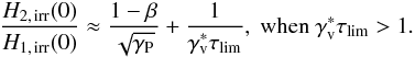
5.2.2. Case of shallow absorption of the irradiation flux
When  , most of the stellar
irradiation is absorbed in the upper atmosphere, where only the first thermal band is
optically thick. According to Eq. (101),
most of the flux originating from the irradiation Hirr(0) is
carried by the first thermal band, the band of highest opacity. Conversely, following
Eq. (102), the internal luminosity is
still transported by the second thermal channel, as in the γvτlim < 1
case. As γ1 > γ2,
the radiative equilibrium of the upper atmosphere is still determined by the channel of
highest opacity, channel 1, and the second term of Eq. (103)can be neglected. Conversely to the case γvτlim < 1,
the top boundary condition now reads H1(0) ≈ H1, int − Hv(0).
Using Eq. (102)to calculate
H1, int and noting
that for high values of γP, γP ≈ βγ1,
the radiative equilibrium becomes
, most of the stellar
irradiation is absorbed in the upper atmosphere, where only the first thermal band is
optically thick. According to Eq. (101),
most of the flux originating from the irradiation Hirr(0) is
carried by the first thermal band, the band of highest opacity. Conversely, following
Eq. (102), the internal luminosity is
still transported by the second thermal channel, as in the γvτlim < 1
case. As γ1 > γ2,
the radiative equilibrium of the upper atmosphere is still determined by the channel of
highest opacity, channel 1, and the second term of Eq. (103)can be neglected. Conversely to the case γvτlim < 1,
the top boundary condition now reads H1(0) ≈ H1, int − Hv(0).
Using Eq. (102)to calculate
H1, int and noting
that for high values of γP, γP ≈ βγ1,
the radiative equilibrium becomes
 (107)Replacing the fluxes by
their equivalent temperatures we get an expression for the skin temperature valid for
and γP > 2
(107)Replacing the fluxes by
their equivalent temperatures we get an expression for the skin temperature valid for
and γP > 2 (108)This
relation differs from the case as the factor
1/
before the irradiation temperatures is replaced by a factor 1/β. Thus, the skin
temperature no longer becomes arbitrarily low. However, for high values of
γv, the second term in the parenthesis
dominates and the skin temperature decreases proportionally to 1/,
which is faster than in the case . As an example, in Fig.
9, for γv = 100, the skin temperature
decreases much faster when γP increases for large values of
β (i.e.
when ).
Physical interpretation. When
, most of the incident
irradiation is absorbed in the upper atmosphere, where the second channel is optically
thin. Therefore it is mainly transported by the channel of highest opacity: channel 1.
Similarly to the case , the radiative equilibrium
at the top of the atmosphere is set by the channel of highest opacity, the one that
carries most of the thermal flux. Therefore all the flux from the irradiation
contributes to the radiative equilibrium of the upper layers and the skin temperature
cannot cool as much as in the case, its lowest value
being
(108)This
relation differs from the case as the factor
1/
before the irradiation temperatures is replaced by a factor 1/β. Thus, the skin
temperature no longer becomes arbitrarily low. However, for high values of
γv, the second term in the parenthesis
dominates and the skin temperature decreases proportionally to 1/,
which is faster than in the case . As an example, in Fig.
9, for γv = 100, the skin temperature
decreases much faster when γP increases for large values of
β (i.e.
when ).
Physical interpretation. When
, most of the incident
irradiation is absorbed in the upper atmosphere, where the second channel is optically
thin. Therefore it is mainly transported by the channel of highest opacity: channel 1.
Similarly to the case , the radiative equilibrium
at the top of the atmosphere is set by the channel of highest opacity, the one that
carries most of the thermal flux. Therefore all the flux from the irradiation
contributes to the radiative equilibrium of the upper layers and the skin temperature
cannot cool as much as in the case, its lowest value
being  . However, for high values
of and as long
as
. However, for high values
of and as long
as  ,
,
 decreases
faster than in the case . This confines the
stratosphere due to
decreases
faster than in the case . This confines the
stratosphere due to  (i.e.
the atmospheric levels with a temperature inversion) around the τ = τlim level whereas
it extends up to τ = 0 in the semi-grey case (see Figs. 12−14 hereafter).
(i.e.
the atmospheric levels with a temperature inversion) around the τ = τlim level whereas
it extends up to τ = 0 in the semi-grey case (see Figs. 12−14 hereafter).
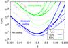 |
Fig. 9 Contours of the relative difference between the skin temperature in the non-grey
model and in the semi-grey model for different values of γv in
function of the width of the lines and their strength. The non-grey atmosphere is
10% (resp.
50%) cooler than the
semi-grey atmosphere above the blue (resp. green) lines. The dashed lines are
contours of γP. We used μ∗ = 1/ |
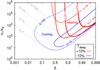 |
Fig. 10 Contours of the relative difference between the deep temperature in the non-grey
model and in the semi-grey model for different values of γv in
function of the width of the lines and their strength. The non-grey atmosphere is
10% hotter (resp.
cooler) than the semi-grey atmosphere inside the red (resp. blue) contours. The
dashed lines are contours of γP. We used μ∗ = 1/ |
5.3. The deep temperature
The temperature of the deep atmosphere is a fundamental outcome from radiative transfer
models as it reveals the energy exchange between the planet and its surroundings.
Therefore, it is often used as a boundary condition of planetary interior models. We
define the deep temperature as  (109)Thus, the
temperature of the deep atmosphere can be approximated as
(109)Thus, the
temperature of the deep atmosphere can be approximated as
 between the τ ≈ 1 level and the
radiative/convective boundary. For irradiated planets, the deep temperature corresponds to
the isothermal zone around τ ≈ 1 and is close to the temperature at
10 bar often used as a
boundary condition for interior models (e.g., Burrows et
al. 1997; Guillot & Showman 2002).
As seen in Fig. 10, the deep temperature has a
complex behaviour. For low values of γv, whenever β becomes large enough, the
deep temperature increases compared to the semi-grey case, an effect known as the
line blanketing effect in the stellar literature (e.g. Milne 1921; Chandrasekhar 1935; Hubeny & Lanz
1995). This effect is always maximum when
between the τ ≈ 1 level and the
radiative/convective boundary. For irradiated planets, the deep temperature corresponds to
the isothermal zone around τ ≈ 1 and is close to the temperature at
10 bar often used as a
boundary condition for interior models (e.g., Burrows et
al. 1997; Guillot & Showman 2002).
As seen in Fig. 10, the deep temperature has a
complex behaviour. For low values of γv, whenever β becomes large enough, the
deep temperature increases compared to the semi-grey case, an effect known as the
line blanketing effect in the stellar literature (e.g. Milne 1921; Chandrasekhar 1935; Hubeny & Lanz
1995). This effect is always maximum when  (see Fig. 8). Conversely, for high values of
(i.e.
(see Fig. 8). Conversely, for high values of
(i.e.
 ), the
deep atmosphere warms up only for high values of γP
(
), the
deep atmosphere warms up only for high values of γP
( ) whereas it
becomes cooler than in the semi-grey case for lower values of γP, a behaviour
that was not spotted in previous analytical models.
) whereas it
becomes cooler than in the semi-grey case for lower values of γP, a behaviour
that was not spotted in previous analytical models.
The deep atmospheric temperature is directly set by the boundary condition at the top of
the atmosphere. From Eq. (58), we see that
when τ → ∞,
 (110)where C1 is set by the
top boundary condition (49)applied on
Jγ(0) (see Eq. (52)):
(110)where C1 is set by the
top boundary condition (49)applied on
Jγ(0) (see Eq. (52)):
 (111)Similarly to the skin
temperature, the deep temperature depends on H1(0) and H2(0), and also
depends on whether the thermal flux is transported by the first or by the second thermal
channel, i.e. whether γvτlim is
larger or smaller than one.
(111)Similarly to the skin
temperature, the deep temperature depends on H1(0) and H2(0), and also
depends on whether the thermal flux is transported by the first or by the second thermal
channel, i.e. whether γvτlim is
larger or smaller than one.
5.3.1. Case of deep absorption of the irradiation flux
In the case , most of the thermal flux
is transported by the second thermal channel and because γ1 ≫ γ2 we
can write  (112)applying the
radiative equilibrium at the top of the atmosphere, and considering that most of the
flux is carried by the second thermal channel, we get
(112)applying the
radiative equilibrium at the top of the atmosphere, and considering that most of the
flux is carried by the second thermal channel, we get
 (113)Thus, we can
calculate C1 and obtain
(113)Thus, we can
calculate C1 and obtain
 (114)For high values of
γP, γ2 ≈ (1 − β). Replacing
the fluxes by their equivalent temperatures we get an expression for Tdeep valid
for and γP > 2:
(114)For high values of
γP, γ2 ≈ (1 − β). Replacing
the fluxes by their equivalent temperatures we get an expression for Tdeep valid
for and γP > 2:
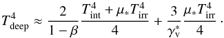 (115)This
expression differs from the semi-grey value of Guillot
(2010) by a factor 1/(1 − β) multiplying the
first term. Thus, when β → 1, the temperature becomes warmer than in the
semi-grey case, as seen for the low values of γv in Fig. 10. Physical interpretation. When
, most of the flux from the
star is absorbed in the deep atmosphere and is principally transported by the channel of
lowest opacity (channel 2), even when the width of this channel is smaller than the
width of the first thermal channel. Whenever β → 1, the width of the second channel decreases.
In order to keep transporting most of the thermal flux, the flux per wavelength in the
second channel must increase. This increases the temperature where the second channel is
optically thick, i.e. in the deep atmosphere. This is equivalent to the line
blanketing effect that has been well studied in stars (see Milne 1921; Chandrasekhar 1935; Hubeny & Lanz
1995, for example).
(115)This
expression differs from the semi-grey value of Guillot
(2010) by a factor 1/(1 − β) multiplying the
first term. Thus, when β → 1, the temperature becomes warmer than in the
semi-grey case, as seen for the low values of γv in Fig. 10. Physical interpretation. When
, most of the flux from the
star is absorbed in the deep atmosphere and is principally transported by the channel of
lowest opacity (channel 2), even when the width of this channel is smaller than the
width of the first thermal channel. Whenever β → 1, the width of the second channel decreases.
In order to keep transporting most of the thermal flux, the flux per wavelength in the
second channel must increase. This increases the temperature where the second channel is
optically thick, i.e. in the deep atmosphere. This is equivalent to the line
blanketing effect that has been well studied in stars (see Milne 1921; Chandrasekhar 1935; Hubeny & Lanz
1995, for example).
5.3.2. Case of shallow absorption of the irradiation flux
When most of the irradiation
flux is absorbed in a region where the second thermal channel is optically thin. Thus
the flux is carried by the first thermal channel and we have H1, irr(0) ≫ H2, irr(0).
However, because γ2 ≪ γ1,
we can use Eq. (101b) to show that  , which is larger than 1.
Thus Eq. (112)remains valid. However,
conversely to the case , the top boundary condition
now reads
, which is larger than 1.
Thus Eq. (112)remains valid. However,
conversely to the case , the top boundary condition
now reads 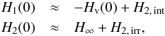 (116)where
H2, irr is given by
Eq. (101b) and H1, int by Eq.
(102). This leads to:
(116)where
H2, irr is given by
Eq. (101b) and H1, int by Eq.
(102). This leads to:
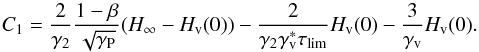 (117)Again, for large values
of γP, γ2 → 1 − β and
replacing the fluxes by their equivalent temperatures we get an expression for
Tdeep valid for
and γP > 2:
(117)Again, for large values
of γP, γ2 → 1 − β and
replacing the fluxes by their equivalent temperatures we get an expression for
Tdeep valid for
and γP > 2:
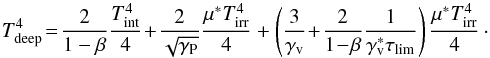 (118)When
 , the contribution to the
deep temperature of the irradiation temperature becomes inversely proportional to
, the contribution to the
deep temperature of the irradiation temperature becomes inversely proportional to
 .
As γP > 1, the
deep temperature is smaller in the non-grey case than in the semi-grey case. This is
illustrated by the cases γv = 10 and γv = 100 in
Fig. 10. When
.
As γP > 1, the
deep temperature is smaller in the non-grey case than in the semi-grey case. This is
illustrated by the cases γv = 10 and γv = 100 in
Fig. 10. When
 , the term in
 becomes very small compared to the term in 1/(1 − β) and the expression
converges toward equation Eq. (115),
valid for . Physical
interpretation. When , the incident irradiation
is absorbed in the upper atmosphere, where only the channel of highest opacity is
optically thick. Thus, the channel of highest opacity κ1 transports
all the energy and radiates it directly to space. The incident irradiation is no more
transported to the deep atmosphere, leading to a cooler deep atmosphere.
becomes very small compared to the term in 1/(1 − β) and the expression
converges toward equation Eq. (115),
valid for . Physical
interpretation. When , the incident irradiation
is absorbed in the upper atmosphere, where only the channel of highest opacity is
optically thick. Thus, the channel of highest opacity κ1 transports
all the energy and radiates it directly to space. The incident irradiation is no more
transported to the deep atmosphere, leading to a cooler deep atmosphere.
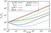 |
Fig. 11 Ratio of the monochromatic flux in the two bands Fν2/Fν1 = βH2(0)/(1 − β)H1(0)
in function of the opacity ratio κ1/κ2
for different bandwidths β and visible to infrared opacities
γv. We used
|
5.4. Outgoing flux
During secondary eclipse observations, the flux emitted by the planet can be observed in
different bands (e.g. Seager & Deming
2010). The detection of molecular species in the emission spectrum of an exoplanet
depends strongly on the flux contrast between the continuum and the molecular band
considered, which in turn depends on the temperature profile. Figure 11 shows the flux per wavelength emitted in the first band
(Fν1 = 4πH1(0)/β)
over the flux per wavelength emitted in the second band (Fν2 = 4πH2(0)/(1 − β)).
This would be the expected contrast in the emission spectrum of the planet between the
spectral features and the continuum. For a non-irradiated atmosphere and for low values of
γv this is a monotonic function of the
opacity ratio κ1/κ2.
The flux in the band of lowest opacity is always bigger than the flux in the band of
highest opacity, i.e. we see absorption bands. For large values of γv, whenever a
strong temperature inversion happens the absorption bands turn into emission bands. Those
different behaviours are captured by the simple expression (100). Note that in all cases, for large values of κ1/κ2
we have: 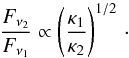 (119)
(119)
6. Resulting temperature profiles
No matter how strong the non-greyness of the opacities is, there is always a region, at high enough optical depth, where the non-grey solution converges toward the grey solution (see e.g. Fig. 4). The transition between a regime where the grey model is accurate to a regime where the non-grey effects are of prime importance is set by the parameter τlim. For optical depths lower than τlim, non-grey effects are always important, whereas for optical depths higher than τlim, non-grey effects are present only if γvτlim < 1 and β → 1. Three distinct situations can be observed in Fig. 8. For narrow lines (β < 0.1), τlim is always smaller than one, for larger lines or molecular bands (0.1 < β < 0.9), τlim is close to one, whereas for inverted lines (0.9 < β < 1), τlim can reach much higher values. Thus, when γv ≫ 1, few non-grey effects are expected in the deep atmosphere, contrary to the cases γv ≈ 1 and γv ≪ 1.
In the case of narrow lines (β < 0.1), only the non-grey cooling of the upper atmosphere is effective. As shown in Fig. 12, the profile remains close to the semi-grey model at large optical depths. However, at low optical depths, for τ < τlim, the atmosphere can be much cooler than in the semi-grey case (case R = 1). In particular, in the γv = 10 case, the non-grey cooling localizes the temperature inversion to a specific layer, contrary to the semi-grey case where it extends to the top of the atmosphere. The envelope of all the profiles (shaded area) is much wider than in the semi-grey case (see Fig. 1).
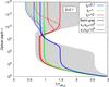 |
Fig. 12 Pressure/temperature profiles for an irradiated planet (Tint = Tirr/10
and μ∗ = 1/ |
In the case of large lines or molecular bands (0.1 < β < 0.9)
shown in Fig. 13, both the non-grey cooling of the
upper atmosphere and the blanketing effect are important. Whereas the upper atmosphere
undergoes an efficient cooling, the lower atmosphere (τ > 1) can experience a
significant warming via the blanketing effect. Lowering the ability of the deep atmosphere
to cool down efficiently can significantly affect the evolution of the planet (Parmentier & Guillot 2011; Budaj et al. 2012; Spiegel &
Burrows 2013; Rauscher & Showman
2013) and could contribute to the radius anomaly of hot-Jupiters (e.g. Guillot & Showman 2002; Laughlin et al. 2011). Whenever  , the stellar irradiation is
deposited at a level where non-grey effects lower the ability of the atmosphere to cool down
efficiently. This leads to an efficient and localized warming causing a temperature
inversion in the profile at
, the stellar irradiation is
deposited at a level where non-grey effects lower the ability of the atmosphere to cool down
efficiently. This leads to an efficient and localized warming causing a temperature
inversion in the profile at  , even when
none is expected from the semi-grey model (i.e. even when
, even when
none is expected from the semi-grey model (i.e. even when
 ). This
happens, for example, when β ≈ 0.5 for γv = 10, when β ≈ 0.9 for γv = 1, and for
β ≈ 0.99 for
γv = 0.1 (see Fig. 14).
). This
happens, for example, when β ≈ 0.5 for γv = 10, when β ≈ 0.9 for γv = 1, and for
β ≈ 0.99 for
γv = 0.1 (see Fig. 14).
In the case of inverted lines (β > 0.9), shown in Fig. 14, both the upper temperature and the deep temperature are affected by the non-grey effects. The upper atmosphere cools significantly compared to the semi-grey case. The deep atmosphere can either warm up because of the blanketing effect but, for high values of γv it can also become cooler than in the semi-grey case (see the case γv = 10 and R = 100 in Fig. 14). Temperatures as cool as 0.5Teff, μ∗ can be reached. This is fundamentally different from the semi-grey case where the deep temperature is always larger than 21/4Teff, μ∗ (see Fig. 3).
As β increases, τlim increases and the blanketing effect disappears. Eventually, when β → 1, the opacities, and thus the profile, become semi-grey again.
In summary, our irradiated picket-fence model can reach the whole temperature range span by the numerical models (see the shaded area in Figs. 12 to 14). Our model should therefore be preferred to classical semi-grey models as an approximate solution for the temperature profile of irradiated atmospheres.
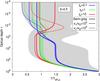 |
Fig. 13 Pressure/temperature profiles for an irradiated planet (Tint = Tirr/10
and μ∗ = 1/ |
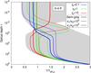 |
Fig. 14 Pressure/temperature profiles for an irradiated planet (Tint = Tirr/10
and μ∗ = 1/ |
Main quantities used in this paper.
7. Conclusion
We derived an analytic non-grey model to approximate the structure of a plane-parallel irradiated planetary atmosphere. Our model includes both thermal and visible non-grey opacities. The thermal and visible opacities are in the form of a two different picket-fence opacity functions. the thermal opacities are parametrized by the ratio of the visible to the infrared Rosseland mean opacities (γv), the ratio of the Planck to the Rosseland mean thermal opacities (γP), and the spectral width of the lines (β). The model is valid for any functional form of the Rosseland mean opacities, the ones obtained from an opacity table for example. However, it cannot account for both realistic Rosseland mean and Planck mean opacities. Their ratio, γP and the width of the lines, β, must be held constant through the atmosphere. Although the model is limited to two thermal opacity bands, it can take into account any number of visible opacity bands, each band adding two new parameters, the strength of the band γvi and its width βvi Our model solves the inability of previous analytical models to reach temperatures as cold as predicted by the numerical calculations. For opacities dominated by strong and narrow lines (β < 0.1), non-grey opacities lead to a colder upper atmosphere, but converges toward the grey model at optical depth greater than τlim (see Fig. 8). For opacities dominated by wide lines, or molecular bands (β ≈ 0.5), non-grey opacities still allow the upper atmosphere to cool down more efficiently, but also inhibit the cooling of the deep atmosphere. In that case, a significant warming of the deep atmosphere can happen, down to optical depths much greater than τlim. This planetary blanketing effect could contribute to the radius anomaly of hot Jupiters.
Temperature inversions that were not predicted by previous analytical models occur whenever
 because of the interaction between
the incoming stellar irradiation and the non-grey thermal opacities. These could have
interesting observational consequences.
because of the interaction between
the incoming stellar irradiation and the non-grey thermal opacities. These could have
interesting observational consequences.
We show that the internal flux is always transported by the spectral channel of lowest
opacity. Conversely, the absorbed irradiation flux is transported by the spectral channel of
lowest opacity only when . For values of
larger than
 ,
it is transported by the spectral channel of highest opacity.We provide simple analytical
expressions for the outgoing thermal flux in the different spectral bands.
,
it is transported by the spectral channel of highest opacity.We provide simple analytical
expressions for the outgoing thermal flux in the different spectral bands.
Finally, our model allows for a much greater range of temperature profiles than other analytical and semi-analytical solutions of the radiative transfer equations for irradiated atmospheres. We encourage the community to use it when fast calculations of atmospheric temperature profiles are needed. Given the apparent complexity of the solution, a code is available at the CDS or at www.oca.eu/parmentier/nongrey.
In stellar physics the effective temperature is usually what we call the internal
temperature. In both planetary and stellar fields, the effective temperature aims at
representing the total energy budget of the atmosphere. Although in stellar physics most
of the flux comes from the deep interior, this is not true in irradiated atmospheres, and
 is a better
representation of the total energy budget of the studied slice of atmosphere. The energy
budget of the whole atmosphere is therefore
is a better
representation of the total energy budget of the studied slice of atmosphere. The energy
budget of the whole atmosphere is therefore  .
.
We noticed that the values of L1 and L3 in Chandrasekhar’s book were inverted and corrected this here.
Acknowledgments
This work was performed in part thanks to a joint Fulbright Fellowship to V.P. and T.G. The whole project would not have been possible without the help and support of Douglas Lin. We also acknowledge Jonathan Fortney and Mark Marley for many useful discussions, and the University of California Santa Cruz for hosting us while this work was carried out.
References
- Avrett, E. H., & Krook, M. 1963, ApJ, 137, 874 [NASA ADS] [CrossRef] [Google Scholar]
- Budaj, J., Hubeny, I., & Burrows, A. 2012, A&A, 537, A115 [NASA ADS] [CrossRef] [EDP Sciences] [Google Scholar]
- Burrows, A., Marley, M., Hubbard, W. B., et al. 1997, ApJ, 491, 856 [NASA ADS] [CrossRef] [Google Scholar]
- Burrows, A., Hubeny, I., Budaj, J., Knutson, H. A., & Charbonneau, D. 2007, ApJ, 668, L171 [NASA ADS] [CrossRef] [MathSciNet] [Google Scholar]
- Chandrasekhar, S. 1935, MNRAS, 96, 21 [NASA ADS] [Google Scholar]
- Chandrasekhar, S. 1960, Radiative transfer (New york: Dover Publications) [Google Scholar]
- Chevallier, L., Pelkowski, J., & Rutily, B. 2007, J. Quant. Spectr. Radiat. Transf., 104, 357 [NASA ADS] [CrossRef] [Google Scholar]
- Eddington, A. S. 1916, MNRAS, 77, 16 [NASA ADS] [Google Scholar]
- Fortney, J. J., Lodders, K., Marley, M. S., & Freedman, R. S. 2008, ApJ, 678, 1419 [NASA ADS] [CrossRef] [Google Scholar]
- Guillot, T. 2010, A&A, 520, A27 [NASA ADS] [CrossRef] [EDP Sciences] [Google Scholar]
- Guillot, T., & Havel, M. 2011, A&A, 527, A20 [NASA ADS] [CrossRef] [EDP Sciences] [Google Scholar]
- Guillot, T., & Showman, A. P. 2002, A&A, 385, 156 [NASA ADS] [CrossRef] [EDP Sciences] [Google Scholar]
- Hansen, B. M. S. 2008, ApJS, 179, 484 [NASA ADS] [CrossRef] [Google Scholar]
- Heng, K., Menou, K., & Phillipps, P. J. 2011, MNRAS, 413, 2380 [NASA ADS] [CrossRef] [Google Scholar]
- Heng, K., Hayek, W., Pont, F., & Sing, D. K. 2012, MNRAS, 420, 20 [NASA ADS] [CrossRef] [Google Scholar]
- Hubeny, I., & Lanz, T. 1995, ApJ, 439, 875 [Google Scholar]
- Hubeny, I., Burrows, A., & Sudarsky, D. 2003, ApJ, 594, 1011 [NASA ADS] [CrossRef] [Google Scholar]
- King, I. J. I. F. 1955, ApJ, 121, 711 [NASA ADS] [CrossRef] [Google Scholar]
- King, J. I. F. 1956, ApJ, 124, 272 [NASA ADS] [CrossRef] [Google Scholar]
- Krook, M. 1963, ApJ, 137, 863 [NASA ADS] [CrossRef] [Google Scholar]
- Laughlin, G., Crismani, M., & Adams, F. C. 2011, ApJ, 729, L7 [NASA ADS] [CrossRef] [Google Scholar]
- Line, M. R., Zhang, X., Vasisht, G., et al. 2012, ApJ, 749, 93 [NASA ADS] [CrossRef] [Google Scholar]
- Matsui, T., & Abe, Y. 1986, Nature, 322, 526 [NASA ADS] [CrossRef] [Google Scholar]
- Meador, W. E., & Weaver, W. R. 1980, Journal of Atmospheric Sciences, 37, 630 [Google Scholar]
- Mihalas, D. 1978, Stellar atmospheres, 2nd edn. (W.H. Freeman and Co.) [Google Scholar]
- Mihalas, D., & Mihalas, B. W. 1984, Foundations of radiation hydrodynamics (New york: Oxford University Press) [Google Scholar]
- Miller-Ricci, E., & Fortney, J. J. 2010, ApJ, 716, L74 [NASA ADS] [CrossRef] [Google Scholar]
- Milne, E. A. 1921, MNRAS, 81, 510 [NASA ADS] [Google Scholar]
- Mordasini, C., Alibert, Y., Georgy, C., et al. 2012a, A&A, 547, A112 [NASA ADS] [CrossRef] [EDP Sciences] [Google Scholar]
- Mordasini, C., Alibert, Y., Klahr, H., & Henning, T. 2012b, A&A, 547, A111 [NASA ADS] [CrossRef] [EDP Sciences] [Google Scholar]
- Münch, G. 1946, ApJ, 104, 87 [NASA ADS] [CrossRef] [Google Scholar]
- Parmentier, V., & Guillot, T. 2011, in EPSC-DPS Joint Meeting 2011, 1367 [Google Scholar]
- Pierrehumbert, R. T. 2010, Principles of Planetary Climate (Cambridge: University Press) [Google Scholar]
- Pujol, T., & North, G. R. 2003, Tellus A, 55, 328 [NASA ADS] [CrossRef] [Google Scholar]
- Rauscher, E., & Menou, K. 2013, ApJ, 764, 103 [NASA ADS] [CrossRef] [Google Scholar]
- Rauscher, E., & Showman, A. P. 2013, ApJ, submitted [arXiv:1309.7052] [Google Scholar]
- Robinson, T. D., & Catling, D. C. 2012, ApJ, 757, 104 [NASA ADS] [CrossRef] [Google Scholar]
- Rutily, B., Chevallier, L., Pelkowski, J., & Bergeat, J. 2008, J. Quant. Spectr. Radiat. Transf., 109, 28 [NASA ADS] [CrossRef] [Google Scholar]
- Saumon, D., Hubbard, W. B., Burrows, A., et al. 1996, ApJ, 460, 993 [NASA ADS] [CrossRef] [Google Scholar]
- Seager, S., & Deming, D. 2010, ARA&A, 48, 631 [NASA ADS] [CrossRef] [Google Scholar]
- Shaviv, N. J., Shaviv, G., & Wehrse, R. 2011, Icarus, 216, 403 [NASA ADS] [CrossRef] [Google Scholar]
- Showman, A. P., Fortney, J. J., Lian, Y., et al. 2009, ApJ, 699, 564 [NASA ADS] [CrossRef] [Google Scholar]
- Spiegel, D. S., & Burrows, A. 2013, ApJ, 772, 76 [NASA ADS] [CrossRef] [Google Scholar]
- Unno, W., & Yamashita, Y. 1960, PASJ, 12, 157 [NASA ADS] [Google Scholar]
- Weaver, C. P., & Ramanathan, V. 1995, J. Geophys. Res., 100, 11585 [NASA ADS] [CrossRef] [Google Scholar]
All Tables
All Figures
|
Fig. 1 Optical depth vs. atmospheric temperature in units of the effective temperature. A
numerical solution obtained from Fortney et al.
(2008) (thick black line) is compared to the semi-grey analytical solutions
of Guillot (2010) for values of the greenhouse
factor |
| In the text | |
|
Fig. 2 Simplified thermal opacities for the picket-fence model. β = δν/Δν is the equivalent bandwidth (see text). |
| In the text | |
|
Fig. 3 Minimum temperature of the semi-grey model in terms of the effective temperature as a function of γv/μ∗. |
| In the text | |
|
Fig. 4 Comparison of the non-irradiated solutions of the radiative transfer problem within the so-called picket-fence model approximation (see text). The left panel shows temperature (in Teff units) vs. optical depth. The right panel shows the relative temperature difference between our model and other works. The models shown correspond to the solutions of King (1955) (blue lines), Chandrasekhar (1935) (green lines), and this work (red lines). Different models correspond to the grey case (plain), i.e. R = 1, and 2 non-grey cases: β = 0.01, R = 103 (dashed) and β = 0.7, R = 103 (dotted) where R ≡ κ1/κ2. The red and green lines are so similar that they are almost indistinguishable in the left panel. |
| In the text | |
|
Fig. 5 Comparison between our model in the semi-grey limit and Guillot (2010). We used γv = 0.25
(plain line) and γv = 10 (dashed line). For the
Guillot (2010) model we show the curves for
two different boundary conditions:fH = 1/2 (blue) and fH = 1/ |
| In the text | |
|
Fig. 6 Skin temperature of the planet given by our irradiated picket-fence model for
different values of γv and in the non-irradiated case.
Curves for β = 0.01 (plain lines) and β = 0.5 (dashed
lines) are shown. Skin temperature from Chandrasekhar
(1935) and King (1956) are also
shown. For the irradiated case we used |
| In the text | |
|
Fig. 7 Ratio of the total flux in the two thermal bands in function of
|
| In the text | |
|
Fig. 8 Value of τlim in function of the width of the lines β and their strength κ1/κ2. The x-axis is in logit scale, where the function logit is defined as logit(x) = log (x/(1 − x)). |
| In the text | |
|
Fig. 9 Contours of the relative difference between the skin temperature in the non-grey
model and in the semi-grey model for different values of γv in
function of the width of the lines and their strength. The non-grey atmosphere is
10% (resp.
50%) cooler than the
semi-grey atmosphere above the blue (resp. green) lines. The dashed lines are
contours of γP. We used μ∗ = 1/ |
| In the text | |
|
Fig. 10 Contours of the relative difference between the deep temperature in the non-grey
model and in the semi-grey model for different values of γv in
function of the width of the lines and their strength. The non-grey atmosphere is
10% hotter (resp.
cooler) than the semi-grey atmosphere inside the red (resp. blue) contours. The
dashed lines are contours of γP. We used μ∗ = 1/ |
| In the text | |
|
Fig. 11 Ratio of the monochromatic flux in the two bands Fν2/Fν1 = βH2(0)/(1 − β)H1(0)
in function of the opacity ratio κ1/κ2
for different bandwidths β and visible to infrared opacities
γv. We used
|
| In the text | |
|
Fig. 12 Pressure/temperature profiles for an irradiated planet (Tint = Tirr/10
and μ∗ = 1/ |
| In the text | |
|
Fig. 13 Pressure/temperature profiles for an irradiated planet (Tint = Tirr/10
and μ∗ = 1/ |
| In the text | |
|
Fig. 14 Pressure/temperature profiles for an irradiated planet (Tint = Tirr/10
and μ∗ = 1/ |
| In the text | |
Current usage metrics show cumulative count of Article Views (full-text article views including HTML views, PDF and ePub downloads, according to the available data) and Abstracts Views on Vision4Press platform.
Data correspond to usage on the plateform after 2015. The current usage metrics is available 48-96 hours after online publication and is updated daily on week days.
Initial download of the metrics may take a while.