| Issue |
A&A
Volume 562, February 2014
|
|
|---|---|---|
| Article Number | A144 | |
| Number of page(s) | 10 | |
| Section | Extragalactic astronomy | |
| DOI | https://doi.org/10.1051/0004-6361/201322267 | |
| Published online | 24 February 2014 | |
The dependency of AGN infrared colour-selection on source luminosity and obscuration
An observational perspective in CDFS and COSMOS
1
Centro de Astronomia e Astrofísica da Universidade de Lisboa, Observatório
Astronómico de Lisboa,
Tapada da Ajuda,
1349-018
Lisboa,
Portugal
e-mail:
This email address is being protected from spambots. You need JavaScript enabled to view it.
2
Departamento de Astronomía, Av. Esteban Iturra 6to piso, Facultad
de Ciencias Físicas y Matemáticas, Universidad de Concepción,
4009
Casilla,
Chile
3
Max Planck for Extraterrestrial Physics, Giessembachstrasse 1,
85748
Garching,
Germany
4
Excellence Cluster, Boltzmann Strasse 2,
85748
Garching,
Germany
5
University of California, 900 University Ave.,
Riverside
CA
92521,
USA
6
Australian Astronomical Observatory, PO Box 915, North Ryde
NSW
1670,
Australia
Received:
11
July
2013
Accepted:
2
December
2013
Abstract
Aims. This work addresses the AGN IR-selection dependency on intrinsic source luminosity and obscuration, in order to identify and characterise biases that could affect conclusions in studies.
Methods. We study IR-selected AGN in the Chandra Deep Field South (CDFS) survey and in the Cosmological Survey (COSMOS). The AGN sample is divided into low and high X-ray luminosity classes and into unobscured (type-1) and obscured (type-2) classes by means of X-ray and optical spectroscopy data. Specifically in the X-ray regime, we adopt the intrinsic luminosity taking the estimated column density (NH) into account. We also take the opportunity to highlight important differences resulting from adopting different methods of assessing AGN obscuration.
Results. In agreement with previous studies, we also find that AGN IR-selection efficiency shows a decrease with decreasing source AGN X-ray luminosity. For the intermediate-luminosity AGN population (43.3 ≲ log (LX [erg s-1] ) ≲ 44), the efficiency also worsens with increasing obscuration (NH). The same sample also shows an evolution with cosmic time of the obscured fraction at the highest X-ray luminosities, independently of the adopted type-1/type-2 classification method.
Conclusions. We confirm that AGN IR-selection is genuinely biased towards unobscured AGNe, but only at intermediate luminosities. At the highest luminosities, where AGN IR-selection is more efficient, there is no obscuration bias. We show that type-1 AGNe are intrinsically more luminous than type-2 AGNe only at z ≲ 1.6, thus resulting in more type-1 AGN being selected when the IR survey is shallower. Based on this and other studies, we conclude that deep hard-X-ray coverages, high-resolution IR imaging, or a combination of IR and radio data are required to recover the lower luminosity obscured AGN population. In addition, wide IR surveys are needed to recover the rare powerful, obscured AGN population. Finally, when the James Webb Space Telescope comes online, the broad-band filters 2.0 μm, 4.4 μm, 7.7 μm, and 18 μm will be essential for disentangling AGN from non-AGN dominated SEDs at depths where spectroscopy becomes impractical.
Key words: galaxies: active / galaxies: evolution / galaxies: nuclei / galaxies: statistics / infrared: galaxies / X-rays: galaxies
© ESO, 2014
1. Introduction
It is believed today that there is a significant fraction of obscured active galactic nuclei (AGN) that still remain unidentified at high-energy spectral-bands even in the current deepest surveys (the strongest evidence coming from X-ray studies, e.g., Comastri et al. 2001; Ueda et al. 2003; Gilli 2004; Worsley et al. 2004, 2005; Treister & Urry 2005; Martínez-Sansigre et al. 2005; Draper & Ballantyne 2009; Burlon et al. 2011; Ajello et al. 2012; Moretti et al. 2012). With an incomplete demography of actively accreting super-massive black holes, current galaxy evolution models accounting for AGN feedback (e.g., Granato et al. 2004; Springel et al. 2005; Croton et al. 2006; Hopkins et al. 2006; Bower et al. 2006; Somerville et al. 2008) probably remain poorly constrained. As a result, alternative means of finding such objects by different spectral regimes ought to be developed.
If high dust column densities are the driver for such extreme obscuration of direct light from the AGN accretion region (instead of just obscuring circumnuclear gas clouds), then infrared (IR) wavelengths, at which the obscuring dust emits (e.g., Nenkova et al. 2008; Hönig & Kishimoto 2010), are an obvious choice in the search for such extreme objects. Hints of AGN activity at IR wavelengths can be revealed through spectroscopy diagnostics (Laurent et al. 2000; Armus et al. 2007; Veilleux et al. 2009) or photometric techniques. The latter encompass the selection of AGN-like sources by means of1 colour−colour constraints (de Grijp et al. 1985; Miley et al. 1985; Lacy et al. 2004, 2007; Hatziminaoglou et al. 2005, 2010; Stern et al. 2005; Assef et al. 2010, 2013; Hony et al. 2011; Jarrett et al. 2011; Donley et al. 2012; Mateos et al. 2012; Messias et al. 2012), red power-law spectral energy distribution (SED) fitting (Alonso-Herrero et al. 2006; Donley et al. 2007), excess IR emission unmatched by pure star-forming SEDs (Daddi et al. 2007), or large optical-to-IR flux ratios (f24/fR > 1000), in addition to bright IR flux cuts and/or extremely red optical-to-near-IR colour cuts (Dey et al. 2008; Fiore et al. 2008; Polletta et al. 2008; Donley et al. 2010). Finally, the IR spectral regime can be combined with other wavebands in order to improve AGN selection efficiency (e.g., Martínez-Sansigre et al. 2005; Donley et al. 2005; Richards et al. 2009; Edelson & Malkan 2012).
For AGN IR-selection to be possible, the circumnuclear dust thermal emission has to dominate the IR SED, thus revealing the features targeted by the techniques mentioned above. Such conditions, however, are frequently not found when studying galaxies hosting low-luminosity AGN, where the host galaxy light dominates instead (Treister et al. 2006; Cardamone et al. 2008; Donley et al. 2008, 2012; Eckart et al. 2010; Petric et al. 2011). High resolution imaging can probe the very centre of a system and avoid this problem (e.g., Hönig et al. 2010; Asmus et al. 2011), but it is only applicable to galaxies in the very local Universe. Also, there is evidence that IR selection is biased towards unobscured AGN (Miley et al. 1985; Stern et al. 2005; Donley et al. 2007; Cardamone et al. 2008; Eckart et al. 2010; Mateos et al. 2013). This comes as a shortcoming, given that the main goal of IR-selection is to recover the obscured AGN population missed by even the deepest high-energy surveys. On top of that, by missing low-luminosity AGN (e.g., Stern et al. 2005; Eckart et al. 2010; Mateos et al. 2013), IR-selection misses an evolution phase where AGN are believed to spend most of their life spans (e.g., Hopkins et al. 2005, 2006; Fu et al. 2010). Although currently in a low-luminosity phase, these AGN are believed to have induced strong feedback effect in the past in a quasar phase (e.g., Lipari et al. 2005; Lípari & Terlevich 2006; Hopkins et al. 2008; Maiolino et al. 2012) and/or to do so at later times (for instance, induced by galaxy merger events, e.g., Hopkins et al. 2008; Lípari et al. 2009). It is therefore important to understand what the limitations are of each of the AGN selection techniques used in different spectral regimes. Such an exercise would provide deeper knowledge of the incompleteness affecting current AGN demography studies.
In this work, we focus on the AGN IR-selection dependency on source intrinsic luminosity and obscuration by adopting an observational point of view.
We present the sample adopted in this work in Sect. 2. In Sect. 3 we summarise the results obtained in Messias et al. (2012, Paper I henceforth). The dependency of the IR selection criteria efficiency on luminosity and obscuration is addressed in Sect. 4. We present a discussion of the different effects responsible for the completeness of IR criteria in Sect. 5. We propose different strategies for applying IR-selection criteria depending on sample characteristics in Sect. 6. In Sect. 7, we propose a new criterion based on the filter-set of James Webb Space Telescope (JWST) that is different from the criterion presented in Paper I. The conclusions are presented in Sect. 8.
Throughout this paper we use the AB magnitude system2, assuming a ΛCDM model with H0 = 70 km s-1 Mpc-1, ΩM = 0.3, ΩΛ = 0.7. X-ray luminosity (LXR) corresponds to the 0.5−10 keV energy range.
2. The sample
The sample used in this work has already been described in detail in Sect. 4.1 of Paper I. Briefly, for the purpose of AGN identification and obscuration assessment, we focussed on a galaxy sample with available deep X-ray or optical-spectroscopy data in the Chandra Deep Field South (CDFS, Giacconi et al. 2002) and in the Cosmological Survey (COSMOS, Scoville et al. 2007). Only sources with reliable photometry (magnitude error below 0.36, i.e., a flux error smaller than a third of the source flux) in the Ks and IRAC bands are considered. The X-ray data come from Xue et al. (2011, the 4Ms exposure, instead of the 2Ms exposure presented in Luo et al. 2008 in CDFS and Brusa et al. (2010) in COSMOS. The same works provide the optical counterparts, whose IR photometry was extracted from the MUSIC (Santini et al. 2009, in CDFS) and Ilbert et al. (2009, in COSMOS; see also McCracken et al. 2010 catalogues. Optical spectroscopy in CDFS has been compiled by Santini et al. (2009) in the MUSIC catalogue with extra spectroscopy data analysis coming from Silverman et al. (2010), while the 10k zCOSMOS-bright catalogue (Lilly et al. 2009) has been considered in the COSMOS field. Detailed photometric redshifts estimates for those X-rays sources with no available spectroscopy were compiled by Xue et al. (2011) in CDFS and provided by Salvato et al. (2011) in COSMOS.
X-ray and spectroscopic data are considered for identifying AGN and separating this population into unobscured (type-1) and obscured (type-2) objects. The spectroscopic classification comes from Santini et al. (2009) and Silverman et al. (2010) in CDFS, and Lilly et al. (2009) and Bongiorno et al. (2010) in COSMOS. In the X-ray, we follow the criteria proposed by Szokoly et al. (2004) where an obscured AGN is considered to have a 0.5–10 keV luminosity log (LXR [erg s-1] ) > 41, while an unobscured AGN is considered to have log (LXR [erg s-1] ) > 42. The X-ray obscuration classification is based on the column density (NH) estimate, where sources with log (NH [cm-2] ) ≤ 22 are considered unobscured (A1), and obscured when log (NH [cm-2] ) > 22 (A2). However, by estimating NH via X-ray flux ratios (see Paper I), we are inducing a bias toward type-2 objects at the highest redshifts (Akylas et al. 2006; Donley et al. 2012, and Paper I). We have thus applied a statistical correction to account for this bias. The correction method is described in detail in the appendix of Paper I. Its performance is shown for CDFS and COSMOS independently and compared against the hardness-ratio (HR, a common alternative) in Appendix A of this paper. The X-ray classification was considered over the optical when the two disagree.
Table 1 details the number of AGN considered in each field, and indicates how they separate into unobscured (A1) and obscured (A2) AGN, and into high-luminosity (AH, log (LXR [erg s-1] ) ≥ 43.53) and low-luminosity (AL, log (LXR [erg s-1] ) < 43.54) AGN. Although upper and lower-limits are considered, about 20% (in CDFS) and 26% (in COSMOS) of the AGN do not have any obscuration estimate mostly due to the soft band (0.5–2 keV) being about six times more sensitive than the hard band (2–8 keV). The intrinsic (obscuration-corrected) X-ray luminosity and redshift distributions are shown for CDFS and COSMOS in Figs. 1 and 2, respectively, for the X-ray AGN sample, highlighting the type-1 and type-2 AGN components.
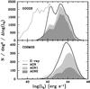 |
Fig. 1 Source density distribution with intrinsic X-ray luminosity distribution for CDFS (upper panel, ~140 arcmin2) and COSMOS (lower panel, 1.8 deg2) samples (note the y-axes are different). The distributions were obtained with a moving bin of width log (LX) = 0.6, with measurements taken each log (LX) = 0.2. The overall X-ray population is represented by the dotted line, the AGN by the solid line. The AGN population is further separated into the type-1 (light shaded region, log (NH [cm-2] ) ≤ 22), type-2 (dark shaded region, log (NH [cm-2] ) > 22), and unknown-type (white region) subpopulations. The regions do not overlap. The unknown-type AGN are those for which data was not enough to allow for an obscuration determination. |
Sample.
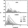 |
Fig. 2 Redshift distribution for CDFS (upper panel) and COSMOS (lower panel) samples (note the y-axes are different). The histograms are cumulative, and no moving bin was applied. Line and region coding as in Fig. 1. |
3. AGN IR-selection criteria
In Paper I, we have presented an efficiency analysis of different colour−colour diagnostics based on X-rays, optical,
mid-IR (MIR), millimetre and radio samples. Three of the tested AGN selection criteria,
proposed in the literature, consider purely IRAC photometry (Lacy et al. 2004, 2007; Stern et al. 2005; Donley
et al. 2012, referred to henceforth as L07, S05, and D12, respectively), while the
two new criteria proposed in Paper I consider Ks+IRAC (KI) and Ks+IRAC+MIPS24 μm (KIM)
photometry. The colour−colour
constraints for KI and KIM are as follows: ![Mathematical equation: \begin{eqnarray} \rm{KI} &\equiv& \begin{cases} K_{\rm s}-\left[4.5\right]>0 \\ \left[4.5\right]-\left[8.0\right]>0 \end{cases} \\ \rm{KIM} &\equiv& \begin{cases} K_{\rm s}-\left[4.5\right]>0 \\ \left[8.0\right]-\left[24\right] > 0.5 \\ \left[8.0\right]-\left[24\right] > -2.9\times(\left[4.5\right]-\left[8.0\right])+2.8. \end{cases} \end{eqnarray}](/articles/aa/full_html/2014/02/aa22267-13/aa22267-13-eq40.png) These
two criteria were developed with the goal of achieving maximum efficiency (select more AGN
sources with less contamination by non-AGN sources) using a minimum number of filters in
order to optimize telescope observing time. They were especially designed for deep fields
and took the JWST wavelength coverage into account. The considered filters – Ks,
4.5 μm,
8.0 μm, and
24 μm (or
2.0 μm,
4.4 μm,
7.7 μm, and
18 μm during
JWST science mission, see Sect. 7) – are believed to
be the key to tackling the photometric degeneracy between AGN sources and high-redshift
dusty starbursts.
These
two criteria were developed with the goal of achieving maximum efficiency (select more AGN
sources with less contamination by non-AGN sources) using a minimum number of filters in
order to optimize telescope observing time. They were especially designed for deep fields
and took the JWST wavelength coverage into account. The considered filters – Ks,
4.5 μm,
8.0 μm, and
24 μm (or
2.0 μm,
4.4 μm,
7.7 μm, and
18 μm during
JWST science mission, see Sect. 7) – are believed to
be the key to tackling the photometric degeneracy between AGN sources and high-redshift
dusty starbursts.
In Paper I, we show that, overall, KI recovers ~50–60% of the total AGN sample (its completeness,
 ),
and ~50–90% of the KI-selected
sample reveals AGN activity at X-rays and/or optical spectral regimes (its reliability,
ℛ). KIM is less complete than
KI, recovering ~30–40% of the
total AGN sample, but equally (or more) reliable with ~75–90% of the KIM-selected sample revealing
AGN activity. The ℛ values
should be regarded as lower limits, given that the X-rays and optical spectral regimes
themselves do not provide a complete sample of AGN sources. This also means that
values should be used for comparison between criteria and not assumed as real values.
),
and ~50–90% of the KI-selected
sample reveals AGN activity at X-rays and/or optical spectral regimes (its reliability,
ℛ). KIM is less complete than
KI, recovering ~30–40% of the
total AGN sample, but equally (or more) reliable with ~75–90% of the KIM-selected sample revealing
AGN activity. The ℛ values
should be regarded as lower limits, given that the X-rays and optical spectral regimes
themselves do not provide a complete sample of AGN sources. This also means that
values should be used for comparison between criteria and not assumed as real values.
Compared to the Lacy et al. (2007, L07), Stern et al. (2005, S05), and Donley et al. (2012, D12) criteria, the most significant improvement by
KI and KIM is achieved at 1 < z ≤ 2.5. At these
redshifts, KI (with  and ℛ = 53 ± 12%5) and KIM (with
  and ℛ = 64 ± 20%) are more
reliable than L07 (ℛ = 29 ± 5%)
and S05 (ℛ = 27 ± 6%), and KI is
more complete than D12 (
and ℛ = 64 ± 20%) are more
reliable than L07 (ℛ = 29 ± 5%)
and S05 (ℛ = 27 ± 6%), and KI is
more complete than D12 ( ).
At z ≲ 1,
although our sample did not allow for a conclusive answer, a larger yet shallower WISE
sample (likely dominated by z ≲ 1 sources) compiled by Assef et al. (2013) has distinguished KI and KIM among the best criteria.
At higher redshifts (z ≳ 2.5, where criteria using <8 μm wavebands fail), KIM
is believed to be the best criteria purely based on a model analysis.
).
At z ≲ 1,
although our sample did not allow for a conclusive answer, a larger yet shallower WISE
sample (likely dominated by z ≲ 1 sources) compiled by Assef et al. (2013) has distinguished KI and KIM among the best criteria.
At higher redshifts (z ≳ 2.5, where criteria using <8 μm wavebands fail), KIM
is believed to be the best criteria purely based on a model analysis.
Overall, L07 is the most complete criteria ( ),
but also the least reliable (ℛ ~ 30−55%), while at the other extreme, D12 is always the most
reliable (ℛ ~ 75−100%,
although affected by low statistical significance), but the least complete
(
),
but also the least reliable (ℛ ~ 30−55%), while at the other extreme, D12 is always the most
reliable (ℛ ~ 75−100%,
although affected by low statistical significance), but the least complete
( ).
S05 selects a comparable number of AGN (
).
S05 selects a comparable number of AGN ( )
to KI, but with less reliability (
)
to KI, but with less reliability ( ).
KI and KIM are thus believed to be the best alternative, with KI more complete, yet
contaminated by z ≳ 2.5 non-AGN sources. This effect is expected not to
affect KIM, making this criterion the best alternative in deep surveys, unless a flux cut is
adopted.
).
KI and KIM are thus believed to be the best alternative, with KI more complete, yet
contaminated by z ≳ 2.5 non-AGN sources. This effect is expected not to
affect KIM, making this criterion the best alternative in deep surveys, unless a flux cut is
adopted.
4. Selection of type-1/2 and low-/high-luminosity sources
The next step in evaluating the AGN IR-criteria is to characterize the selected AGN population in terms of luminosity and obscuration. Previous studies have claimed that IR colour–colour criteria are biased toward unobscured systems (broad-line AGN or type-1 AGN; Stern et al. 2005; Donley et al. 2007; Cardamone et al. 2008; Eckart et al. 2010; Mateos et al. 2013) and tend to select the most luminous objects, missing many low-luminosity ones (Treister et al. 2006; Cardamone et al. 2008; Donley et al. 2008, 2012; Eckart et al. 2010). These tendencies are also assessed in this section.
For the purpose of estimating AGN obscuration, there are many alternatives in the literature, each with its own bias(es). As a result, results will eventually be different in each work. In Appendix A we discuss the bias affecting different approaches depending on survey characteristics and redshift. The analysis presented in Appendix A and in Paper I, and the limitations of the HR method (Eckart et al. 2006; Messias et al. 2010; Brightman & Nandra 2012) justify our choice of adopting a statistically corrected NH estimate (described in Paper I) to assess X-ray obscuration. We believe this is the most reliable approach by allowing for such a large AGN sample throughout a wide redshift range.
Given the occasional small number statistics we are dealing with in this section, we
estimate the statistical error as  ,
where the negative sign refers to the lower error and the positive sign to the upper
error6. Some advantages of this alternative over the
traditional
,
where the negative sign refers to the lower error and the positive sign to the upper
error6. Some advantages of this alternative over the
traditional  is that the upper error does not tend to zero for N → 0, and it retrieves a non-zero lower error for
N = 1. For
large N, both errors tend to the traditional assumption,
.
is that the upper error does not tend to zero for N → 0, and it retrieves a non-zero lower error for
N = 1. For
large N, both errors tend to the traditional assumption,
.
4.1. AGN IR-selection dependency on luminosity
We again emphasize that the aim of IR colour–colour criteria is the selection of galaxies with an IR SED dominated by AGN light. However, low-luminosity AGN will often not dominate the IR emission of a galaxy, making their IR selection unlikely. This is clearly seen in Fig. 3, where the completeness of the L07, S05, and KI AGN selection criteria increases significantly with source luminosity, in agreement with previous work (Treister et al. 2006; Cardamone et al. 2008; Donley et al. 2008; Eckart et al. 2010). If, as indicated by previous work, type-1 AGN tend to be more luminous than type-2 AGN (see the discussions in Treister et al. 2009; Bongiorno et al. 2010; Burlon et al. 2011; Assef et al. 2013, and references therein), this will then lead to a higher fraction of type-1 objects among IR-selected AGN samples. However, it is important to stress that this would not necessarily imply a higher sensitivity of IR criteria toward type-1 AGN, but would mostly be a natural result of luminosity dependence.
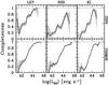 |
Fig. 3 AGN completeness for L07, S05, and KI criteria depending on source X-ray luminosity. The light-grey regions show the associated statistical error. A moving bin is used as described in Fig. 1. |
4.2. Obscuration dependency on luminosity and its evolution with redshift
As just discussed, a possible natural luminosity-obscuration relation may influence the conclusions. In addition, the type-2 fraction has been reported to increase with redshift (Hasinger 2008; Treister et al. 2009; Bongiorno et al. 2010 but see the analysis by Lusso et al. 2013 even though limited to type-1 objects). Here, too, we briefly address these results. Figure 4 shows the variation in the type-2 fraction with intrinsic luminosity, where the fraction presented is A2/(A1 + A2), with A1 and A2 being the numbers of type-1 and type-2 sources, respectively. For improved display of the results, the CDFS and COSMOS samples have been considered together as one (see Appendix A for their separate behaviours). While the top left panel considers the whole AGN sample, the remaining panels consider three redshift intervals with an equal number of AGN: z < 0.89 (top right), 0.89 ≤ z < 1.57 (bottom left), and z ≥ 1.57 (bottom right). The dark-grey shaded regions indicate a crude estimate of the sample completeness for the CDFS and COSMOS X-ray coverage. These are estimated by assuming the intrinsic luminosity of a source at z = 0.89, 1.57, and 3, yielding an observed flux equal to the survey sensitivity. The luminosity range of the regions reflects the column density range 0 ≤ log (NH [cm-2] ) ≤ 24.
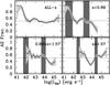 |
Fig. 4 Variation in obscured fraction with source X-ray luminosity in CDFS and COSMOS. The
ratio is A2/(A1 + A2),
where A1 and A2 are the
numbers of type-1 and type-2 sources, respectively. Here, the two samples are
considered together as one. The top left panel considers the whole
AGN sample, while the other panels consider, respectively, z < 0.89 (top
right), 0.89 ≤ z < 1.57
(lower left), and z ≥ 1.57 (lower right) AGN.
A moving bin is used as described in Fig. 1.
Light-grey shaded regions show the associated statistical error, while dark-grey
shaded regions show tentative completeness levels for the CDFS (at low luminosities)
and COSMOS (at high luminosities) samples accounting for column densities of up to
log (NH [cm-2] ) = 24
(see text). The horizontal dotted line shows the overall A2
fraction in each case, |

Overall, we observe a more or less constant type-2 fraction with luminosity at log (LXR [erg s-1] ) ≳ 42 of ~0.5. However, when separating the sample into redshift bins, one observes that luminous AGN (log (LXR [erg s-1] ) ≳ 44) are mostly unobscured up to ~1.6, while the opposite is observed at higher redshifts. A positive increase in the type-2 fraction at these luminosities is also observed if the HR is used instead of NH to assess unobscured/obscured types (see Sect. A) and is in agreement with the literature. Due to sample incompleteness, we do not attempt to measure how the obscuration–luminosity relation evolves with redshift down to lower luminosities. However, based on the evolution at the highest luminosities, we know it has to change, either in its slope or its scaling factor.
4.3. AGN IR-selection dependency on obscuration
Now, assuming the efficiency of IR criteria is clearly dependent on source luminosity, as observed in Fig. 3, the dependency of the type-2 fraction on luminosity (Fig. 4) should dictate the type-2 fraction observed in an AGN sample selected via any AGN IR-criteria. In other words, the IR criteria should present the same type-2 fraction observed in the highest luminosity bins of a given sample. In our case, based on Fig. 4, that would mean a fraction of ~0.5 for IR criteria, but less than 0.5 if a shallower sample (limited to low-redshift sources) would be adopted. Does our sample confirm this pure-luminosity dependence or does it nevertheless imply a bias toward type-1 sources, as defended in the literature?
Figure 5 helps to clarify this point. We recall that
we consider the corrected NH and
 values as
adopted in Paper I. That assumption triggers the trend observed in the top left panel in
Fig. 4 and repeated in Fig. 5 for reference. In Fig. 5, one
observes at least S05 and KI criteria being biased toward type-1 AGN at intermediate
luminosities (43.3 ≲ log (LX [erg s-1] ) ≲ 44),
given that the type-2 fraction for S05- and KI-selected samples is lower than observed for
the whole sample in this luminosity range. At the highest luminosities, the results are
consistent with both types being selected with equal efficiency, since the type-2 fraction
is unchanged. Limiting the study to sources also with reliable photometry in the
MIPS24 band, the
S05 criterion still shows a significant bias toward type-1 AGN.
values as
adopted in Paper I. That assumption triggers the trend observed in the top left panel in
Fig. 4 and repeated in Fig. 5 for reference. In Fig. 5, one
observes at least S05 and KI criteria being biased toward type-1 AGN at intermediate
luminosities (43.3 ≲ log (LX [erg s-1] ) ≲ 44),
given that the type-2 fraction for S05- and KI-selected samples is lower than observed for
the whole sample in this luminosity range. At the highest luminosities, the results are
consistent with both types being selected with equal efficiency, since the type-2 fraction
is unchanged. Limiting the study to sources also with reliable photometry in the
MIPS24 band, the
S05 criterion still shows a significant bias toward type-1 AGN.
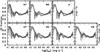 |
Fig. 5 Variation of the obscured fraction (A2/(A1 + A2)) with source intrinsic X-ray luminosity (solid line) for L07 (left), S05 (middle left), KI (middle right), and KIM (right). The top row considers sources with reliable photometry in the Ks + IRAC bands, while the bottom row considers sources with reliable photometry in the Ks + IRAC + MIPS24 bands. The CDFS and COSMOS samples are considered together. The shaded and hatched regions show the associated statistical uncertainty. The dotted line refers to the obscured fraction observed in the whole sample (Fig. 4). A moving bin is used as described in Fig. 1. |
AGN-type selection comparison.
This agrees with the findings of Treister et al. (2009), who noticed a lack of IR excess emission in intermediate-luminosity obscured AGN, even though their analysis is mainly spectroscopically based (which could induce a disagreement with our type-1/type-2 population demography). Also, Mateos et al. (2013), using their IR-selection criterion, show a higher type-1 completeness compared to that observed for type-2 objects at 43 ≲ log (LX [erg s-1] ) ≲ 44, while at higher luminosities the type-2 population is likely to be poorly represented.
To explain this trend, Treister et al. (2009) invoke the effect of self-absorption based on an analysis using Nenkova et al. (2008) clumpy dust-torus models. However, gas may play a role as well. If one considers the scenario where gas is responsible for the bulk of the absorption of X-ray light (see discussion in the following section) or hypothesizes type-2 AGN as having intrinsically higher gas obscuration between the X-ray corona and the dust-torus than type-1 AGN, then one should expect weaker IR emission from type-2 AGN (considering the same amount of circumnuclear dust). Although we are unable to confirm which absorber is dominant in our sample, the gas hypothesis cannot be ruled out as an ingredient to produce this bias toward type-1 AGN. Nevertheless, by basing their analysis mostly on optical spectroscopy, the analysis by Treister et al. (2009) is mostly unaffected by gas absorption (which affects X-rays), thus allowing that dust self-absorption can in principle be behind this type-1-bias in AGN IR-selection.
The general picture of the overall bias observed for each AGN IR-selection criterion is detailed in Table 2. It shows a clear bias towards more X-ray luminous sources and, at a lower level, towards type-1 objects. The latter is more noticeable in S50 and KI criteria. D12, KI, and KIM are the criteria that show the highest high-luminosity fraction (i.e., a higher fraction of high-luminosity AGN).
5. Discussion on AGN IR-selection completeness
In Paper I, overall low completeness (≲50%) was shown for the CDFS sample, especially for the S05, D12, KI, and KIM criteria at z < 2.5. At higher redshifts or brighter flux limits (as in the COSMOS sample), one is restricted to more luminous objects, which are prone to being selected by IR AGN diagnostics (Treister et al. 2006; Cardamone et al. 2008; Donley et al. 2008; Eckart et al. 2010, and Sect. 4.1), resulting in high completeness levels. With decreasing redshifts, however, X-ray observations and optical spectroscopy are able to detect more low-luminosity AGN, sources that will probably not dominate the total IR SED of a galaxy, resulting either from IR-luminous obscured star-formation in the galaxy (Rigopoulou et al. 1999; Veilleux et al. 2009; Nordon et al. 2013) or from the complete absence of a dust torus (e.g., Ho 2008; Asmus et al. 2011; Burlon et al. 2011; Plotkin et al. 2012). The former plays a significant role, since IR-selected AGN have mostly been found in star-forming hosts (Hickox et al. 2009; Griffith & Stern 2010).
But one key reason that affects the completeness at all redshifts is the fact that the major source of obscuration of AGN light is gas. Short time variability for both flux and absorption column density (Elvis et al. 2004; Risaliti et al. 2007; Giustini et al. 2011) implies obscuration material at smaller radii than the dusty torus inner radius, which is set by the sublimation radius (Rsub, e.g., Suganuma et al. 2006; Nenkova et al. 2008). These dust-free gas clouds will only absorb X-ray emission and will not re-emit a continuum spectrum in the IR as dust does. Also, the dusty material, which absorbs UV/optical light, blocks both X-ray and UV/optical emission. X-ray column densities are therefore always higher than those producing the UV/optical obscuration, up to extreme ratios of two orders of magnitude (Maccacaro et al. 1982; Gaskell et al. 2007). These findings imply that dust-free clouds at <Rsub frequently represent the bulk of the X-ray obscuration. As such, the AGN-induced dust emission will be relatively weak or non-existent especially in low-luminosity AGN (Ho 2008; Asmus et al. 2011; Plotkin et al. 2012), but high-luminosity cases also exist where the IR excess is not as extreme as expected (Comastri et al. 2011).
The observed low completeness levels should not be taken as the real completeness levels of AGN IR-selection criteria. At this stage it is impossible to estimate the incompleteness of the X-rays and optical criteria used to assemble our base control sample (Sect. 2). This result just means that, at lower redshifts, there is a population of low-luminosity AGN that will be successfully detected in the X-rays and optical regimes, but completely outshone by the host galaxy light in the IR regime.
6. Strategy for AGN IR-selection
With such a plethora of AGN IR-selection criteria, the astronomer faces a hard decision for which one to adopt. As shown by the many techniques and criteria in the literature, different methods will select either a heterogeneous AGN sample or a subset of it, and with different efficiencies. Based on the results from Paper I and this work, as well as those found in the literature, we propose different strategies depending on survey or sample characteristics to assess the IR AGN population.
If a spectroscopic redshift is available, the astronomer is advised to use:
-
the Ks − [4.5] colour or the Assef et al. (2013) criterion7 at z < 1;
-
the [4.5] − [8.0] colour at 1 < z < 2.5;
-
the [8.0] − [24] at z > 3.
-
the Assef et al. (2013) criterion or the Ks − [4.5] colour aided by a flux cut a la Assef et al. (2013) in samples where only WISE data is available or no deep ≳5 μm data is available;
-
a criterion composed by <8 μm spectral bands in shallow or intermediate-depth coverages, such as L07, S05, D12, or KI, where KI is believed to be the best compromise between completeness and reliability;
-
the KIM criterion for deep coverages or a criterion composed by <8 μm spectral bands aided by a flux cut a la Assef et al. (2013) if no deep 24 μm data is available;
-
extreme optical-to-IR flux ratios (e.g., f24/fR > 1000) in addition to bright flux cuts and/or additional colour cuts (e.g., Fiore et al. 2008; Polletta et al. 2008), in case the goal is to select rare, extremely obscured AGN alone.
7. Adapting KIM to the JWST filter set
Adapting KIM to planned JWST filters is not straightforward. Near-to-mid-IR filters used in
KIM do have different responses from those of JWST. Also, the JWST filter set is richer.
Preferably, the medium-band Ks is replaced by the 2.0 μm broad-band JWST filter,
allowing deeper flux levels to be reached. As for the Spitzer-IRAC
4.5 μm
filter, the JWST 4.4 μm filter is the alternative. As for the
8 μm and
24 μm
filters on board Spitzer, in Paper I, we have proposed the
10 μm and
21 μm
filters as preliminary alternatives. However, using the 10 μm filter creates a
degeneracy between high-redshift AGN and z ~ 1 highly obscured non-AGN starbursts in the
2–8 μm colour
space. Although a morphology analysis could in principle correct this, we now propose
filters 7.7 μm
and 18 μm as
the new alternatives for KIM filters 8 μm and 24 μm (Fig. 6).
Besides preventing the z ~ 1 non-AGN contamination, these two filters are less
affected by the telescope’s thermal emission, thus allowing fainter exposures. The new
colour constraints are the following:
![Mathematical equation: \begin{equation} \rm{KIM_{JWST}} \equiv \begin{cases} \left[2.0\right]-\left[4.4\right]>0 \\ \left[7.7\right]-\left[18\right] > 0.4 \\ \left[7.7\right]-\left[18\right] > -9\times(\left[4.4\right]-\left[7.7\right])+2.2. \end{cases} \end{equation}](/articles/aa/full_html/2014/02/aa22267-13/aa22267-13-eq140.png) (3)The
possible disadvantage is slight contamination by highly obscured non-AGN galaxies at
z > 6. Their existence,
however, is unknown at this stage. Although z > 6 galaxies have been
found already, they show low levels of metallicity (≲Z⊙, Dunlop et al. 2012a, 2013; Zitrin et al. 2012; Jiang et al. 2013), hence low or no dust content. These will appear much bluer in
both [4.4] − [7.7] and
[7.7] − [18] colours.
But the rest-frame UV selection in these works, on the other hand, may be inducing a
selection bias that misses a dust-rich population. For instance, gravitational lensing has
recently revealed two dusty sources at z ~ 5.7 (Vieira et
al. 2013), and large amounts of dust have indeed been found at z > 6, even though only in a QSO
host-galaxy so far (Bertoldi et al. 2003; Gall et al. 2011; Valiante et al. 2011).
(3)The
possible disadvantage is slight contamination by highly obscured non-AGN galaxies at
z > 6. Their existence,
however, is unknown at this stage. Although z > 6 galaxies have been
found already, they show low levels of metallicity (≲Z⊙, Dunlop et al. 2012a, 2013; Zitrin et al. 2012; Jiang et al. 2013), hence low or no dust content. These will appear much bluer in
both [4.4] − [7.7] and
[7.7] − [18] colours.
But the rest-frame UV selection in these works, on the other hand, may be inducing a
selection bias that misses a dust-rich population. For instance, gravitational lensing has
recently revealed two dusty sources at z ~ 5.7 (Vieira et
al. 2013), and large amounts of dust have indeed been found at z > 6, even though only in a QSO
host-galaxy so far (Bertoldi et al. 2003; Gall et al. 2011; Valiante et al. 2011).
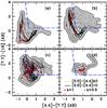 |
Fig. 6 Model colour tracks displayed in the proposed colour−colour space with JWST bands adapted from KIM criterion. Each panel presents a specific group: a) early/late, b) starburst, c) hybrid, and d) AGN. The dotted portion of the tracks refers to the redshift range where [2.0] − [4.4] ≤ 0, and [2.0] − [4.4] > 0 when solid. Red circles and stars along the lines mark z = 1 and z = 2.5, respectively. The light and dark-grey regions show the photometric scatter due to a magnitude error of 0.1 and 0.2, respectively, in the bands considered (equivalent to ~10% and ~20% error in flux, respectively). |
8. Conclusions
This work tests the dependency of AGN selection via IR-colour techniques on source luminosity and obscuration. For that purpose we assembled a deep IR AGN sample in the CDFS and COSMOS fields and characterized it by X-ray luminosity and by obscuration as indicated by X-rays or optical spectroscopy.
We observed the already known strong bias toward high-luminosity AGN and showed that the bias toward type-1 (unobscured) sources is only significant at intermediate luminosities (43.3 ≲ log (LX [erg s-1] ) ≲ 44). At higher luminosities, IR criteria select with equal efficiency type-1 and type-2 AGNe, while at lower luminosities, IR criteria have high incompleteness levels, thus increasing the statistical error dramatically. As a result, AGN IR-selection is genuinely biased toward unobscured AGN, but only at intermediate luminosities. However, we show that type-1 AGN are intrinsically more luminous than type-2 AGN at z ≲ 1.6, thus leading to more type-1 AGN being selected when the IR survey is shallower, as a result of the IR-selection dependency on luminosity (Sect. 4).
We explicitly show the reader that survey characteristics and methods used to assess AGN obscuration do matter. Disregarding this fact will induce large discrepancies when comparing of results (Appendix A).
These results strengthen the strategy where (i) to gather a complete or more reliable AGN sample, one should consider a multi-wavelength set of AGN criteria; (ii) deep X-ray observations are important for recovering the low-luminosity AGNe; and (iii) hard-X-ray observations (such as those with NuSTAR), IR-radio selection, or high-resolution IR imaging (e.g., with JWST) are the key to recovering the (highly-)obscured AGN, especially at low luminosities.
Especially for the AGN IR colour-selection, and considering our study in Paper I and here, as well as work in the literature, we propose a selection strategy that depends on the availability of a reliable redshift measurement, survey depth, or target AGN population (Sect. 6).
Finally, we point out that when JWST comes online, the broad-band filters 2.0 μm, 4.4 μm, 7.7 μm, and 18 μm will be essential for disentangling AGN- from non-AGN-dominated SEDs at depths where spectroscopy becomes impractical, or for AGN selection in case a JWST deep survey is pursued (Sect. 7).
For a more in-depth discussion on the different diagnostics, please consult Donley et al. (2008) and Messias et al. (2012).
When necessary the following relations are used: (K, [3.6], [4.5], [5.8], [8.0])AB = (K, [3.6], [4.5], [5.8], [8.0])Vega + (1.841, 2.79, 3.26, 3.73, 4.40) (Roche et al. 2003, and http://spider.ipac.caltech.edu/staff/gillian/cal.html).
The boundary log (LXR [erg s-1] ) = 43.5 was chosen so that both populations have a reasonable statistical sample.
The lower luminosity limit depends on the obscuration nature of the source, as described in the previous paragraph.
Errors indicated refer to Poisson statistical uncertainty.
This alternative is proposed by the Collider Detector at Fermilab Statistics Committee as described in http://www-cdf.fnal.gov/physics/statistics/notes/pois_eb.txt
W1 − W2 > 0.662 exp { 0.232(W2−13.97)2 }, where W1 and W2 are, respectively, the 3.4 μm and 4.6 μm bands on board WISE.
Acknowledgments
The authors thank the anonymous referee who carefully read the manuscript and helped to improve it. The authors thank the MUSIC, COSMOS, Xue et al. groups for providing public catalogues with essential information, which made the present work possible. H.M. acknowledges the frequent use of Topcat and VOdesk. H.M. acknowledges support from Fundação para a Ciência e a Tecnologia through scholarship SFRH/BD/31338/2006, and from CONICyT-ALMA through a postdoctorate scholarship under project 31100008. H.M. and J.A. acknowledge support from the Fundação para a Ciência e a Tecnologia through projects PTDC/CTE-AST/105287/2008 and PEst-OE/FIS/UI2751/2011. H.M. acknowledges support from UCR while visiting Dr. Bahram Mobasher as a visitor scholar. M.S. acknowledges support from the German Deutsche Forschungsgemeinschaft, DFG Leibniz Prize (FKZ HA 1850/28-1).
References
- Ajello, M., Alexander, D. M., Greiner, J., et al. 2012, ApJ, 749, 21 [NASA ADS] [CrossRef] [Google Scholar]
- Akylas, A., Georgantopoulos, I., Georgakakis, A., Kitsionas, S., & Hatziminaoglou, E. 2006, A&A, 459, 693 [NASA ADS] [CrossRef] [EDP Sciences] [Google Scholar]
- Alonso-Herrero, A., Pérez-González, P. G., Alexander, D. M., et al. 2006, ApJ, 640, 167 [NASA ADS] [CrossRef] [Google Scholar]
- Armus, L., Charmandaris, V., Bernard-Salas, J., et al. 2007, ApJ, 656, 148 [NASA ADS] [CrossRef] [Google Scholar]
- Asmus, D., Gandhi, P., Smette, A., Hönig, S. F., & Duschl, W. J. 2011, A&A, 536, A36 [NASA ADS] [CrossRef] [EDP Sciences] [Google Scholar]
- Assef, R. J., Kochanek, C. S., Brodwin, M., et al. 2010, ApJ, 713, 970 [NASA ADS] [CrossRef] [Google Scholar]
- Assef, R. J., Stern, D., Kochanek, C. S., et al. 2013, ApJ, 772, 26 [NASA ADS] [CrossRef] [Google Scholar]
- Bertoldi, F., Carilli, C. L., Cox, P., et al. 2003, A&A, 406, L55 [NASA ADS] [CrossRef] [EDP Sciences] [Google Scholar]
- Bongiorno, A., Mignoli, M., Zamorani, G., et al. 2010, A&A, 510, A56 [NASA ADS] [CrossRef] [EDP Sciences] [Google Scholar]
- Bower, R. G., Benson, A. J., Malbon, R., et al. 2006, MNRAS, 370, 645 [NASA ADS] [CrossRef] [Google Scholar]
- Brightman, M., & Nandra, K. 2012, MNRAS, 422, 1166 [NASA ADS] [CrossRef] [Google Scholar]
- Brusa, M., Civano, F., Comastri, A., et al. 2010, ApJ, 716, 348 [NASA ADS] [CrossRef] [Google Scholar]
- Burlon, D., Ajello, M., Greiner, J., et al. 2011, ApJ, 728, 58 [NASA ADS] [CrossRef] [Google Scholar]
- Cardamone, C. N., Urry, C. M., Damen, M., et al. 2008, ApJ, 680, 130 [NASA ADS] [CrossRef] [Google Scholar]
- Cardamone, C. N., van Dokkum, P. G., Urry, C. M., et al. 2010, ApJS, 189, 270 [NASA ADS] [CrossRef] [Google Scholar]
- Comastri, A., Fiore, F., Vignali, C., et al. 2001, MNRAS, 327, 781 [NASA ADS] [CrossRef] [Google Scholar]
- Comastri, A., Ranalli, P., Iwasawa, K., et al. 2011, A&A, 526, L9 [NASA ADS] [CrossRef] [EDP Sciences] [Google Scholar]
- Croton, D. J., Springel, V., White, S. D. M., et al. 2006, MNRAS, 365, 11 [NASA ADS] [CrossRef] [Google Scholar]
- Daddi, E., Alexander, D. M., Dickinson, M., et al. 2007, ApJ, 670, 173 [NASA ADS] [CrossRef] [Google Scholar]
- de Grijp, M. H. K., Miley, G. K., Lub, J., & de Jong, T. 1985, Nature, 314, 240 [NASA ADS] [CrossRef] [Google Scholar]
- Dey, A., Soifer, B. T., Desai, V., et al. 2008, ApJ, 677, 943 [NASA ADS] [CrossRef] [Google Scholar]
- Donley, J. L., Rieke, G. H., Rigby, J. R., & Pérez-González, P. G. 2005, ApJ, 634, 169 [NASA ADS] [CrossRef] [Google Scholar]
- Donley, J. L., Rieke, G. H., Pérez-González, P. G., et al. 2007, ApJ, 660, 167 [NASA ADS] [CrossRef] [Google Scholar]
- Donley, J. L., Rieke, G. H., Pérez-González, P. G., et al. 2008, ApJ, 687, 111 [NASA ADS] [CrossRef] [Google Scholar]
- Donley, J. L., Rieke, G. H., Alexander, D. M., Egami, E., & Pérez-González, P. G. 2010, ApJ, 719, 1393 [NASA ADS] [CrossRef] [Google Scholar]
- Donley, J. L., Koekemoer, A. M., Brusa, M., et al. 2012, ApJ, 748, 142 [NASA ADS] [CrossRef] [Google Scholar]
- Draper, A. R., & Ballantyne, D. R. 2009, ApJ, 707, 778 [NASA ADS] [CrossRef] [Google Scholar]
- Dunlop, J. S., McLure, R. J., Robertson, B. E., et al. 2012, MNRAS, 420, 901 [NASA ADS] [CrossRef] [Google Scholar]
- Dunlop, J. S., Rogers, A. B., McLure, R. J., et al. 2013, MNRAS, 432, 3520 [NASA ADS] [CrossRef] [Google Scholar]
- Eckart, M. E., Stern, D., Helfand, D. J., et al. 2006, ApJS, 165, 19 [NASA ADS] [CrossRef] [Google Scholar]
- Eckart, M., McGreer, I. D., Stern, D., Harrison, F. A., & Helfand, D. J. 2010, ApJ, 708, 584 [NASA ADS] [CrossRef] [Google Scholar]
- Edelson, R., & Malkan, M. 2012, ApJ, 751, 52 [NASA ADS] [CrossRef] [Google Scholar]
- Elvis, M., Risaliti, G., Nicastro, F., et al. 2004, ApJ, 615, L25 [NASA ADS] [CrossRef] [Google Scholar]
- Fotopoulou, S., Salvato, M., Hasinger, G., et al. 2012, ApJS, 198, 1 [NASA ADS] [CrossRef] [Google Scholar]
- Fiore, F., Grazian, A., Santini, P., et al. 2008, ApJ, 672, 94 [NASA ADS] [CrossRef] [Google Scholar]
- Fu, H., Yan, L., Scoville, N. Z., et al. 2010, ApJ, 722, 653 [NASA ADS] [CrossRef] [Google Scholar]
- Gall, C., Andersen, A. C., & Hjorth, J. 2011, A&A, 528, A14 [NASA ADS] [CrossRef] [EDP Sciences] [Google Scholar]
- Gaskell, C. M., Klimek, E. S., & Nazarova, L. S. 2007, unpublished [arXiv:0711.1025] [Google Scholar]
- Giacconi, R., Zirm, A., Wang, J., et al. 2002, ApJS, 139, 369 [NASA ADS] [CrossRef] [Google Scholar]
- Gilli, R. 2004, Adv. Space Res., 34, 2470 [Google Scholar]
- Giustini, M., Cappi, M., Chartas, G., et al. 2011, A&A, 536, A49 [NASA ADS] [CrossRef] [EDP Sciences] [Google Scholar]
- Granato, G. L., De Zotti, G., Silva, L., Bressan, A., & Danese, L. 2004, ApJ, 600, 580 [Google Scholar]
- Griffith, R. L., & Stern, D. 2010, AJ, 140, 533 [Google Scholar]
- Hasinger, G. 2008, A&A, 490, 905 [NASA ADS] [CrossRef] [EDP Sciences] [Google Scholar]
- Hatziminaoglou, E., Pérez-Fournon, I., Polletta, M., et al. 2005, AJ, 129, 1198 [NASA ADS] [CrossRef] [Google Scholar]
- Hatziminaoglou, E., Omont, A., Stevens, J. A., et al. 2010, A&A, 518, L33 [NASA ADS] [CrossRef] [EDP Sciences] [Google Scholar]
- Hickox, R. C., Jones, C., Forman, W. R., et al. 2009, ApJ, 696, 891 [Google Scholar]
- Ho, L. C. 2008, ARA&A, 46, 475 [NASA ADS] [CrossRef] [Google Scholar]
- Hönig, S. F., & Kishimoto, M. 2010, A&A, 523, A27 [NASA ADS] [CrossRef] [EDP Sciences] [Google Scholar]
- Hönig, S. F., Kishimoto, M., Gandhi, P., et al. 2010, A&A, 515, A23 [NASA ADS] [CrossRef] [EDP Sciences] [Google Scholar]
- Hony, S., Kemper, F., Woods, P. M., et al. 2011, A&A, 531, A137 [NASA ADS] [CrossRef] [EDP Sciences] [Google Scholar]
- Hopkins, P. F., Hernquist, L., Martini, P., et al. 2005, ApJ, 625, L71 [Google Scholar]
- Hopkins, P. F., Hernquist, L., Cox, T. J., et al. 2006, ApJS, 163, 1 [Google Scholar]
- Hopkins, P. F., Hernquist, L., Cox, T. J., & Kereš, D. 2008, ApJS, 175, 356 [NASA ADS] [CrossRef] [Google Scholar]
- Ilbert, O., Capak, P., Salvato, M., et al. 2009, ApJ, 690, 1236 [NASA ADS] [CrossRef] [Google Scholar]
- Jarrett, T. H., Cohen, M., Masci, F., et al. 2011, ApJ, 735, 112 [NASA ADS] [CrossRef] [Google Scholar]
- Jiang, L., Egami, E., Mechtley, M., et al. 2013, ApJ, 772, 99 [NASA ADS] [CrossRef] [Google Scholar]
- Lacy, M., Storrie-Lombardi, L. J., Sajina, A., et al. 2004, ApJS, 154, 166 [NASA ADS] [CrossRef] [Google Scholar]
- Lacy, M., Petric, A. O., Sajina, A., et al. 2007, AJ, 133, 186 [Google Scholar]
- Laurent, O., Mirabel, I. F., Charmandaris, V., et al. 2000, ApJS, 359, 887 [Google Scholar]
- Lilly, S. J., Le Brun, V., Maier, C., et al. 2009, ApJS, 184, 218 [Google Scholar]
- Lípari, S. L., & Terlevich, R. J. 2006, MNRAS, 368, 1001 [NASA ADS] [CrossRef] [Google Scholar]
- Lipari, S., Terlevich, R., Zheng, W., et al. 2005, Boletín de la Asociación Argentina de Astronomía, 48, 391 [NASA ADS] [Google Scholar]
- Lípari, S., Bergmann, M., Sanchez, S. F., et al. 2009, MNRAS, 398, 658 [NASA ADS] [CrossRef] [Google Scholar]
- Luo, B., Bauer, F. E., Brandt, W. N., et al. 2008, ApJS, 179, 19 [NASA ADS] [CrossRef] [Google Scholar]
- Luo, B., Brandt, W. N., Xue, Y. Q., et al. 2010, ApJS, 187, 560 [NASA ADS] [CrossRef] [Google Scholar]
- Lusso, E., Hennawi, J. F., Comastri, A., et al. 2013, ApJ, 777, 86 [NASA ADS] [CrossRef] [Google Scholar]
- Maccacaro, T., Perola, G. C., & Elvis, M. 1982, ApJ, 257, 47 [NASA ADS] [CrossRef] [Google Scholar]
- Maiolino, R., Gallerani, S., Neri, R., et al. 2012, MNRAS, 425, L66 [NASA ADS] [CrossRef] [Google Scholar]
- Martínez-Sansigre, A., Rawlings, S., Lacy, M., et al. 2005, Nature, 436, 666 [NASA ADS] [CrossRef] [Google Scholar]
- Mateos, S., Alonso-Herrero, A., Carrera, F. J., et al. 2012, MNRAS, 426, 3271 [NASA ADS] [CrossRef] [Google Scholar]
- Mateos, S., Alonso-Herrero, A., Carrera, F. J., et al. 2013, MNRAS, 434, 941 [NASA ADS] [CrossRef] [Google Scholar]
- McCracken, H. J., Capak, P., Salvato, M., et al. 2010, ApJ, 708, 202 [NASA ADS] [CrossRef] [Google Scholar]
- Messias, H., Afonso, J., Hopkins, A., et al. 2010, ApJ, 719, 790 [NASA ADS] [CrossRef] [Google Scholar]
- Messias, H., Afonso, J., Salvato, M., Mobasher, B., & Hopkins, A. M. 2012, ApJ, 754, 120 [NASA ADS] [CrossRef] [Google Scholar]
- Miley, G. K., Neugebauer, G., & Soifer, B. T. 1985, ApJ, 293, L11 [NASA ADS] [CrossRef] [Google Scholar]
- Moretti, A., Vattakunnel, S., Tozzi, P., et al. 2012, A&A, 548, A87 [NASA ADS] [CrossRef] [EDP Sciences] [Google Scholar]
- Nenkova, M., Sirocky, M. M., Ivezić, Ž., & Elitzur, M. 2008, ApJ, 685, 147 [NASA ADS] [CrossRef] [Google Scholar]
- Nordon, R., Lutz, D., Genzel, R., et al. 2013, ApJ, 745, 182 [Google Scholar]
- Petric, A. O., Armus, L., Howell, J., et al. 2011, ApJ, 730, 28 [NASA ADS] [CrossRef] [Google Scholar]
- Plotkin, R. M., Anderson, S. F., Brandt, W. N., et al. 2012, ApJ, 745, L27 [NASA ADS] [CrossRef] [Google Scholar]
- Polletta, M., Weedman, D., Hönig, S., et al. 2008, ApJ, 675, 960 [NASA ADS] [CrossRef] [Google Scholar]
- Richards, G. T., Deo, R. P., Lacy, M., et al. 2009, AJ, 137, 3884 [NASA ADS] [CrossRef] [Google Scholar]
- Rigoloulou, D., Spoon, H. W. W., Genzel, R., et al. 1999, AJ, 118, 2625 [NASA ADS] [CrossRef] [Google Scholar]
- Risaliti, G., Elvis, M., Fabbiano, G., et al. 2007, ApJ, 659, L111 [NASA ADS] [CrossRef] [Google Scholar]
- Roche, N. D., Dunlop, J., & Almaini, O. 2003, MNRAS, 346, 803 [NASA ADS] [CrossRef] [Google Scholar]
- Salvato, M., Hasinger, G., Ilbert, O., et al. 2009, ApJ, 690, 1250 [CrossRef] [Google Scholar]
- Salvato, M., Ilbert, O., Hasinger, G., et al. 2011, ApJ, 742, 61 [NASA ADS] [CrossRef] [Google Scholar]
- Santini, P., Fontana, A., Grazian, A., et al. 2009, A&A, 504, 751 [NASA ADS] [CrossRef] [EDP Sciences] [Google Scholar]
- Scoville, N., Aussel, H., Brusa, M., et al. 2007, ApJS, 172, 1 [NASA ADS] [CrossRef] [Google Scholar]
- Silverman, J. D., Mainieri, V., Salvato, M., et al. 2010, ApJS, 191, 124 [NASA ADS] [CrossRef] [Google Scholar]
- Somerville, R. S., Hopkins, P. F., Cox, T. J., Robertson, B. E., & Hernquist, L. 2008, MNRAS, 391, 481 [NASA ADS] [CrossRef] [Google Scholar]
- Springel, V., Di Matteo, T., & Hernquist, L. 2005, MNRAS, 361, 776 [NASA ADS] [CrossRef] [Google Scholar]
- Stern, D., Eisenhardt, P., Gorjian, V., et al. 2005, ApJ, 631, 163 [NASA ADS] [CrossRef] [Google Scholar]
- Suganuma, M., Yoshii, Y., Kobayashi, Y., et al. 2006, ApJ, 639, 46 [NASA ADS] [CrossRef] [Google Scholar]
- Szokoly, G. P., Bergeron, J., Hasinger, G., et al. 2004, ApJS, 155, 271 [NASA ADS] [CrossRef] [Google Scholar]
- Treister, E., & Urry, C. M. 2005, ApJ, 630, 115 [NASA ADS] [CrossRef] [Google Scholar]
- Treister, E., Urry, C. M., Van Duyne, J., et al. 2006, ApJ, 640, 603 [NASA ADS] [CrossRef] [Google Scholar]
- Treister, E., Virani, S., Gawiser, E., et al. 2009, ApJ, 693, 1713 [NASA ADS] [CrossRef] [Google Scholar]
- Ueda, Y., Akiyama, M., Ohta, K., & Miyaji, T. 2003, ApJ, 598, 886 [NASA ADS] [CrossRef] [Google Scholar]
- Valiante, R., Schneider, R., Salvadori, S., & Bianchi, S. 2011, MNRAS, 416, 1916 [NASA ADS] [CrossRef] [Google Scholar]
- Veilleux, S., Rupke, D. S. N., Kim, D.-C., et al. 2009, ApJS, 182, 628 [NASA ADS] [CrossRef] [Google Scholar]
- Vieira, J. D., Marrone, D. P., Chapman, S. C., et al. 2013, Nature, 495, 344 [NASA ADS] [CrossRef] [Google Scholar]
- Worsley, M. A., Fabian, A. C., Barcons, X., et al. 2004, MNRAS, 352, L28 [NASA ADS] [CrossRef] [Google Scholar]
- Worsley, M. A., Fabian, A. C., Bauer, F. E., et al. 2005, MNRAS, 357, 1281 [NASA ADS] [CrossRef] [Google Scholar]
- Xue, Y. Q., Luo, B., Brandt, W. N., et al. 2011, ApJS, 195, 10 [NASA ADS] [CrossRef] [Google Scholar]
- Zitrin, A., Moustakas, J., Bradley, L., et al. 2012, ApJ, 747, L9 [NASA ADS] [CrossRef] [Google Scholar]
Appendix A: Biases affecting type-1/type-2 demography
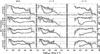 |
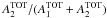
Fig. A.1 Variation in the A2 fraction with source X-ray
luminosity in CDFS (solid line with hatched uncertainty region) and COSMOS (solid
line with shaded uncertainty region). The ratio is A2/(A1 + A2),
where A1 and A2 are the
numbers of type-1 and type-2 sources, respectively. Here, the two samples are
considered individually and at two different redshift ranges (middle and
right columns). The different panels show the effect of different
assumptions while assessing the luminosity and obscuration classes. The
upper two panels show the difference between considering HR or
NH to separate the population into
type-1 (unobscured) and type-2 (obscured) sources. The middle lower panel
shows the effect of adopting the intrinsic luminosity
( |

Besides a possible natural luminosity–obscuration relation and its evolution with redshift (Sects. 4.1 and 4.2), assessing the obscuration level of an AGN is dependent on the technique used for that purpose, thus influencing the final conclusions. Here, we explicitly show the differences.
X-ray obscuration can be assessed via spectroscopic or photometric analysis. While the former is the most reliable, it also limits the analysis to the brightest objects. As a result, the hardness-ratio (HR) or the column density (NH) are estimated photometrically and commonly adopted. The HR is based on photon count ratio (i.e., (H − S)/(H + S), where H and S are the hard- and soft-band counts), which depends on the telescope’s soft-to-hard band relative sensitivity, and is biased towards type-1 objects with increasing redshift (Eckart et al. 2006; Messias et al. 2010). As described in Paper I, NH is estimated based on the soft-to-total flux ratio and redshift, but it requires a correction due to a bias toward type-2 objects with increasing redshift and flux error (Paper I, but see also Akylas et al. 2006; Donley et al. 2012).
In Table A.1, the different approaches are compared while considering the CDFS and COSMOS separately and together. The first row shows the type-2 fractions when HR and the obscured luminosity are adopted. This is the method that retrieves the lowest values. When adopting NH (second row), the increase is significant, especially in COSMOS where it doubles. If one then corrects the observed luminosity to an intrinsic luminosity (third row), the slight differences compared to the second row result from changes in the low-luminosity population (mostly due to the different luminosity lower-limit in the type-1 and type-2 X-ray classification). The bottom row shows the result of correcting the NH estimate, which yields no significant difference in COSMOS, but a significant decrease in CDFS compared to the third row. This is mostly due to the higher fraction of high-redshift sources in the CDFS sample (Fig. 2) for which the NH correction is most relevant.
Assessing the obscured fraction through different methods.
The left column in Fig. A.1 shows how the values reported in Table A.1 depend on luminosity. In CDFS the differences come mostly from discrepancies at log (LXR [erg s-1] ) ≳ 43.6, while in COSMOS it is an overall shift at log (LXR [erg s-1] ) ≳ 42. The middle column shows the same, but only for AGN at z < 1. While the CDFS sample does not show significant differences between methods, the COSMOS samples does show a clear difference between adopting the HR or NH (see the top two panels) at log (LXR [erg s-1] ) ≲ 43.4 (range where COSMOS is likely incomplete, Fig. 4). This can be explained either by the COSMOS survey depth affecting the HR analysis more than the NH analysis of the less luminous objects, or this behaviour is being missed in CDFS given the sample’s higher statistical uncertainty and/or small volume. At the highest redshifts (right column), the COSMOS sample again shows an overall shift to higher type-2 fractions when adopting NH instead of HR, while the CDFS sample shows major differences at log (LXR [erg s-1] ) ≳ 43.6 when statistically correcting the NH method. One possible reason for why one does not observe the same behaviour at these luminosities in the COSMOS sample is that, although both samples are limited to z > 1, the COSMOS statistics are still dominated by the z ~ 1−2 objects (62% of the z > 1 COSMOS sample with log (LXR [erg s-1] ) > 43.6), distances at which the correction is still not considerable. However, the z > 1 CDFS sample has a higher fraction of z > 2 (65% of the z > 1 CDFS sample with log (LXR [erg s-1] ) > 43.6) where the correction starts to be necessary.
Nevertheless, based on the method we have adopted (results shown in the bottom panels), it is interesting to see that within the uncertainties the CDFS trends tend to the values of the COSMOS sample at high luminosities, where the COSMOS survey is expected to be complete.
All Tables
All Figures
|
Fig. 1 Source density distribution with intrinsic X-ray luminosity distribution for CDFS (upper panel, ~140 arcmin2) and COSMOS (lower panel, 1.8 deg2) samples (note the y-axes are different). The distributions were obtained with a moving bin of width log (LX) = 0.6, with measurements taken each log (LX) = 0.2. The overall X-ray population is represented by the dotted line, the AGN by the solid line. The AGN population is further separated into the type-1 (light shaded region, log (NH [cm-2] ) ≤ 22), type-2 (dark shaded region, log (NH [cm-2] ) > 22), and unknown-type (white region) subpopulations. The regions do not overlap. The unknown-type AGN are those for which data was not enough to allow for an obscuration determination. |
| In the text | |
|
Fig. 2 Redshift distribution for CDFS (upper panel) and COSMOS (lower panel) samples (note the y-axes are different). The histograms are cumulative, and no moving bin was applied. Line and region coding as in Fig. 1. |
| In the text | |
|
Fig. 3 AGN completeness for L07, S05, and KI criteria depending on source X-ray luminosity. The light-grey regions show the associated statistical error. A moving bin is used as described in Fig. 1. |
| In the text | |
|
Fig. 4 Variation in obscured fraction with source X-ray luminosity in CDFS and COSMOS. The
ratio is A2/(A1 + A2),
where A1 and A2 are the
numbers of type-1 and type-2 sources, respectively. Here, the two samples are
considered together as one. The top left panel considers the whole
AGN sample, while the other panels consider, respectively, z < 0.89 (top
right), 0.89 ≤ z < 1.57
(lower left), and z ≥ 1.57 (lower right) AGN.
A moving bin is used as described in Fig. 1.
Light-grey shaded regions show the associated statistical error, while dark-grey
shaded regions show tentative completeness levels for the CDFS (at low luminosities)
and COSMOS (at high luminosities) samples accounting for column densities of up to
log (NH [cm-2] ) = 24
(see text). The horizontal dotted line shows the overall A2
fraction in each case, |
| In the text | |
|
Fig. 5 Variation of the obscured fraction (A2/(A1 + A2)) with source intrinsic X-ray luminosity (solid line) for L07 (left), S05 (middle left), KI (middle right), and KIM (right). The top row considers sources with reliable photometry in the Ks + IRAC bands, while the bottom row considers sources with reliable photometry in the Ks + IRAC + MIPS24 bands. The CDFS and COSMOS samples are considered together. The shaded and hatched regions show the associated statistical uncertainty. The dotted line refers to the obscured fraction observed in the whole sample (Fig. 4). A moving bin is used as described in Fig. 1. |
| In the text | |
|
Fig. 6 Model colour tracks displayed in the proposed colour−colour space with JWST bands adapted from KIM criterion. Each panel presents a specific group: a) early/late, b) starburst, c) hybrid, and d) AGN. The dotted portion of the tracks refers to the redshift range where [2.0] − [4.4] ≤ 0, and [2.0] − [4.4] > 0 when solid. Red circles and stars along the lines mark z = 1 and z = 2.5, respectively. The light and dark-grey regions show the photometric scatter due to a magnitude error of 0.1 and 0.2, respectively, in the bands considered (equivalent to ~10% and ~20% error in flux, respectively). |
| In the text | |
|
Fig. A.1 Variation in the A2 fraction with source X-ray
luminosity in CDFS (solid line with hatched uncertainty region) and COSMOS (solid
line with shaded uncertainty region). The ratio is A2/(A1 + A2),
where A1 and A2 are the
numbers of type-1 and type-2 sources, respectively. Here, the two samples are
considered individually and at two different redshift ranges (middle and
right columns). The different panels show the effect of different
assumptions while assessing the luminosity and obscuration classes. The
upper two panels show the difference between considering HR or
NH to separate the population into
type-1 (unobscured) and type-2 (obscured) sources. The middle lower panel
shows the effect of adopting the intrinsic luminosity
( |
| In the text | |
Current usage metrics show cumulative count of Article Views (full-text article views including HTML views, PDF and ePub downloads, according to the available data) and Abstracts Views on Vision4Press platform.
Data correspond to usage on the plateform after 2015. The current usage metrics is available 48-96 hours after online publication and is updated daily on week days.
Initial download of the metrics may take a while.