| Issue |
A&A
Volume 562, February 2014
|
|
|---|---|---|
| Article Number | A107 | |
| Number of page(s) | 10 | |
| Section | Stellar structure and evolution | |
| DOI | https://doi.org/10.1051/0004-6361/201321291 | |
| Published online | 13 February 2014 | |
Spot activity of the RS Canum Venaticorum star σ Geminorum⋆
1 Department of Physics, PO Box 6400014 University of Helsinki, 00014 Helsinki, Finland
e-mail: This email address is being protected from spambots. You need JavaScript enabled to view it.
2 Finnish Centre for Astronomy with ESO (FINCA), University of Turku, Väisäläntie 20, 21500 Piikkiö, Finland
3 Center of Excellence in Information Systems, Tennessee State University, 3500 John A. Merritt Blvd., Box 9501, Nashville, TN 37209, USA
Received: 14 February 2013
Accepted: 6 November 2013
Abstract
Aims. We model the photometry of RS CVn star σ Geminorum to obtain new information on the changes of the surface starspot distribution, that is, activity cycles, differential rotation, and active longitudes.
Methods. We used the previously published continuous period search (CPS) method to analyse V-band differential photometry obtained between the years 1987 and 2010 with the T3 0.4 m Automated Telescope at the Fairborn Observatory. The CPS method divides data into short subsets and then models the light-curves with Fourier-models of variable orders and provides estimates of the mean magnitude, amplitude, period, and light-curve minima. These light-curve parameters are then analysed for signs of activity cycles, differential rotation and active longitudes.
Results. We confirm the presence of two previously found stable active longitudes, synchronised with the orbital period Porb = 19 60, and found eight events where the active longitudes are disrupted. The epochs of the primary light-curve minima rotate with a shorter period Pmin,1 = 1947 than the orbital motion. If the variations in the photometric rotation period were to be caused by differential rotation, this would give a differential rotation coefficient of α ≥ 0.103.
Conclusions. The presence of two slightly different periods of active regions may indicate a superposition of two dynamo modes, one stationary in the orbital frame and the other one propagating in the azimuthal direction. Our estimate of the differential rotation is much higher than previous results. However, simulations show that this may be caused by insufficient sampling in our data.
Key words: stars: activity / starspots / stars: individual: sigma Geminorum
Analysed photometry and numerical results are only available at the CDS via anonymous ftp to cdsarc.u-strasbg.fr (130.79.128.5) or via http://cdsarc.u-strasbg.fr/viz-bin/qcat?J/A+A/562/A107
© ESO, 2014
1. Introduction
The RS CVn-type star σ Geminorum is a bright (V ≈ 4.14), variable binary with a relatively long orbital period  (Duemmler et al. 1997). The primary component is a K1III giant, but the secondary is not visible and has no noticeable effect on the spectrum of the binary. The secondary is most likely a cool, low-mass main-sequence star or possibly a neutron star (Duemmler et al. 1997; Ayres et al. 1984). The inclination of the rotational axis of the primary is roughly 60° (Eker 1986).
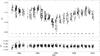 |
Fig. 1 Differential magnitudes between σ Gem and HR 2896, and the check star υ Gem and HR 2896 between the years 1987 and 2010. Different observing seasons are denoted by their corresponding segment number. |
The photometric variability of σ Gem was first detected by Hall et al. (1977). Since 1983, intensive and continuous photometric observations have been made with automated photometric telescopes (APT). The light-curves acquired in this fashion have been studied in detail, for example, by Fried et al. (1983), Henry et al. (1995), Jetsu (1996), and Zhang & Zhang (1999).
Doppler imaging has been used to construct surface temperature maps of σ Gem (Hatzes 1993; Kovári et al. 2001). These surface images had no polar spots, a feature often reported in other active stars. Instead, the spot activity appears to be constrained into a latitude band between 30° and 60°.
In most late-type stars, no unique, regular and persistent activity cycle has been found. In the case of σ Gem, various analyses have yielded a wide range of different possible quasi-periodicities, which are assumed to be an indication of a possible stellar cycle, similar to the 11-year sunspot cycle. Strassmeier et al. (1988) suggested a possible 2.7-year period in the spotted area of σ Gem. Henry et al. (1995), who found a cycle of 8.5 years instead, suggested that the 2.7-year period is related to the lifetime of individual spot regions and hence this shorter period would not represent a true spot cycle. They also attributed the 5.8-year cycle found by Maceroni et al. (1990) to the spot-migration rate determined by Fried et al. (1983).
The light-curve minima of σ Gem have shown remarkable stability in phase over time spans of years or even decades. This indicates a presence of active longitudes, a phenomenon often seen in chromospherically active stars. Active longitudes are longitudinally concentrated areas that show persistent activity, manifesting as starspots. Active longitudes on σ Gem have previously been studied by Jetsu (1996) and Berdyugina & Tuominen (1998). The results indicate that the active longitudes are synchronised with the orbital period, with a preference to the line connecting the binary components. Berdyugina & Tuominen (1998) also suggested that there is a possible 14.9-year activity cycle in the star.
Differential rotation has been studied using photometric spot models and Doppler-imaging techniques. Henry et al. (1995) used spot modelling to determine the migration rate of the starspots and arrived at a value for the differential rotation coefficient. Kovári et al. (2007b) analysed Doppler images, using the local correlation technique (LCT). Their analysis indicated anti-solar differential rotation with α = −0.0022 ± 0.0016. Using a different technique for the same data, they also derived a different value α = −0.022 ± 0.006 (Kovári et al. 2007a).
2. Observations
The observations in this paper are differential photometry in the Johnson V passband obtained at Fairborn Observatory in Arizona using the 0.4 m T3 Automated Photometric Telescope (APT). Each observation is a sequence of measurements that were taken in the following order: K, sky, C, V, C, V, C, V, C, sky, and K, where K is the check star, C is the comparison star and V the program star. The comparison star was HR 2896 and the check star was υ Gem. Until 1992, the precision of the measurements was 0.012 mag. Then a new precision photometer was installed and the precision of the subsequent measurements has been ~ 0.004 − 0.005 mag (Fekel et al. 2005). A thorough description of the APT observing procedures has been given by Henry (1999).
The whole time series consists of 2459 observations and spans from JD 2 447 121.0481 (21 November 1987) to 2 455 311.6556 (25 April 2010). The V − C and K − C differential magnitudes are shown in Fig. 1. The numbers displayed in the upper panel refer to the segment division and correspond to different observing seasons. We decided against including previously published data from other sources. The continuous period search (CPS) method is best suited for temporally continuous data of homogeneous quality, and including temporally sparse data may induce unreliable results. This is also the approach taken in previous studies that used the CPS, such as Lehtinen et al. (2012) and Hackman et al. (2013).
3. Data analysis
Here we give a short introduction to the CPS method and how we used it in the time series analysis of our paper. A complete description of the method can be found in Lehtinen et al. (2011). The CPS method has been developed from the three stage period analysis (TSPA) by Jetsu & Pelt (1999). The CPS uses a sliding window to divide the data into shorter datasets and then determines local models using a variable Kth-order Fourier series: ![Mathematical equation: \begin{equation} \hat{y}(t_i) = \hat{y}\left(t_i,\bar{\beta}\right) = M + \sum_{k\,=\,1}^K{\left[B_k\cos{\left(k2\pi ft_i\right)} + C_k\sin{\left(k2\pi ft_i\right)}\right]}. \label{model} \end{equation}](/articles/aa/full_html/2014/02/aa21291-13/aa21291-13-eq18.png) (1)The optimal model order K used for each dataset is determined by the Bayesian information criterion. The highest modelling order used in this study was K = 2. The possibility of a constant model K = 0 is also considered. In that case, the model is simply the weighted mean of the data points yi = y(ti) in the dataset.
(1)The optimal model order K used for each dataset is determined by the Bayesian information criterion. The highest modelling order used in this study was K = 2. The possibility of a constant model K = 0 is also considered. In that case, the model is simply the weighted mean of the data points yi = y(ti) in the dataset.
The first step of the CPS-analysis is to divide the data into datasets. The datasets are composed using a rectangular window function with a predetermined length ΔTmax that is moved forward through the data one night at a time. A new dataset is created each time when the dataset candidate determined by the window function includes at least one new data point that was not included in the previous dataset. Each modelled dataset must also include at least nmin data points to be valid. We used values nmin = 14 and which is roughly two and half times the average photometric period.
The first dataset with a reliable model is called an independent dataset. The next independent datasets are selected with the following two criteria. Firstly, this next independent dataset must not share any common data with the previous independent dataset. Secondly, the model for this next independent dataset needs to be reliable. In other words, these independent datasets do not overlap and their models are always reliable. With this definition, the correlations between the model parameters of independent datasets represent real physical correlations, that is, these correlations are not due to bias caused by common data.
The datasets are combined into segments, each representing a different observing season. The segment division does not directly affect the analysis because each dataset is still analysed separately. The segment division of this analysis is given in Table 1. For each segment, the length of the segment is given, along with the total number of data points, the number of datasets, and the number of independent datasets.
Segments of the σ Gem photometry.
The parameters obtained from the light-curve model as a function of the mean epoch of the dataset, τ, are
-
M(τ) =mean magnitude
-
A(τ) =peak-to-peak light-curve amplitude
-
P(τ) =photometric period
-
tmin,1(τ) =epoch of the primary minimum
-
tmin,2(τ) =epoch of the secondary minimum
-
TC(τ) =time scale of change.
The CPS also provides a graphical representation of the results for each segment. An example of this is given below in Fig.6. That figure contains the following panels:
-
(a)
standard deviation of residuals σ(τ);
-
(b)
modelling order K(τ) (squares, units on the left y-axis); and numberof observations per dataset n (crosses, units on the right y-axis);
-
(c)
mean differential V-magnitude M(τ);
-
(d)
time scale of change TC(τ)
-
amplitude A(τ);
-
(f)
period P(τ);
-
(g)
primary (squares) and secondary (triangles) minimum phases φmin,1(τ) and φmin,2(τ);
-
(h)
M(τ) versus P(τ);
-
(i)
A(τ) versus P(τ);
-
(j)
M(τ) versus A(τ);
Reliable models are denoted with closed symbols and unreliable models with open symbols.
The numerical results of the CPS analysis can be accessed electronically at the CDS. The light-curves and the best-fit models of the independent datasets are shown in Fig. 2. The light-curves are plotted as a function of phase  . For each dataset, the phases φi were first calculated using the best-fit periods P(τ) and the epochs of the primary minima tmin,1(τ). The phases of each dataset were then adjusted by φ′ = φorb,1 − 0.2, where φorb,1 are the phases of the primary minimum epochs tmin,1 of each dataset, calculated using the orbital ephemeris
  . This adjustment was made to ensure that the phases of the primary minima are the same as in Fig. 4. A similar procedure was employed in Lehtinen et al. (2011).
Some of the light-curves in segments 2, 9, and 17 clearly show that the brightness of the star can change during two successive rotations. This could have partly been avoided by using a shorter window. We also analysed the data using a window  , but the result was a large number of unreliable models, therefore we used the longer window
  in the final analysis.
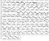 |
Fig. 2 light-curves and best-fit models of independent datasets. The procedure used to calculate the phases is explained at the end of Sect. 3. |
4. Results
4.1. Long-term variability and activity cycles
The photometry of σ Gem has been studied before with intention of searching for long-term activity cycles, but so far, none of the findings has been conclusive. We applied the CPS to the M, A and P estimates of independent datasets, using a first-order model (K = 1). The long-term changes of these parameters are shown in Fig. 3. For the mean magnitudes M, we found the best period to be PM = 6.69 ± 0.21 yr. For A the best period was PA = 3.12 ± 0.25 yr and for P, the best period was PP = 4.4 ± 1.0 yr.
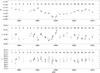 |
Fig. 3 Long-term changes of mean (M), amplitude (A), and period (P). The segment numbers are shown above the data. |
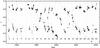 |
Fig. 4 Phases of the light-curve minima of Sigma Geminorum in the orbital frame of reference. Phase φ = 0.8 coincides with the conjunction of the binary components, with the primary in front. The primary and secondary minima of independent datasets are denoted by black squares and triangles, respectively, grey squares and triangles are used for non-independent minima. The line is plotted using an ephemeris of |

We also checked the parameters A, M and P from independent datasets for correlations. One might expect a correlation between the mean brightness and starspot amplitude, simply because when larger parts of the star are covered by starspots, the star should appear dimmer. The starspot amplitude and period might also correlate; with changing latitude the effective covered area seen by the observer changes and due to differential rotation, if present, the period might also change.
Because the dependencies between these parameters are not necessarily linear, we calculated the Spearman rank correlation coefficient and the corresponding p value for each pair of parameters. Unsurprisingly, we found the strongest correlation between M and A, with a correlation coefficient ρ = 0.33 and a p value p = 0.004. For M and P we derived ρ = −0.07 and p = 0.58, and for P and A, ρ = −0.18 and p = 0.13, none of which is statistically significant. Although there is a relatively strong correlation between A and M, the periods PA and PM are different. This is at least partly explained by sometimes more axisymmetric spot coverage, like in the Doppler images by Kovári et al. (2001). In the light-curves obtained during similar spot configurations, the peak-to-peak amplitude of the light-curve can be low, even though the star would appear to be faint.
4.2. Differential rotation
To estimate the stellar differential rotation, starspots have been used as markers that are assumed to rotate across the visible stellar disc with varying angular velocities that are determined by their respective latitudes. To estimate the amount of surface differential rotation present in the star, we used the dimensionless parameter  (2)where Pw ± ΔPw is the weighted average of periods from the independent datasets Pi, given by PW = (ΣwiPi)/ΣPi,
  , and
, and  (Jetsu 1993). The parameter Z gives the ± 3ΔPw upper limit for the variation of the photometric period Pphot.
Using only the period estimates from the independent datasets, we derived the weighted mean of the photometric period  , which gives Z = 0.103. Our amplitude-to-noise ratio for the typical light-curve amplitude A(τ) = 0.10 mag was about 100. This means that spurious changes of Z caused by noise were not significant (Lehtinen et al. 2011, Table 2).
We can use the parameter Z to derive the differential rotation profile of a star (assuming solar-like differential rotation), 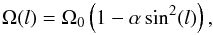 (3)where l is the latitude, Ω0 is the rotation rate at the equator, and α the differential rotation coefficient. The value of α can be estimated with the relation | α | ≈ Z/h (Jetsu et al. 2000), where h = sin2(lmax) − sin2(lmin), and the parameters lmin and lmax are the lowest and highest latitudes between which the spot activity is confined.
Doppler-imaging results by Hatzes (1993) and Kovári et al. (2001) indicate that most of the spot activity on σ Gem is constrained to latitudes between 30° and 60°, with some activity on lower latitudes, ± 30° from the equator. This would give values 0.5 ≲ h ≲ 0.75, yielding an α in the range 0.14 ≲ α ≲ 0.21, or in terms of rotational shear, 0.05 rad d-1 ≲ ΔΩ ≲ 0.07 rad d-1. For comparison, we have listed the previously derived values of the differential rotation coefficient α together with our estimate in Table 2.
Strength of the differential rotation according to different papers.
It is also of interest how the amount of differential rotation relates to other stellar parameters in spotted stars. Henry et al. (1995) reported a relation for the rotation period and the differential rotation. In comparison to their result, even our quite high estimate for the differential rotation is in the expected range for this photometric period. Collier Cameron (2007) provided a relation between the effective temperature of the star and differential rotation rate ΔΩ,  (4)where Teff is the effective temperature of the star in Kelvin and ΔΩ is given as radians per day. Using the effective temperature Teff = 4630 K from Kovári et al. (2001), we derive ΔΩ ≈ 0.022. This is clearly lower than our estimate for the differential rotation rate. On the other hand, we also note that some of the differential rotation estimates for similar stars, which were used to derive the above relation, have values similar to our estimate.
To estimate the reliability of our result, we calculated synthetic photometry using the spot-model by Budding (1977). We used a two-spot model without differential rotation, that is, the spots rotated with a constant period P = Porb. We sampled the synthetic light-curve at the same observation times as in the original data and added normally distributed noise with zero mean and standard deviation σN = 0.007, calculated from the standard deviation of the residuals ϵ = y(ti) − ŷ(ti) of our CPS model. The spot model parameters were calculated to correspond to the location of the active longitudes and the spot-modelling results from Kovári et al. (2001) as closely as possible. For the spot latitudes λi, longitudes βi and radii ri we used values λ1 = 108°, λ2 = 284°, r1 = 25°, r2 = 25°, β1 = 20°, and β2 = 10°.
For the inclination of the star, we used the value i = 60°. The values we used for the linear limb-darkening coefficient u and spot-darkening fraction κ were u = 0.79 and κ = 0.57. The spot-darkening fraction corresponds to a temperature difference between the photosphere Tphot = 4630 K and a cool spot Tspot = 4030 K. The linear limb-darkening coefficient for the Johnson V-band was calculated using the results by Claret (2000) and bilinear interpolation. The parameters used were T = Tphot, log g = 2.5, microturbulence vmicro = 1.0 km s-1, and solar metallicity. All these parameters are the same as used in Kovári et al. (2001).
Analysing this synthetic photometry, we derived Zsynth = 0.033. This result clearly demonstrates that our differential rotation estimate is affected by the long rotation period combined with poor sampling. More complex models, such one with an added third spot, rotating with a period of  , did not change this result, neither did adding artificial ff-events.
4.3. Active longitudes
Active longitudes are longitudes on the surface of a star that exhibit persistent spot activity. They can appear in pairs, situated on the opposite sides of the star (Henry et al. 1995; Jetsu 1996; Berdyugina & Tuominen 1998). The presence of active longitudes in observational data is well established in many active stars and they are thought to be manifestations of non-axisymmetric dynamo modes. σ Gem has shown very persistent active longitudes throughout its whole observational history (Jetsu 1996). Moreover, the active longitudes on σ Gem are synchronised with the orbital period of the tidally locked binary components, whereas on many other RS CVn stars, the active longitudes have been reported to migrate linearly in relation to the orbital reference frame (e.g., Berdyugina & Tuominen 1998; Lindborg et al. 2011).
The phase diagram of the light-curve minima tmin,1 and tmin,2 (Fig. 4) clearly shows the two active longitudes that are, with a few exceptions, present throughout the whole time series. The phases φorb were calculated with the orbital period, using the ephemeris (Duemmler et al. 1997), and were then adjusted for plotting using the formula φ = φorb − 0.2. Thus, phase φ = 0.8 marks the conjunction of the two binary components, with the primary in front.
The epochs of the light-curve minima from independent datasets, tmin,1 and tmin,2, were simultaneously analysed using the non-weighted Kuiper-test. The Kuiper-test is a non-parametric test that is suited for searching for periodicity in a series of time points ti, when the phases, calculated using period P,  have a bimodal (or even multimodal) distribution. We used the same formulation as in Jetsu (1996). We used a null hypothesis (H0), that the phases φP,i are uniformly distributed within the interval [0,1], that is, there is no periodicity present. The period search was made within the interval 0.85PW < P < 1.15PW, where PW is the weighted average of the photometric periods. The resulting best period was
  and the corresponding critical level was Q = 8.52 × 10⁻⁶.
Figure 4 shows that during segments 8−13 and 15−19 the primary minima are rotating faster than the orbital period of the binary system. Therefore, we also analysed only the independent primary minima tmin,1 using the Kuiper-test and obtained the best period  with Q = 1.05 × 10⁻⁶.
If the drift of the primary minima were present only during single segments, this effect could be introduced by an evolving spot pattern or differential rotation. However, the primary minima trace a clearly identifiable path that can be seen for many years. The aforementioned effects would only apply to single spots, not whole active areas such as active longitudes.
The main contribution to Pmin,1 comes from segments SEG9, SEG14, and SEG17. During these segments the secondary minima vanish altogether and the primary minimum is shifted ~0.25 in phase. As a result, these segments with only one minima throughout the whole segment are also the only ones that are not situated near the active longitudes. This could be caused two relatively close starspots that form a single minimum, in between their respective longitudes, or by a temporary disturbance of the usual spot configuration (where spots are located near active longitudes) by additional new starspots.
Emergence of additional star spots could also be explained with an azimuthal dynamo wave moving across the star (Krause & Raedler 1980; Cole et al. 2013). This possibility is even more interesting, because it appears that the intermittent disappearance of the stable active longitudes is somehow connected to the jump of activity between the two active longitudes; during several occasions, the primary and secondary minima switch places when the migrating primary minimum reaches either of the active longitudes. The diagonal dashed line in Fig. 4 shows the movement of the primary minima. The line is plotted using an ephemeris of  .
.
4.4. Flip-flops and flip-flop-like events
Flip-flops are a name coined by Jetsu et al. (1993) in their analysis of the active giant FK Com photometry. A flip-flop is an event where the primary and secondary minima suddenly switch their places in a phase diagram. We refer to these types of events as ff-events. An obvious interpretation is that during an ff-event, the activity jumps from one active longitude to another.
In the σ Gem data, several jumps in the phase diagram can be seen. Since all of these flip-flop candidates are not necessarily similar, physically related phenomena, we used the following criteria to distinguish true ff-events from false ones:
-
CI:
The region of main activity shifts by about 180 degrees from theold active longitude and then remains on the new active longitude.
and
-
CII:
The primary and secondary minima are first separated by about180 degrees. Then the secondary minimum evolves into alonglived primary minimum, and vice versa.
Although multiple phase shifts can be found in the data, there is only one activity shift, between segments one and two, that fulfils these two criteria. In addition, there are multiple events similar to ff-events that are abrupt, but not persistent, or are associated with gradual migration of the primary minima that take years to complete. These events are called ab-events and gr-events, respectively.
4.4.1. Flip-flop event 1988–1989
The only ff-event in the data that fulfils our criteria CI and CII occurs between segments SEG1 and SEG2 and has been identified in previous papers that used contemporaneous data, that is, Jetsu (1996) and Berdyugina & Tuominen (1998). The first signs of an approaching ff-event can be seen at the end of SEG1, where the light-curve shows a gradual deepening of the secondary minimum. The switch could have occurred even before the end of SEG1; in the last few models of the segment, the minima have already switched places, but the models are not reliable due to the small number of observations. At the beginning of SEG2, the previous secondary minimum has become the new primary minimum. After the ff-event, the primary and secondary minimum remain stable for several years.
4.4.2. Gradual events
Signs of an approaching phase shift can be seen already at the end of SEG8. In this case, however, the phase shift is gradual and caused by a weakening of the primary minimum, instead of by deepening of the secondary, that is, the activity does not “jump” from an active longitude to another, but diminishes on one and remains constant on the other. During this segment, the star is at its brightest, and correspondingly, the light-curve amplitude is very low, decreasing throughout segments SEG8–SEG10.
During SEG9 the secondary minimum vanishes altogether, giving way to a relatively unstable primary, situated halfway between the previous two active longitudes.
As seen in the light-curves (Fig. 2), the new minimum is also extremely wide, most likely consisting of several large starspots. The minimum persists until the beginning of SEG10. There are several unreliable datasets in the beginning of this segment, during which two separate minima emerge from the previous single minimum. This type of phase diagram is expected when two close starspots rotate with different periods, gradually moving away from each other (Lehtinen et al. 2011, Fig. 3).
The Doppler images by Kovári et al. (2001) taken between 1 November 1996−9 January 1997, and overlapping with the first part of segment 10, show three large starspots distributed almost at equal distances in longitude on a latitude band situated between 0° and 60°. The photometric spot models in the same paper also show three spots (Spots 1−3), of which spots 1 and 2 correspond to the persistent active longitudes. This view does not support the idea that the two large spots rotate at different rates.
We consider it to be more likely that the previously almost band-like spot distribution is vanishing or that the third spot (Spot 3) slowly migrates and merges with the other active longitude (Spot 1). In our analysis, the beginning of SEG10 shows two minima, with the primary minima linearly migrating from φ = 0.5 towards the other active longitude at φ = 0.3. This supports the idea that the first and third spot merge. After this, the stable active longitudes again start to dominate the light-curve, only this time, the primary and secondary minima have switched places.
During 2000−2002 and 2003−2005, the star again shows similar behaviour. During SEG13 the two active longitudes are present, but they disappear in SEG14 and are replaced by a single minimum, located halfway between the active longitudes. In SEG15, the two active longitudes are present again, and the minima have switched their places.
In SEG17 the active longitudes disappear once again and are recovered in the following segment, now with switched primary and secondary minima. In contrast to the 1996−1997 event, the amplitude of the light-curve and the mean brightness of the star do not show any changes or patterns during the time span between 2000 and 2005. There is a weak linearly growing trend in the mean brightness, but it does not correlate in any way with amplitude or period during that time.
4.4.3. Multiple ab-events between 2005 and 2010
The area of main activity jumps multiple times from one active longitude to another during the last five years of the time series. Unlike before, these phase shifts happen in brief succession, with intervals of only about a year or two. The first ab-event, during SEG19, can be seen in the light-curves and persists until the following SEG20, where the primary minimum switches back. In SEG20 and SEG21 the same happens again: the activity jumps from one active longitude to another and back again in relatively short time. Although the phase shifts are not persistent, the primary minima are quite deep in each case and the shifts are most likely real and not just random fluctuation or observational errors.
4.5. Flip-flop event cycles
We determined epochs for each ff-, ab-, and gr-event. In the case of ff- and ab-events, we used the mean epoch of the two primary minima between which the phase shift occurred. For gr-events, we determined the epoch from the moment when the primary minimum reached and remained on the active longitude in question. Jetsu (1996) determined the width of the active longitudes to be 0.2 in phase, therefore we required that the primary minimum satisfied inequality | φmin,1 − φal,i | < 0.1, where φal,i is the mean phase of an active longitude.
The mean phases of the two active longitudes were calculated from independent datasets so that each minimum contributed only to the mean of the active longitude it is closest to in phase, and only datasets with two minima were used. The phases we derive for the two active longitudes are φal,1 = 0.79 and φal,2 = 0.30.
The events are tabulated in Table 3. There is also one earlier flip-flop, found by Jetsu (1996) and later confirmed by Berdyugina & Tuominen (1998). The epoch of the flip-flop is taken from the latter publication.
To investigate the possibility that an azimuthal dynamo wave could be responsible for the ff- and gr-events, we analysed their respective epochs using the Kuiper-test with the period interval Pmin = 2.0 yr and Pmax = 10.0 yr. We found the best period Pff,1 = 2.67 yr,Vn = 0.81. We consider the second best period Pff,2 = 7.99 yr, Vn = 0.74 to be more plausible, however, partly because the shorter period would imply that there are multiple unobserved flip-flop epochs, and partly because the 2.67-year period is an integer part of the 7.99-year period. The periodogram is plotted in Fig. 5. The small number of time points makes it impossible to calculate meaningful significance estimates for the Kuiper-test statistics Vn; for this, more events would be required.
Ff-, gr-, and ab-events found in the data.
5. Discussion
5.1. Differential rotation
The value we derive for differential rotation is an order of a magnitude higher than the values found in previous studies. The main culprit is most likely the long rotation period. In some cases, this leads to poor phase coverage which, in turn leads to large uncertainties in the period estimates. Another problem the long rotation period causes is the possibility that the spot structure changes on the surface of the star. In the phase diagrams of some datasets this can be seen as a superposition of two light-curves with noticeably different shapes. In a worst-case scenario these two effects appear simultaneously, that is, the spot structure changes between successive rotations, but this is not noticeable because of the poor phase coverage. Thus the phase diagram can create an illusion of a unique, continuous light-curve, while in fact it was created by two different spot configurations, introducing an error to the period estimate.
Henry et al. (1995) used some of the same data analysed in this paper. The discrepancy between our and their differential rotation estimates can be easily attributed to the different approaches that were used. Henry et al. (1995) used spot modelling, and the differential rotation estimate was derived from the longest and shortest periods determined from the spot migration curve of each spot.
In our analysis even slight changes in the spot structure, occurring faster than the rotational period, could lead to a change in the period estimate, which we then interpret as differential rotation. In Lehtinen et al. (2011), only the signal-to-amplitude ratio was considered when the amount of spurious period change was estimated. Our simulated data indicated that the sampling effects are also a considerable source of spurious period changes and can result in overestimates of the differential rotation.
When comparisons are made to other stars with a similar period, the range of differential rotation these stars exhibit is larger than the difference between measurement techniques. There is also considerable doubt whether starspots are even reliable proxies of differential rotation. Even spots on the same latitude might have different migration rates due to different anchor depths. This is shown by recent numerical simulations, which indicate that if observed starspots are caused by a large-scale dynamo field, their movement is not necessarily tracing the surface differential rotation, but the movement of the magnetic field itself (Korhonen & Elstner 2011). Finally, observed spots are not necessarily even stable or may consist of many small rapidly evolving starspots instead of one large spot. In any case, it is clear that the use of the CPS method might greatly overestimate differential rotation, if the rotation period is long.
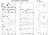 |
Fig. 6 CPS-analysis of segment SEG3. The contents of the panels are explained at the end of Sect. 3. |
5.2. Active longitudes and flip-flop events
We found three types of events in which the activity moves from an active longitude to another. In addition to the single flip-flop fulfilling the criteria CI and CII (ff-events), we found ab-events and gr-events. It is not clear whether or not these different types of events are caused by the same phenomenon or not. A similar type of two-fold behaviour of ab- and gr-events has been reported in FK Com, by Oláh et al. (2006) and Hackman et al. (2013), for instance.
The ab-events are similar to the flip-flops discovered by Jetsu et al. (1993): sudden shifts of primary minima from one active longitude to another. The only difference is that the phase-shift is not persistent inab-events and the area of the main active region shifts back to the original active longitude after about a year. Unfortunately, it is almost impossible to determine which ab-events are fundamentally different from “real” ff-events, that is, sudden, but persistent phase shifts. Some of the ab-events could fail to fulfil the criteria for ff-events simply because the event is followed by an unrelated ab-event, which would create an appearance of a non-persistent phase-shift.
During the gr-events, the location of the main active region shifts by ~90° in longitude and the photometry shows only one wide minimum. The disappearance of the two long-lived active longitudes and their replacement with only one minimum could be illusory at least in SEG9. The overlapping Doppler images dated to the beginning of SEG10 show that there is a large spot area near the longitude the single minimum was located at.
The appearance of spots between the active longitudes resembles what Oláh et al. (2006) found in photometry of FK Com and called phase-jumps. In a phase-jump, old active areas disappear and then new ones emerge, with an offset of roughly 90° with respect to the original active longitudes. In FK Com, the phase jumps cause the active longitudes to stay displaced for a much longer time (Hackman et al. 2013). It could be that the binary nature of σ Gem affects the preferred location of the active longitudes and this displacement is not long-lasting.
In segments SEG10, SEG14, SEG17, and SEG18 the primary minimum traces a path towards the active longitude situated at φal,2 = 0.3. This may imply that in addition to the stable non-axisymmetric dynamo mode, there is also a possible azimuthal dynamo wave present, rotating faster than the star itself. This is also suggested by the period of the primary minima, which is shorter than the orbital period of the tidally locked binary system.
If present and rotating at a constant rate, the wave would return to a same active longitude every 7.9 years. This period is remarkably close to the 7.99-year period we found from the epochs of the gr- and ff-events. It is possible that at least some of these observed events occur when a spot structure corresponding to a moving dynamo wave interferes with the stable active longitudes, either strengthening or weakening the minima as it passes by. This does not prevent the ab-events from also being caused by this mechanism. In this model, the time between successive flip-flops is equal only when the apparent spot coverage on both of the active longitudes is equal. If the spot coverage on either of the active longitudes is greater, the primary minimum will remain on this active longitude for a longer time. To further complicate things, the spot coverage on the active longitudes may also change independently of the migrating active area, which can prevent the observation of the gr-events.
If there is an active region migrating in the frame of the orbital period, we should see periodic variation in A. The interference between the stationary active longitudes and the migrating region should modulate the light-curve with an amplitude envelope with the same period as the flip-flop event cycle. We detect no clear sign of such modulation, although events 3 and 4 in Table 3 are associated with relatively low values of A.
It is possible that this amplitude effect is masked by short-term spot evolution. This seems plausible, since the variation in A between independent datasets within one segment is quite strong. Intriguingly, there are also disturbances in the light-curves at multiple occasions, at the same epochs when the presumed dynamo wave passes an active longitude. An example of this can be seen in SEG3 (Fig. 6), where these abrupt changes in the light-curve even prevent reliable CPS modelling. Similar behaviour can be seen in segments SEG11 and SEG19. As for the other CPS-parameters, M and P, there seems to be no obvious connection between them and the ff-, gr-, and ab-events. The periods found from these parameters are also different from the Kuiper-test periods. On the other hand, one may speculate that the 2.67- and 8.5-year periods found by Strassmeier et al. (1988) and Henry et al. (1995), respectively, are somehow connected to the 2.7- and 8.5-year Kuiper-test periods. If either of these periods is real and caused by a migrating spot area, this could very well be reflected in the mean brightness of the star.
6. Summary and conclusions
By applying the CPS method to photometry of σ Gem we have been able to study in detail the long-term evolution of the mean brightness (M), light-curve amplitude (A), and photometric minima (tmin,1,tmin,2) and photometric rotation period (P) of the star. The best periodicities in M, A and P were PM = 6.69 ± 0.21 yr, PA = 3.12 ± 0.25 yr, and PP = 4.4 ± 1.0 yr. Variations in P could be explained by differential rotation, for which we estimated a coefficient of 0.14 ≲ α ≲ 0.21. From the combined time point series of both the primary and secondary minima, we found a period of . When only primary minima were analysed, we retrieved a period . Furthermore, we analysed flip-flops and other gradual and abrupt phase-shift events and found that the best period for these would be 7.99 years. However, the small amount of events prevented a meaningful significance estimate of this period.
There appears to be no direct connection between the periods found from A, M, and P. The only obvious connection between P and the other model parameters could be caused by differential rotation. The differential rotation estimate we derived from the period changes is extremely large when compared to previous analyses (Kovári et al. 2007a,b). Using synthetic photometry, we demonstrated that this is at least partly due to the long rotation period of the star, which sometimes leads to sparse and uneven phase coverage. This can cause strong fluctuations in the period estimates, and thus, an unreasonably high differential rotation estimate.
We also confirmed the presence of previously found persistent active longitudes, which are tied to the orbital reference frame of the binary system. The most interesting result we presented in this paper is the possible connection between the flip-flop-like events and the drift of the primary minima. This may imply that there is a superposition of two dynamo modes operating in the star. One would be tied to the orbital period of the binary system, while the other one could manifest itself as an azimuthal dynamo wave, rotating faster than the star. Signs of such dynamo waves have been observed in other stars (Lindborg et al. 2011; Hackman et al. 2011, 2013, e.g.) and have also been reproduced in numerical MHD-simulations (Cole et al. 2013).
Such an azimuthal dynamo could disturb the stable active longitudes present in the star, creating the ff-, gr-, and ab-events. To find supporting evidence for the presence of a propagating dynamo wave, it would be necessary to obtain new Doppler images of the star, preferably at least two sets taken at different times, and determine, whether or not there are star spots in areas indicated by the ephemeris  .
.
Acknowledgments
This work has made use of the SIMBAD data base at CDS, Strasbourg, France and NASAs Astrophysics Data System (ADS) bibliographic services. The work by P.K. and J.L. was supported by the Vilho, Yrjö and Kalle Väisälä Foundation. The work of T.H. was financed by the project “Active stars” at the University of Helsinki. The automated astronomy program at Tennessee State University has been supported by NASA, NSF, TSU, and the State of Tennessee through the Centers of Excellence program. We thank the referee for valuable comments on the manuscripts.
References
- Ayres, T. R., Simon, T., & Linsky, J. L. 1984, ApJ, 279, 197 [NASA ADS] [CrossRef] [Google Scholar]
- Berdyugina, S. V., & Tuominen, I. 1998, A&A, 336, L25 [NASA ADS] [Google Scholar]
- Budding, E. 1977, Ap&SS, 48, 207 [NASA ADS] [CrossRef] [Google Scholar]
- Claret, A. 2000, A&A, 363, 1081 [NASA ADS] [Google Scholar]
- Cole, E., Käpylä, P. J., Mantere, M. J., & Brandenburg, A. 2013, ApJ, 780, L22 [Google Scholar]
- Collier Cameron, A. 2007, Astron. Nachr., 328, 1030 [NASA ADS] [CrossRef] [Google Scholar]
- Duemmler, R., Ilyin, I. V., & Tuominen, I. 1997, A&AS, 123, 209 [NASA ADS] [CrossRef] [EDP Sciences] [Google Scholar]
- Eker, Z. 1986, MNRAS, 221, 947 [NASA ADS] [Google Scholar]
- Fekel, F. C., Henry, G. W., & Lewis, C. 2005, AJ, 130, 794 [NASA ADS] [CrossRef] [Google Scholar]
- Fried, R. E., Vaucher, C. A., Hopkins, J. L., et al. 1983, Ap&SS, 93, 305 [NASA ADS] [CrossRef] [Google Scholar]
- Hackman, T., Mantere, M. J., Jetsu, L., et al. 2011, Astron. Nachr., 332, 859 [NASA ADS] [CrossRef] [Google Scholar]
- Hackman, T., Pelt, J., Mantere, M. J., et al. 2013, A&A, 553, A40 [NASA ADS] [CrossRef] [EDP Sciences] [Google Scholar]
- Hall, D. S., Henry, G. W., & Landis, H. W. 1977, IBVS, 1328, 1 [NASA ADS] [Google Scholar]
- Hatzes, A. P. 1993, ApJ, 410, 777 [NASA ADS] [CrossRef] [Google Scholar]
- Henry, G. W. 1999, PASP, 111, 845 [NASA ADS] [CrossRef] [Google Scholar]
- Henry, G. W., Eaton, J. A., Hamer, J., & Hall, D. S. 1995, ApJS, 97, 513 [NASA ADS] [CrossRef] [Google Scholar]
- Jetsu, L. 1993, A&A, 276, 345 [NASA ADS] [Google Scholar]
- Jetsu, L. 1996, A&A, 314, 153 [NASA ADS] [Google Scholar]
- Jetsu, L., & Pelt, J. 1999, A&AS, 139, 629 [NASA ADS] [CrossRef] [EDP Sciences] [Google Scholar]
- Jetsu, L., Pelt, J., & Tuominen, I. 1993, A&A, 278, 449 [NASA ADS] [Google Scholar]
- Jetsu, L., Hackman, T., Hall, D. S., et al. 2000, A&A, 362, 223 [NASA ADS] [Google Scholar]
- Korhonen, H., & Elstner, D. 2011, A&A, 532, A106 [NASA ADS] [CrossRef] [EDP Sciences] [Google Scholar]
- Kovári, Z., Strassmeier, K. G., Bartus, J., et al. 2001, A&A, 373, 199 [NASA ADS] [CrossRef] [EDP Sciences] [Google Scholar]
- Kovári, Z., Bartus, J., Strassmeier, K. G., et al. 2007a, A&A, 474, 165 [NASA ADS] [CrossRef] [EDP Sciences] [Google Scholar]
- Kovári, Z., Bartus, J., Švanda, M., et al. 2007b, Astron. Nachr., 328, 1081 [NASA ADS] [CrossRef] [Google Scholar]
- Krause, F., & Raedler, K.-H. 1980, Mean-field magnetohydrodynamics and dynamo theory (Oxford: Pergamon Press) [Google Scholar]
- Lehtinen, J., Jetsu, L., Hackman, T., Kajatkari, P., & Henry, G. W. 2011, A&A, 527, A136 [NASA ADS] [CrossRef] [EDP Sciences] [Google Scholar]
- Lehtinen, J., Jetsu, L., Hackman, T., Kajatkari, P., & Henry, G. W. 2012, A&A, 542, A38 [NASA ADS] [CrossRef] [EDP Sciences] [Google Scholar]
- Lindborg, M., Korpi, M. J., Hackman, T., et al. 2011, A&A, 526, A44 [NASA ADS] [CrossRef] [EDP Sciences] [Google Scholar]
- Maceroni, C., Bianchini, A., Rodono, M., van’t Veer, F., & Vio, R. 1990, A&A, 237, 395 [NASA ADS] [Google Scholar]
- Oláh, K., Korhonen, H., Kővári, Z., Forgács-Dajka, E., & Strassmeier, K. G. 2006, A&A, 452, 303 [NASA ADS] [CrossRef] [EDP Sciences] [Google Scholar]
- Strassmeier, K. G., Hall, D. S., Eaton, J. A., et al. 1988, A&A, 192, 135 [NASA ADS] [Google Scholar]
- Zhang, X. B., & Zhang, R. X. 1999, A&AS, 137, 217 [NASA ADS] [CrossRef] [EDP Sciences] [Google Scholar]
All Tables
All Figures
|
Fig. 1 Differential magnitudes between σ Gem and HR 2896, and the check star υ Gem and HR 2896 between the years 1987 and 2010. Different observing seasons are denoted by their corresponding segment number. |
| In the text | |
|
Fig. 2 light-curves and best-fit models of independent datasets. The procedure used to calculate the phases is explained at the end of Sect. 3. |
| In the text | |
|
Fig. 3 Long-term changes of mean (M), amplitude (A), and period (P). The segment numbers are shown above the data. |
| In the text | |
|
Fig. 4 Phases of the light-curve minima of Sigma Geminorum in the orbital frame of reference. Phase φ = 0.8 coincides with the conjunction of the binary components, with the primary in front. The primary and secondary minima of independent datasets are denoted by black squares and triangles, respectively, grey squares and triangles are used for non-independent minima. The line is plotted using an ephemeris of |
| In the text | |
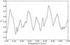 |
Fig. 5 Kuiper-test periodogram for the ff- and gr-event epochs in Table 3. |
| In the text | |
|
Fig. 6 CPS-analysis of segment SEG3. The contents of the panels are explained at the end of Sect. 3. |
| In the text | |
Current usage metrics show cumulative count of Article Views (full-text article views including HTML views, PDF and ePub downloads, according to the available data) and Abstracts Views on Vision4Press platform.
Data correspond to usage on the plateform after 2015. The current usage metrics is available 48-96 hours after online publication and is updated daily on week days.
Initial download of the metrics may take a while.