| Issue |
A&A
Volume 561, January 2014
|
|
|---|---|---|
| Article Number | A110 | |
| Number of page(s) | 13 | |
| Section | Galactic structure, stellar clusters and populations | |
| DOI | https://doi.org/10.1051/0004-6361/201322802 | |
| Published online | 16 January 2014 | |
Multipopulation aftereffects on the color–magnitude diagram and Cepheid variables of young stellar systems
1
INAF – Osservatorio Astronomico di Roma, via Frascati 33,
00040
Monte Porzio Catone,
Italy
e-mail: This email address is being protected from spambots. You need JavaScript enabled to view it.
; This email address is being protected from spambots. You need JavaScript enabled to view it.
2
INAF – Osservatorio Astronomico di Capodimonte, Salita Moiariello
16, 80131
Napoli,
Italy
e-mail:
This email address is being protected from spambots. You need JavaScript enabled to view it.
3
INAF – Osservatorio Astronomico di Teramo, Mentore Maggini s.n.c.,
64100
Teramo,
Italy
e-mail:
This email address is being protected from spambots. You need JavaScript enabled to view it.
Received:
4
October
2013
Accepted:
15
November
2013
Abstract
Context. The evidence of a multipopulation scenario in Galactic globular clusters raises several questions about the formation and evolution of the two (or more) generations of stars. These populations show differences in their age and chemical composition. These differences are found in old- and intermediate-age stellar clusters in the Local Group. The observations of young stellar systems are expected to present footprints of multiple stellar populations.
Aims. This theoretical work intends to be a specific step in exploring the space of the observational indicators of multipopulations, without covering all the combinations of parameters that may contribute to the formation of multiple generations of stars in a cluster or a galaxy. The goal is to shed light on the possible observational features expected by core He-burning stars that belong to two stellar populations with different original He content and ages.
Methods. The tool adopted was the stellar population synthesis. We used new stellar and pulsation models to construct a homogeneous and consistent framework. Synthetic color–magnitude diagrams (CMDs) of young- and intermediate-age stellar systems (from 20 Myr up to 1 Gyr) were computed in several photometric bands to derive possible indicators of double populations both in the observed CMDs and in the pulsation properties of the Cepheids.
Results. We predict that the morphology of the red/blue clump in VIK bands can be used to photometrically indicate the two stellar populations in a rich assembly of stars if there is a significant difference in their original He content. Moreover, the period distribution of the Cepheids appears to be widely affected by the coeval multiple generations of stars within stellar systems. We show that the Wesenheit relations may be affected by the helium content of the Cepheids.
Key words: galaxies: star clusters: general / stars: evolution / stars: abundances / stars: distances / stars: variables: Cepheids
© ESO, 2014
1. Introduction
A large number of young- and intermediate-age massive clusters (YIMCs) are known in the local Universe as far away as among nearby star-burst galaxies. These systems are one of the preferred environments for star formation to take place (Lada & Lada 2003). For this reason, they may be responsible for a significant fraction of the current star formation in the local Universe and be the intriguing progenitors of the present-day population of old globular clusters (GCs). Therefore, to study YIMCs in terms of their stellar content is crucial for understanding both current and primordial star formation processes in galaxies.
In the past decade, our knowledge on star formation in GCs has been revolutionized. High-resolution spectroscopy and precise photometry of individual stars in GGCs provided the evidence that multiple stellar generations are present in these stellar systems (e.g. Gratton et al. 2012; Piotto 2010). In the Magellanic Clouds (MCs), stellar clusters show a wide spread in age (e.g. Brocato et al. 2001 and reference therein), and signs of two or more stellar populations have been found in young- and intermediate-age objects (Mackey & Broby Nielsen 2007; Glatt et al. 2008; Milone et al. 2009; Goudfrooij et al. 2011; Keller et al. 2011), suggesting that a star cluster can host (at least) two stellar populations with different ages (Δt < 1 Gyr) and chemical compositions.
The current view on the matter suggests that, generally, the second generation (SG) of stars differs from the first generation (FG) mainly in the He abundance, and this difference can be as high as ΔY ≃ 0.1 (e.g. D’Antona & Caloi 2004; Piotto 2008). Two main models have been proposed to explain the presence of multiple stellar generations in star clusters and their chemical abundances: the so-called super-asymptotic giant branch (S-AGB) and AGB stars scenario (Ventura et al. 2001), and the fast-rotating massive stars scenario (FRMS, Decressin et al. 2007).
According to the first scenario, during the AGB evolution stars with mass M ≳ 4 M⊙ experience the so-called hot bottom burning (HBB) at the bottom of their convective envelope (Blöcker 1991). The H-rich matter is processed through the hot CNO cycle, where the Ne-Na and Mg-Al chains are active. The processed material is ejected into the intracluster medium and retained in the potential well of the cluster, due to the small velocities of the AGB stellar winds. The enriched matter mixes with the pristine gas and forms the second-generation stars (D’Ercole et al. 2008). The evolutionary timescales of this model range from δt ≈ 40 Myr to δt ≈ 100 Myr. The former timescale is driven by the evolution time of the most massive S-AGB stars (M ~ 8 M⊙1), while the latter is related to the lifetime of stars with M ~ 4 M⊙, which also corresponds to the minimum time needed for Type Ia supernovae (SNe) to occur. These events add positive energy to the system, stopping the star formation process.
The FRMS scenario suggests that during the main sequence (MS), massive stars (M = 20−60 M⊙) can eject CNO-processed material at low velocity, transported from the inner regions to the surface by rotationally induced mixing: the required rotation rates are close to the break-up velocity. If an accretion disk is formed, the gas ejection velocity is extremely low, thus the processed material can be retained in the potential well of the cluster and can be mixed with the pristine gas, forming the second-generation stars. In this case, the evolution time ranges from 5 Myr to ~20 Myr and ends before Type II SNe explosions occur.
These two models are not yet fully accepted, since they lack a self-consistent explanation of the picture, and weaknesses are still affecting the two proposed scenarios. For example, uncertainties affect the number ratio between the first- and second-generation stars. Recently, Bastian et al. (2013b) proposed a new picture where low-mass pre-main sequence stars accrete enriched material released from interacting massive binary and rapidly rotating stars onto their circumstellar disks, and ultimately onto the young stars.
In this context, a relevant contribution comes from the analysis of young stellar systems (e.g. t < 1 Gyr) where possible second-generation stars are newly formed. Searches of multiple stellar populations have been mainly conducted in old GCs of the Galaxy. In old systems, multiple populations are typically identified from the photometry of main sequence, red giant branch (RGB) and horizontal branch (HB) stars (e.g. D’Antona & Caloi 2004; Bedin et al. 2004). However, high-resolution photometric data are required to distinguish multiple turn-off (TO) and to evaluate the age difference between the first- and second-generation stars if younger than about 1 Gyr. In contrast, in young- and intermediate-age GCs even a small age difference can produce multiple TO or other easily detected photometric signatures. Multipopulations have been discovered by fitting the location of the MS in the observed CMD (Milone et al. 2008). Moreover, since the clump of He-burning stars is more luminous than the MSTO, it potentially represents a more effective way to recognize the presence of multipopulations in young massive clusters. For these reasons, YIMCs are systems that can be very powerful to help in understanding the formation processes of the second-generation stars and, more importantly, they provide a key opportunity to distinguish between the nature of the polluters responsible for the new chemical abundances of second-generation stars, thus giving solid constraints in favor or against the proposed scenarios. On the base of visual inspection of spectra and CMDs of 130 YIMCs, Bastian et al. (2013a) suggested that models with continuous star formation are ruled out, while models requiring the nearly instantaneous formation of a secondary population are not formally discounted. In their analysis the disk accretion model (Bastian et al. 2013b) seems to be preferred.
In this paper, we tackle this open question by studying the expected photometric properties of resolved stars in young- and intermediate-age stellar clusters under the hypothesis of single-burst and multipopulation scenarios. Our goal is to investigate the features of core He-burning stars in the CMD and the observational properties of the Cepheids expected in two simple cases: i) single-burst stellar populations where all stars have the same age and a chemical composition typical of the Large Magellanic Cloud (LMC), i.e. Y = 0.25 and Z = 0.008; ii) stellar systems where first-generation stars (Y = 0.25, Z = 0.008 and age t = tFG) are mixed with a second generation of stars born after a time δt = tFG − tSG (ranging from 20 Myr up to 100 Myr) that have a different He abundance (Y = 0.35). The age of first-generation stars ranges from a few Myr up to ~1 Gyr. The idea is to explore and point out differences in the photometric properties of stars expected in the two cases, by taking advantage of stellar population synthesis methods. For this purpose, we derived synthetic CMDs in the classical Johnson-Cousins photometric bands (UBVRIJHK).
Since the Cepheid variables are an important stellar component of young clusters, we predict their properties using population synthesis models coupled with high precision pulsation models. We evaluate the impact of multipopulations on the pulsation properties such as the period distribution and the Wesenheit index. We aim to point out possible bias in the estimate of astronomical distances based on Cepheid relationships.
The paper is arranged as follow: Sect. 2 describes the new stellar evolution models, the new stellar pulsation models and briefly introduces of the adopted stellar population synthesis code. The results of the synthetic CMDs are discussed in Sect. 3, while the prediction on the properties for the Cepheids and the impact on the Wesenheit relations are shown in Sect. 4. A brief discussion closes the paper.
2. Physical and numerical inputs
2.1. Evolution code
The stellar evolution code used here is ATON. This can follow all the evolutionary phases from the pre-MS to D-ignition at the beginning of the MS, up to carbon ignition (Ventura et al. 2008). The ignition of the reaction 16O + 16O and the following pre-supernova phases are not accounted for. In the following we briefly recall the main features of the code.
ATON describes spherically symmetric structures in hydrostatic equilibrium. The internal structure is integrated via the Newton-Raphson relaxation method from the center to the base of the optical atmosphere (τ = 2/3). The independent variable is the mass, while the dependent ones are temperature, pressure, radius, and luminosity. The zoning is reassessed after each physical time step, with particular care to the central and surface regions in the vicinities of convective boundaries and H or He-burning shells and close to the superadiabacity zones.
Once the physical structure of the model is determined via the relaxation method, a time
step is applied to achieve the chemical evolution. To this end, each physical time step is
divided in to ten chemical time steps. Mechanisms leading to a variation of the chemical
composition, such as nuclear burning, gravitational settling, and convective mixing, are
properly taken into account. All the evolution models presented here were calculated by
adopting the full spectrum of turbulence (FST) treatment with the appropriate convective
flux distribution (Canuto &Mazzitelli
1991). Mixing of the chemicals within convective zones is treated as a diffusive
process: for an individual element Xi the
code solves the equation by Cloutman & Eoll
(1976): ![Mathematical equation: \begin{equation} \frac{{\rm d}X_i}{{\rm d}t}= \frac{\partial X_i}{\partial t} + \frac{\partial}{\partial m_r}\left[(4\pi r^2\rho^2)^2 D\frac{\partial X_i}{\partial m_r}\right], \end{equation}](/articles/aa/full_html/2014/01/aa22802-13/aa22802-13-eq19.png) (1)where D
is the diffusion coefficient
(D = 16πr4ρ2τ-1),
ρ is the density, and τ is the turbulent diffusion
timescale. The mass fraction of the element is defined as
Xi = Xi/ρNA,
where NA is the Avogadro’s number. A network of 64 reactions
is adopted. The cross sections are taken from the NACRE compilation (Angulo et al. 1999), with the following exceptions:
(1)where D
is the diffusion coefficient
(D = 16πr4ρ2τ-1),
ρ is the density, and τ is the turbulent diffusion
timescale. The mass fraction of the element is defined as
Xi = Xi/ρNA,
where NA is the Avogadro’s number. A network of 64 reactions
is adopted. The cross sections are taken from the NACRE compilation (Angulo et al. 1999), with the following exceptions:
-
14N(p,γ)15O (Formicola et al. 2004)
-
22Ne(p,γ)23Na (Hale et al. 2002) (upper limit)
-
23Na(p,γ)24Mg (Hale et al. 2002)
-
23Na(p,α)22Ne (Hale et al. 2002) (lower limit)
-
4He(2α,γ)12C (Fynbo et al. 2005)
-
12C(α,γ)16O (Kunz et al. 2002).
Regions unstable to convection are identified via the Schwartzschild criterion. We took into account convective overshooting for the core convective regions and for the surrounding convective shell, assuming that the turbulent velocity exponentially vanishes outside the formally convective regions. This is simulated by introducing the parameter ξ, which defines the scale length over which the velocity decays into the region that is radiatively stable. In this study we set ξ = 0.02, in agreement with the calibration given in Ventura et al. (1998). No overshooting was used for the evolutionary phases following the core He-burning phase. We note that reasonable modifications in the overshooting parameter possibly affect the calibration of the absolute ages of star clusters without a major impact on the following investigation.
Mass loss [M⊙/yr] is modeled according to Blöcker (1995):
 (2)where
M,L, and R are denoted in solar units,
ηR is a free parameter. We used
ηR = 0.02. This value was calibrated
specifically for the range of masses and for the metallicity used here via a comparison
between the observed and the predicted luminosity function of lithium-rich sources and of
carbon stars in the LMC (Ventura et al. 1999, 2000). However, variations in this mass-loss rate
within the commonly accepted values are not expected to modify our main results.
(2)where
M,L, and R are denoted in solar units,
ηR is a free parameter. We used
ηR = 0.02. This value was calibrated
specifically for the range of masses and for the metallicity used here via a comparison
between the observed and the predicted luminosity function of lithium-rich sources and of
carbon stars in the LMC (Ventura et al. 1999, 2000). However, variations in this mass-loss rate
within the commonly accepted values are not expected to modify our main results.
We computed evolutionary tracks for stars with mass from M = 0.4 M⊙ to 12 M⊙, with an initial chemistry typical of the LMC (Z = 0.008) and α-enhanced [α/Fe] = 0.2, with the reference solar mixture taken from Grevesse & Sauval (1998). The evolution of stars with both Y = 0.25 and Y = 0.35 from the pre-MS to the beginning of the thermal pulses was calculated (see Fig. 1).
 |
Fig. 1 Selected sample of evolutionary tracks calculated with the ATON code. The initial chemistry is: Z = 0.008, α-enhancement [α/Fe] = 0.2, Y = 0.25 (bottom panel) and Y = 0.35 (top panel). |
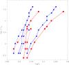 |
Fig. 2 Comparison between the predicted instability-strip boundaries for the two assumed helium contents, namely Y = 0.25 (red circles) and 0.35 (blue squares). The solid lines are the fundamental edges, the dashed lines are the first-overtone edges. |
2.2. Stellar pulsation models
For the same chemical compositions as were adopted in the evolutionary models, we computed a set of nonlinear convective pulsation models, using the physical and numerical assumptions discussed in Bono et al. (1999b), Valle et al. (2009) and Marconi et al. (2010) for stellar masses ranging from 3 to 12 M⊙. For each stellar mass a mass-luminosity relation (Bono et al. 2000a) was adopted2, an extensive range in effective temperature was explored and the modal stability was investigated both for the fundamental (FU) and the first-overtone (FO) instability-strip. As a result, for each selected chemical composition, we determined the instability-strip boundaries for both pulsation modes, as summarized in Table 1. The first four columns of the table report the adopted chemical composition, mass, and luminosity. In the subsequent columns the effective temperature of the predicted first-overtone blue edge (FOBE), fundamental blue edge (FBE), first-overtone red edge (FORE), and fundamental red edge (FRE) can be found.
Physical parameters and location of the fundamental and first-overtone instability-strip boundaries for the adopted pulsation model sets.
Coefficients of the adopted pulsation relations: log P = a + blog Te + clog L/L⊙ + dlog M/M⊙.
A comparison between the theoretical instability-strip for Y = 0.25 and Y = 0.35 is shown in Fig. 2. As expected on the basis of previous results (Fiorentino et al. 2002; Marconi et al. 2005), the instability-strip of fundamental pulsators becomes hotter as the helium abundance increases. Here, we also find that the effect is even more evident for first-overtone pulsators.
To provide a link between the pulsation period and the intrinsic evolutionary model properties, namely the mass, luminosity, and effective temperature, the pulsation relations were derived from regression through all the pulsating nonlinear models for each chemical composition and for both pulsation modes. The coefficients of these relations are reported in Table 2.
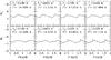 |
Fig. 3 Light curves in the absolute V magnitude for models with M = 7 M⊙ and Y = 0.35. |
The adopted nonlinear pulsation models also allow us to predict the variations of all the relevant quantities along a pulsation cycle. A subset of the obtained light curves in the absolute V magnitude is shown in Fig. 3 for models with M = 7 M⊙, Z = 0.008, and Y = 0.35.
The selected stellar mass corresponds to a period range (6 days <P < 16 days) where a secondary maximum (bump) appears both in the light curve and in the radial velocity curve. The relationship between the phase of this bump and the pulsation period is known as the Hertzsprung progression (HP; Hertzsprung 1926), and this group of variables has been named bump Cepheids. In previous papers based on the same type of pulsation models, it has been shown that an increase in the metal content causes a shift of the HP center toward shorter periods. The behavior shown in Fig. 3 indicates that the helium abundance has an opposite effect: the HP center moves to longer periods because the helium content increases at fixed metallicity. Indeed, at fixed stellar mass (7 M⊙) the center of the HP occurs at a period of about 13.5 days, significantly longer than the value obtained at Y = 0.25, namely 11.2 d (see Bono et al. 2000b). Empirical data for the LMC suggest that the HP center corresponds to a period of about 11 days (see e.g. Welch et al. 1997; Beaulieu 1998), which agrees better with the theoretical value for Y = 0.25. However, observations of the Hertzsprung progression in extragalactic Cepheid samples at the same metallicity (Z ≃ 0.008) and a similar period range could, in principle, allow us to distinguish the helium content on the basis of the above considerations. This is particularly true in the NIR bands, since Storm et al. (2011) found a weak dependence on the metallicity in the optical bands.
2.3. Stellar population synthesis
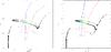 |
Fig. 4 Synthetic CMD in the absolute V band for a population of 100 Myr with Y = 0.25 (left panel) and Y = 0.35 (right panel). The green triangles represent the Cepheids. The FRE (red line), FORE (dashed red line), FBE (blue line) and the FOBE (dashed blue line) are also shown. In these plots the photometric uncertainties are neglected. |
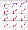 |
Fig. 5 Synthetic CMDs in the V, I, and K bands. We hypothesize that the GC is composed of two families of stars with Y = 0.25 (red circles) and Y = 0.35 (blue squares), with an age difference of 20 Myr: the age of the first- and second-generation stars are labeled. Cepheids are marked as green triangles. |
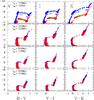 |
Fig. 6 As in Fig. 5, but for an age difference of 100 Myr between the first- and second-generation stars. |
Synthetic CMDs and observational properties of the Cepheids were derived using the most recent version of the stellar population synthesis code SPoT3 (Raimondo et al. 2005; Raimondo 2009). The code was used to fit in detail the observed CMDs of GGCs and MC clusters for a wide range of ages and metallicities (Brocato et al. 2000; Raimondo et al. 2002; Raimondo 2009; Bellini et al. 2010). It was used to reproduce the fast and luminous evolutionary phases and, in particular, the red clump of LMC star clusters with a high level of accuracy (e.g. Brocato et al. 2003). For the specific purpose of this study, we computed synthetic magnitudes and colors (in the UBVRIJHK bandpasses) by adopting the BaSeL 3.1 (Westera et al. 2002; Patricelli 2006) stellar atmospheres library. To this aim, the code was implemented to include the evolutionary tracks calculated with the ATON code (Sect. 2.1) and a specific routine was added to the SPoT code with the aim of computing the number of predicted Cepheids and, for each variable, the pulsation mode and the period on the basis of the pulsation models described in Sect. 2.2.
Spread of the (red and blue) clumps in the V, I and K bands for populations with Y = 0.25 (FG), Y = 0.35 (SG), and the mixed population (multiple).
Spread of the (red and blue) clumps in the V, I and K bands for populations with Y = 0.25 (FG), Y = 0.35 (SG), and the mixed population (multiple).
We adopted a Salpeter initial-mass function (IMF, α = 2.35) ranging from 0.4 M⊙ up to 100 M⊙. The total number of stars in each CMD was chosen to properly populate the red clump of core He-burning stars. A Monte Carlo method – weighted according to evolutionary timescale and IMF – was used to reproduce the stochastic behavior expected in observed CMDs. Photometric uncertainties were simulated by a specific algorithm that takes into account the typical increasing spread expected for photometric CCD measurements of faint stars. We computed synthetic CMDs and Cepheid properties for two chemical compositions (Z = 0.008, Y = 0.25) and (Z = 0.008, Y = 0.35) in the age range from 20 Myr up to 1 Gyr. We decided to fix the number of He-burning stars to be on the order of ~100 in each model (if not explicitly stated otherwise), so that a well populated core He-burning phase (i.e. the red/blue clump) was derived.
In Fig. 4 we show the synthetic [V, B − V] CMD from the MS to the end of the core He-burning for a population of 100 Myr, with Y = 0.25 (left panel) and Y = 0.35 (right panel). During the blue loop, the stars cross the instability-strip, becoming Cepheid variables (green triangles). At fixed age, the TO point of the He-enriched population is fainter than the first-generation stars TO point, since stars with a higher He abundance evolve more rapidly, while the blue loop is less extended in color (0.67 vs. 0.8 mag) and spread more in the absolute V magnitude.
3. Color–magnitude diagram
In this section, we focus on pinpointing some indicators for multipopulations in young- and intermediate-age stellar systems by using the properties of He-burning stars. It is worth mentioning that these stars are very luminous objects, hence they could represent a powerful way to recognize multigenerations of stars in young clusters provided that they are massive enough to possess a significant number of core He-burning stars. It is well known that the chemical composition of a star plays a fundamental role in its evolution. It sets the rate of energy generation and determines the wavelength distribution of the emerging flux. Stars with a high helium abundance (e.g. Y = 0.35), due to the high molecular weight, evolve in a shorter time and are more luminous and hotter than stellar models with a lower helium abundance (e.g. Y = 0.25) at fixed mass. For this reason the MS position and the core He-burning loop of He-rich stellar models are respectively bluer and brighter than those of classic (i.e. standard He) models with the same mass (see Fig. 1). In the following we concentrate on the expected properties of stars experiencing the core He-burning phase, since the evolutionary times are long enough to generate a relatively well populated “observational” feature in young- and intermediate-age massive stellar systems.
Figures 5 and 6 show a sample of synthetic CMDs (in the V, I, and K bands) for different assumptions on the age of the first- and second-generation stars after fixing their age difference: δt = tFG − tSG = 20 Myr and 100 Myr, respectively. The ages increase from the top to the bottom of each figure. The helium content is Y = 0.25 for the first-generation stars (red circles), while Y = 0.35 (blue squares) is assumed for the second-generation stars. The green triangles indicate the Cepheid variables, which we analyze in the next section.
We recall that He-burning stars with mass ranging from ≃5 M⊙ up to ≃10 M⊙ experience an extended loop in effective temperature, but they spend a large part of the time needed to exhaust the helium in their convective core at the extreme (cool and hot) edges of the loop. Consequently, we expect to find two clumps at red and blue colors. For the sake of clarify, we define as red a clump located at (B − V) ≥ 0.4 mag and blue a clump at (B − V) < 0.4 mag.
We decided to search for photometric indicators for multiple populations using the red and blue clump properties. To this end, we defined the mean magnitude ⟨ XHe−b ⟩, its dispersion σXHe−b, and the magnitude spread ΔXHe−b of the red/blue clump as follows:
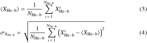
 (5)where
 is the
magnitude of the ith core He-burning star, measured in the given
X-band. The sum is extended to all the core He-burning stars
(NHe−b). When the blue and red clumps are present in the
CMD, the sum was computed separately for the stars of each subset.
is the
magnitude of the ith core He-burning star, measured in the given
X-band. The sum is extended to all the core He-burning stars
(NHe−b). When the blue and red clumps are present in the
CMD, the sum was computed separately for the stars of each subset.
 and
and
 are,
respectively, the X-band magnitude of the brightest and the faintest edge
of the He-burning star clump. In Tables 3 and 4 we report these quantities for the computed stellar
populations.
are,
respectively, the X-band magnitude of the brightest and the faintest edge
of the He-burning star clump. In Tables 3 and 4 we report these quantities for the computed stellar
populations.
In young systems (tFG ≲150 Myr) we can distinguish the two populations both at the MS and at the location of stars burning helium in the core. For δt = 20 Myr (Fig. 5), the loops produced by the first- (red circles) and the second-generation (blue squares) stars are clearly separated (in magnitude). Therefore, a double stellar population would be easily discovered from the morphology of the red/blue clump. The magnitude spread (ΔXHe−b) ranges from 0.6 to 1.8 in the V band, and from 0.5 to 2.6 in the K band (Table 3). The color extension of the core He-burning loops does not show sizable differences between the single and double populations because the masses experiencing this evolutionary phase are similar. When we stretch δt to 100 Myr (Fig. 6), the magnitude spread increases to a value higher than 2 mag (Table 4). Furthermore, the differences in the morphology of the red/blue loop become even wider than for δt = 20 Myr.
When tFG is ≳300 Myr, we are unable to distinguish the two subpopulations by simply observing the morphology of the red/blue loop in both cases (δt = 20 Myr and δt = 100 Myr). At these ages and for the chemical composition assumed, the blue clump disappears, since the evolution models predict a loop less extended in effective temperature for the typical mass experiencing the core He-burning phase (M ≲ 4 M⊙, see Fig. 1). However, when the two populations are mixed the magnitude distribution of stars in the red clump is larger than that produced when the two populations are considered separately. In fact, even if the core He-burning stars of the two subpopulations appear quite superimposed in the CMD, a close look shows that the magnitude spread of the clump increases a few tenths of magnitude when populations are mixed, as tabulated in Tables 3 and 4. As a general result, we therefore find that the quantity ΔXHe−b is an alternative tool to identify multiple stellar populations in YIMCs. This effect is stronger in the K band than in the bluer bands. Accurate photometric observations of populous stellar systems are needed to enable one to measure the magnitude spread with adequate precision (e.g. ≲0.05 mag) in the V band.
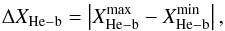
To illustrate this result, in Fig. 7 we plot the time evolution of the clump magnitude spread in the V and K bands. In the figure we omit the I band because its trend is similar to that in the V band. Left panels of the figure refer to δt = 20 Myr, while right panels show δt = 100 Myr. The red filled circles and the blue squares describe the magnitude spread of the core He-burning stars (red clump) for a single population with Y = 0.25 and Y = 0.35, respectively. The green triangles represent the amplitude of the quoted spread when the two populations coexist.
 |
Fig. 7 Time evolution of the ΔVHe−b (top panels) and ΔKHe−b (bottom panels) bands for a population with Y = 0.25 (red full circles), Y = 0.35 (blue full squares), and a mixed population (green full triangles). The age spread is 20 Myr (left panel) and 100 Myr (right panel), respectively. |
From the figure, it is clear that the quantity ΔXHe−b is an alternative tool to single out multiple stellar populations in YIMCs. The magnitude spread changes sizably from single-age to multiple-age (double) populations in the whole range of ages considered here. In particular, when δt = 100 Myr (right panels of Fig. 7), ΔXHe−b clearly is a reliable indicator of the possible presence of mixed populations, at least under the hypotheses explored in the present work. For young clusters, for example, for tFG = 130 Myr, ΔXHe−b of the multiple population is expected to be about four times higher than the value for the single-age population in the V and K bands. Increasing the age, this difference decreases, because the mass of stars evolving in the core He-burning phase becomes similar in the two subpopulations. It is interesting to note that this feature is effective in distinguishing multipopulations in different photometric bands.
This quantity is less effective when the age difference shrinks to δt = 20 Myr. The synthetic CMDs show that the clump of He-burning stars in young clusters (t ≲ 150 Myr) is still a powerful way to evaluate whether there are multiple stellar populations. For older ages, the effectiveness of the V band decreases while the K band remains nearly as effective also at ages older than 300 Myr.
On these bases, we suggest that the magnitude spread ΔXHe−b is a useful quantity to identify whether there are mixed populations in relatively young- and intermediate-age massive stellar systems. We recall we assumed age differences between the first- and the second-generation stars according to the current scenarios proposed to explain multipopulations in star clusters.
We note that before one can compare this magnitude spread with observations, some
refinements are needed. We suggest that  and
should be
obtained from the accurate luminosity function of the red/blue clump stars. The faint edge
of the red clump can be identified as a sudden rise in stellar counts due to the very few
stars expected at lower luminosities. On the other hand, RGB and AGB stars could in
principle hamper the definition of the bright edge. Nevertheless, the evolutionary time
differences between the RGB/AGB and the He-burning phases enable one to predict a sizeable
drop () in the
luminosity function. For instance, for a 5 M⊙ star the time
ratios are
τHe−b/τRGB ~
15 and τHe−b/τAGB ~ 100. This
allows one to separate the red clump stars from the RGB/AGB stars. The blue clump spread can
also be easily distinguished in the luminosity distributions. If we analyze the luminosity
distribution of the stars with
B − V < 0.4 mag, we can see in
the histogram a primary and a secondary maximum. The former represents MS stars, the latter,
at higher luminosities, corresponds to the blue loop stars. This secondary feature allows us
to obtain the limits of the magnitude spread.
and
should be
obtained from the accurate luminosity function of the red/blue clump stars. The faint edge
of the red clump can be identified as a sudden rise in stellar counts due to the very few
stars expected at lower luminosities. On the other hand, RGB and AGB stars could in
principle hamper the definition of the bright edge. Nevertheless, the evolutionary time
differences between the RGB/AGB and the He-burning phases enable one to predict a sizeable
drop () in the
luminosity function. For instance, for a 5 M⊙ star the time
ratios are
τHe−b/τRGB ~
15 and τHe−b/τAGB ~ 100. This
allows one to separate the red clump stars from the RGB/AGB stars. The blue clump spread can
also be easily distinguished in the luminosity distributions. If we analyze the luminosity
distribution of the stars with
B − V < 0.4 mag, we can see in
the histogram a primary and a secondary maximum. The former represents MS stars, the latter,
at higher luminosities, corresponds to the blue loop stars. This secondary feature allows us
to obtain the limits of the magnitude spread.
We briefly discuss the possibility that a large part of the FG stars are lost in the very early stage of the cluster life. This clearly affects our statement of having ~100 He-burning stars in both the populations. In this case, the magnitude spread remains a good indicator of multiple populations if the number of the FG He-burning stars is on the order of a few tens at least. In fact, just a handful of these stars is needed to define the lower edge of ΔXHe−b. Furthermore, this faint side has the advantage of not being affected by the uncertainties due to the presence of RGB and AGB stars.
Before concluding our analysis, we note that binary systems are not expected to affect our main conclusions. Although observations indicate that the majority of stars are found in binary systems (Rastegaev 2010), close encounters involving binary systems may disrupt soft (i.e. generally wide) binaries in dense clusters (Heggie 1975). Thus, the actual binary fraction in YIMCs is uncertain (Portegies Zwart et al. 2010; Vanbeveren et al. 2012). Binary stars could, in principle, resemble an increase of the clump magnitude spread. However, their contribution to ΔXHe−b would be at most as large as ~0.75 mag, but only if the mass difference between the two components is smaller than ~0.2 M⊙. If so, they can experience the core He-burning phase simultaneously. If the mass difference is larger than this value, the binary system is most likely composed of a MS star plus a red-clump star. This type of binaries does not change ΔXHe−b. Thus, the effect of binaries on the amplitude of the red clump will be confined to a handful of stars located at bright magnitudes (e.g. δV ≤ 0.75 mag).
 |
Fig. 8 Period distribution of Cepheids for a stellar population containing stars with two different helium abundances (Y(FG) = 0.25 and Y(SG) = 0.35), and an age difference of 20 Myr. The age of the first-generation stars is tFG = 40 Myr (left panel) and tFG = 120 Myr (right panel). The green line represents the period distribution expected by the double population and defines the adopted bin size (left panel: 0.025; right panel: 0.05). For clarify, the bins of the red and blue columns are drawn smaller than the adopted ones. |
 |
Fig. 9 As in Fig. 8, but the age difference between the two subpopulations is 100 Myr. The age of the first-generation stars is tFG = 120 Myr (left panel, adopted bin: 0.1) and tFG = 200 Myr (right panel, adopted bin: 0.05). |
4. Stellar pulsation
Using the pulsation period relations as a function of the intrinsic stellar parameters given in Table 1, we computed the period corresponding to each “star” of the synthetic CMDs falling within the predicted Cepheid instability strip for the two assumed chemical compositions. Synthetic stars falling between the first-overtone blue edge and the fundamental blue edge were assumed to pulsate in the first-overtone mode, and the relative pulsation relation was adopted. When a synthetic star is within the “OR region”4, we assumed that the pulsation mode is fundamental if the star, in its evolutionary path, crosses the CMD from the red to the blue side. In contrast, the first-overtone pulsation was assigned to synthetic stars evolving from the blue side. Finally, the fundamental-mode is assumed for synthetic stars located between the first-overtone red edge and the fundamental red edge.
When a mixed population -with the first generation of Y = 0.25 and t = 40 Myr and the second one of Y = 0.35 and t = 20 Myr- is considered, the resulting period distribution (left panel of Fig. 8) shows that the maximum number of pulsators have a period of about 30 days and the majority of Cepheids belongs to the second generation and have a period in the range ~30 ÷ ~45 days. On the other hand, if we consider the same age gap, but with the first generation at 120 Myr and the second one at 100 Myr, a mixed Cepheid population is expected (see the right panel of the same figure) for periods shorter than about 5 days, whereas a predominance of the second generation is found between 5 and 10 days.
If the second generation is young, as in Fig. 8, but the first one is older by 100 Myr, we expect the behavior shown in Fig. 9. We note that by increasing the age gap, the covered period range becomes wider. In particular, if the Y = 0.25 population has an age of 120 Myr and the Y = 0.35 population has 20 Myr, we expect two distinct period distributions peaked at ~5 and ~30 days (left panel of Fig. 9), respectively, with no pulsator in the period range 8 ÷ 20 days. If the Y = 0.25 population has an age of 200 Myr and the Y = 0.35 population has 100 Myr, we predict a more continuous distribution with an excess of first-generation Cepheids at the shortest periods and a predominance of second-generation pulsators for periods longer than 3 days.
The present exploratory work suggests that an another tool for distinguishing multipopulations (with wide differences in their original helium content) in young massive stellar systems is embedded in the period distribution of their Cepheids. In fact, our simulations show that the observed period distributions of Cepheids that belong to two different populations (with age and helium abundances assumed in this paper) tend to considerably increase the range of the measured periods.
Thus, a careful analysis of the period distribution of Cepheids in massive stellar systems may give an indication whether there are multiple populations present. In this way, the detection of Cepheids with a period longer than expected is another tool for distinguishing multipopulations.
4.1. Application to the distance scale: the synthetic Wesenheit relations
It is well known that the period-luminosity (PL) relation of classical Cepheids in the optical bands is affected by systematic uncertainties related to the intrinsic dispersion because of the finite width of the instability-strip, nonlinearity at the longest periods, reddening, and chemical composition (Bono et al. 1999a; Caputo et al. 2000b). To remove the reddening effect and reduce both the influence of the instability-strip topology and the metallicity contribution, the Wesenheit relations (Madore 1982) are often adopted in the literature. Indeed, when two bands are available, for example, B and V, one can define WBV = V − RV(B − V), where RV is the visual extinction-to-reddening ratio AV/E(B − V). The resulting period-Wesenheit (PW) relation is independent of reddening. Similar PW relations can be defined by using an extinction law, for instance the one by Cardelli et al. (1989). As the effect of the extinction is similar to that produced by the finite width of the instability-strip, the scatter around the PW relations is smaller than in any observed PL relation (Caputo et al. 2000a; Marconi et al. 2005; Bono et al. 2010, see e.g.). In particular, the PW relation defined using the V and I bands is also almost independent of metallicity, and hence represents an ideal tool for estimating the distance of extragalactic Cepheids (Bono et al. 2010). In this context, we recall that Storm et al. (2011) found a metallicity effect on the coefficients of the PW relations in the optical bands.
Coefficients of the adopted PW relations for fundamental-mode pulsators: Wbands = βlog P + α.
We can evaluate the synthetic PW relations by simulating stellar populations with different original helium content. For these computations we assumed for each given age a total cluster mass of about 5 × 10⁵ M⊙. The ages were chosen to populate the Cepheid period range (0.4 ≲ LogP ≲ 2) typically adopted in the empirical evaluation of the Wesenheit relation (Udalski et al. 1999; Bono et al. 2010). The coefficients of the resulting relations for fundamental-mode pulsators are reported in Table 5 for each adopted chemical composition. First of all, we note that our WVI relation for the case with Y = 0.25 agrees very well with the one obtained from observations of LMC Cepheids (Udalski et al. 1999). Moreover, our coefficients of the WJK, WVK, and WVJ relations reproduce the recent results of Inno et al. (2013) very well, although we note some discrepancy with their WVI relation. When the helium content increases from Y = 0.25 to Y = 0.35 the Wesenheit relations become steeper.
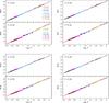 |
Fig. 10 PW relations in different filter combinations [V,(B − V)] (upper left panel), [I,(V − I)] (upper right panel), [K,(V − K)] (lower left panel) and [K,(J − K)] (lower right panel) for the two single-He abundance populations, as labeled. Colors refer to populations with different ages as reported in the upper left panel. In each upper (lower) panel, the solid blue (red) line is the PW relation derived for Cepheids with Y = 0.25 (Y = 0.35), while the dashed black line indicates the PW relation derived by combining the stellar populations with different helium abundances. |
Figure 10 shows the synthetic fundamental-mode Wesenheit relations for the various filter combinations, namely [V, (B − V)], [V, (V − I)], [V, (V − K)], and [K,(J − K)], for the two assumptions on the helium content. In each panel the dashed line depicts the relation assuming a combined stellar population with two adopted helium abundances (last four lines of Table 5). We note that the combined relations are closer to those for Y = 0.35 than to those at Y = 0.25. This occurrence is due to the different period distributions of Cepheids at different helium content, with the pulsators at Y = 0.35 dominating the short-period range. We note that depending on the period range, the effect can be as large as 0.2–0.3 mag. This implies that adopting the LMC-calibrated Wesenheit relation to derive the distances of Cepheid samples belonging to populations affected by He enrichment mechanisms may be inadequate.
5. Conclusions
We explored the possibility of detecting multiple populations in star clusters by observing bright, intermediate-age massive stars that experience the core He-burning phase. These stars typically gather together, forming a red/blue clump in the CMD of very populous stellar systems with ages from few Myr up to ~1 Gyr. Our work was motivated by the simple consideration that because GGCs show multiple populations, signs of multiple generations of stars can probably also be found in young stellar systems, under the assumption that the formation process of star clusters is universal. This view seems supported by recent observations, because in a few MC clusters some broadening of the main sequence has been detected (e.g. Milone et al. 2008, 2013).
As a starting step, we focused on stellar populations with different original helium content, as suggested in recent works on GGCs (e.g. D’Antona & Caloi 2004; Piotto 2008; Monelli et al. 2013) and by theoretical scenarios (Ventura et al. 2001; Decressin et al. 2007) proposed to explain the origin of multiple populations.
To this aim, an updated set of stellar evolutionary tracks were computed with masses from 0.4 M⊙ up to 12 M⊙. In particular, we computed models to reproduce the synthetic CMDs of stellar populations with a fixed metallicity similar to stars observed in the LMC (i.e. Z = 0.008) and two different original helium contents (Y = 0.25 and Y = 0.35).
With the same physical inputs, a new set of He-enriched stellar pulsation models was calculated as well. All these ingredients were included in the stellar population synthesis code SPoT to produce synthetic CMDs for single-helium and mixed-helium abundance populations. We investigated the hypothesis that two stellar populations differ in age as δt = 20 and 100 Myr, the younger population with an helium abundance of Y = 0.35, while the older population has Y = 0.25. The new pulsation models allowed us to derive the borders of the instability-strip and to obtain quantitative information on the pulsation features of variables belonging to single-age and multiple-age populations.
One of the novelties of this work is that we tackled the problem by using a homogeneous approach in handling stellar evolutionary tracks and stellar pulsation models. Both sets of models were used and were linked in the stellar population synthesis code to guarantee full consistency.
Under the hypotheses presented above, the main results of the paper may be summarized as follows:
-
We suggest that the magnitude spreadΔXHe−b (X is one of the VIK photometric bands) of the red clump is a valuable tool to single out multiple stellar populations in massive clusters with age within the quoted range. This amplitude assumes different values if we observe a single-age stellar population or more than one. Discovering multiple populations in young systems is very important to determine the appropriate scenario to explain the formation of multiple populations in GCs.
-
For double populations, the ΔXHe−b values are expected to be systematically higher than for of a single population.
-
The Cepheid period distribution in double populations is broader than that expected for a single stellar population.
-
The synthetic period-luminosity and Wesenheit relations obtained in this work furthermore support the possibility of some bias effects in deriving distances because of the potential presence of double stellar populations (with a large difference in their helium contents) in the sample of Cepheids used to measure their distances.
-
Owing to the age interval considered, massive stars are evolving out of the main sequence, thus they are luminous and easy to detect at large distances. The drawback is that one needs to observe rich star assemblies to obtain a significant number of stars in this bright but fast evolutionary phase. According to our simulations, the mass of such star assemblies should not be lower than ≃5 × 10⁵ M⊙.
It is worthwhile to clarify that the work intends to focus on observational features produced by differences in the original helium content and does not intend to exclude the possibility that other quantities (e.g. metallicity) may mimic analogue observable effects. Nevertheless, we show that modifications of the observable ΔXHe−b and the Cepheid period distributions, is expected if a massive stellar system is composed of two populations with a large difference in their He abundance.
We establish that double stellar populations could be identified in very populous YIMCs by using our indicators, providing that the spatial resolution and the distance of the targets allow accurate photometric measurements of individual stars. This is expected to be possible thanks to the new generation of observational facilities (i.e. E-ELT, JWST), since they will push the resolution of young stars up to the Fornax cluster of galaxies and beyond. Finally, we confirm that the extragalactic distance scale may be affected by bias due to unexpected presence of Cepheids whose original He content is very different from the one assumed in the generally adopted PW relationships (e.g Fiorentino et al. 2002; Marconi et al. 2005).
This mass value represents the limit between S-AGB and stars that explode as Type II supernovae (SNII). The value decreases at low metallicity and for high efficiency of the overshooting mechanism.
We note that most of the models for Y = 0.25 are the same as in our previous papers, while the set for Y = 0.35 was computed specifically for this paper.
The OR is the region in the instability-strip between FBE and FORE.
Acknowledgments
It is a pleasure to thank the referee for her/his useful suggestions and comments. This work received partial financial support by INAF−PRIN/2010 (PI G. Clementini) and INAF−PRIN/2011 (PI M. Marconi).
References
- Angulo, C., Arnould, M., Rayet, M., et al. 1999, Nucl. Phys. A, 656, 3 [NASA ADS] [CrossRef] [Google Scholar]
- Bastian, N., Cabrera-Ziri, I., Davies, B., & Larsen, S. S. 2013a, MNRAS, 436, 2852 [Google Scholar]
- Bastian, N., Lamers, H. J. G. L. M., de Mink, S. E., et al. 2013b, MNRAS, 436, 2398 [NASA ADS] [CrossRef] [MathSciNet] [Google Scholar]
- Beaulieu, J. 1998, Mem. Soc. Astron. Italiana, 69, 21 [Google Scholar]
- Bedin, L., Piotto, G., Anderson, J., et al. 2004, Mem. della Soc. Astron. It. Suppl., 5, 105 [NASA ADS] [Google Scholar]
- Bellini, A., Bedin, L. R., Piotto, G., et al. 2010, A&A, 513, A50 [NASA ADS] [CrossRef] [EDP Sciences] [Google Scholar]
- Blöcker, T. S. D. 1991, A&A, 244, L43 [NASA ADS] [Google Scholar]
- Blöcker, T. 1995, A&A, 297, 727 [NASA ADS] [Google Scholar]
- Bono, G., Caputo, F., Castellani, V., & Marconi, M. 1999a, ApJ, 512, 711 [NASA ADS] [CrossRef] [Google Scholar]
- Bono, G., Marconi, M., & Stellingwerf, R. 1999b, ApJS, 122, 167 [NASA ADS] [CrossRef] [Google Scholar]
- Bono, G., Caputo, F., Cassisi, S., et al. 2000a, ApJ, 543, 955 [NASA ADS] [CrossRef] [Google Scholar]
- Bono, G., Marconi, M., & Stellingwerf, R. F. 2000b, A&A, 360, 245 [NASA ADS] [Google Scholar]
- Bono, G., Gieren, W. P., Marconi, M., Fouqué, P., & Caputo, F. 2001, ApJ, 563, 319 [NASA ADS] [CrossRef] [Google Scholar]
- Bono, G., Caputo, F., Marconi, M., & Musella, I. 2010, ApJ, 715, 277 [NASA ADS] [CrossRef] [Google Scholar]
- Brocato, E., Castellani, V., Poli, F. M., & Raimondo, G. 2000, A&AS, 146, 91 [NASA ADS] [CrossRef] [EDP Sciences] [Google Scholar]
- Brocato, E., Di Carlo, E., & Menna, G. 2001, A&A, 374, 523 [NASA ADS] [CrossRef] [EDP Sciences] [Google Scholar]
- Brocato, E., Castellani, V., Di Carlo, E., Raimondo, G., & Walker, A. R. 2003, AJ, 125, 3111 [NASA ADS] [CrossRef] [Google Scholar]
- Canuto, V., & Mazzitelli, I. 1991, ApJ, 370, 295 [NASA ADS] [CrossRef] [Google Scholar]
- Caputo, F., Marconi, M., & Musella, I. 2000a, A&A, 354, 610 [NASA ADS] [Google Scholar]
- Caputo, F., Marconi, M., Musella, I., & Santolamazza, P. 2000b, A&A, 359, 1059 [NASA ADS] [Google Scholar]
- Cardelli, J. A., Clayton, G. C., & Mathis, J. S. 1989, ApJ, 345, 245 [NASA ADS] [CrossRef] [Google Scholar]
- Cloutman, L. D., & Eoll, J. G. 1976, AJ, 206, 548 [Google Scholar]
- D’Antona, F., & Caloi, V. 2004, ApJ, 611, 871 [NASA ADS] [CrossRef] [Google Scholar]
- Decressin, T., Charbonnel, C., & Meynet, G. 2007, A&A, 475, 859 [NASA ADS] [CrossRef] [EDP Sciences] [Google Scholar]
- D’Ercole, A., Vesperini, E., D’Antona, F., McMillan, S., & Recchi, S. 2008, MNRAS, 391, 825 [NASA ADS] [CrossRef] [Google Scholar]
- Fiorentino, G., Caputo, F., Marconi, M., & Musella, I. 2002, ApJ, 576, 402 [NASA ADS] [CrossRef] [Google Scholar]
- Formicola, A., Imbriani, G., Costantini, H., et al. 2004, Phys. Lett. B, 591, 61 [NASA ADS] [CrossRef] [Google Scholar]
- Fynbo, H. O. U., Diget, C. A., & Bergmann, U. C., et al. 2005, Nature, 433, 136 [NASA ADS] [CrossRef] [PubMed] [Google Scholar]
- Glatt, K., Grebel, E. K., & Sabbi, E., et al. 2008, AJ, 136, 1703 [NASA ADS] [CrossRef] [Google Scholar]
- Goudfrooij, P., Puzia, T. H., Chandar, R., & Kozhurina-Platais, V. 2011, ApJ, 737, 3 [NASA ADS] [CrossRef] [Google Scholar]
- Gratton, R. G., Carretta, E., & Bragaglia, A. 2012, A&ARv, 20, 50G [NASA ADS] [CrossRef] [Google Scholar]
- Grevesse, N., & Sauval, A. 1998, Space Sci. Rev., 85, 161 [NASA ADS] [CrossRef] [Google Scholar]
- Hale, S. E., Champagne, A. E., Iliadis, C., et al. 2002, Phys. Rev. C, 65, 015801 [NASA ADS] [CrossRef] [MathSciNet] [Google Scholar]
- Heggie, D. C. 1975, MNRAS, 173, 729 [NASA ADS] [CrossRef] [Google Scholar]
- Hertzsprung, E. 1926, Bull. Astron. Inst. Netherlands, 3, 115 [Google Scholar]
- Inno, L., Matsunaga, N., Bono, G., et al. 2013, ApJ, 764, 84 [NASA ADS] [CrossRef] [Google Scholar]
- Keller, S. C., Mackey, A. D., & Da Costa, G. S. 2011, ApJ, 731, 22 [NASA ADS] [CrossRef] [Google Scholar]
- Kunz, R., Fey, M., Jaeger, M., et al. 2002, ApJ, 567, 643 [NASA ADS] [CrossRef] [MathSciNet] [Google Scholar]
- Lada, C., & Lada, E. 2003, ARA&A, 41, 57 [NASA ADS] [CrossRef] [Google Scholar]
- Mackey, A., & Broby Nielsen, P. 2007, MNRAS, 379, 151 [NASA ADS] [CrossRef] [Google Scholar]
- Madore, B. F. 1982, ApJ, 253, 575 [NASA ADS] [CrossRef] [Google Scholar]
- Marconi, M., Musella, I., & Fiorentino, G. 2005, ApJ, 632, 590 [NASA ADS] [CrossRef] [Google Scholar]
- Marconi, M., Musella, I., Fiorentino, G., et al. 2010, ApJ, 713, 615 [NASA ADS] [CrossRef] [Google Scholar]
- Milone, A., Bedin, L. R., Piotto, G., & et al., A. J. 2008, ApJ, 673, 241 [NASA ADS] [CrossRef] [Google Scholar]
- Milone, A. P., Bedin, L. R., Piotto, G., & Anderson, J. 2009, A&A, 497, 755 [NASA ADS] [CrossRef] [EDP Sciences] [Google Scholar]
- Milone, A. P., Bedin, L. R., Cassisi, S., et al. 2013, A&A, 555, A143 [NASA ADS] [CrossRef] [EDP Sciences] [Google Scholar]
- Monelli, M., Milone, A. P., Stetson, P. B., et al. 2013, MNRAS, 431, 2126 [NASA ADS] [CrossRef] [Google Scholar]
- Patricelli, B. 2006, Degree Thesis, University of l’Aquila, Italy [Google Scholar]
- Piotto, G. 2008, Mem. Soc. Astron. It., 79, 334 [NASA ADS] [Google Scholar]
- Piotto, G. 2010, Publ. Korean Astron. Soc., 25, 91 [NASA ADS] [CrossRef] [Google Scholar]
- Portegies Zwart, S., McMillan, S., & Gieles, M. 2010, ARA&A, 48, 431 [NASA ADS] [CrossRef] [Google Scholar]
- Raimondo, G. 2009, ApJ, 700, 1247 [NASA ADS] [CrossRef] [Google Scholar]
- Raimondo, G., Castellani, V., Cassisi, S., Brocato, E., & Piotto, G. 2002, ApJ, 569, 975 [NASA ADS] [CrossRef] [Google Scholar]
- Raimondo, G., Brocato, E., Cantiello, M., & Capaccioli, M. 2005, AJ, 130, 2625 [NASA ADS] [CrossRef] [Google Scholar]
- Rastegaev, D. A. 2010, AJ, 140, 2013 [NASA ADS] [CrossRef] [Google Scholar]
- Storm, J., Gieren, W., Fouqué, P., et al. 2011, A&A, 534, A95 [NASA ADS] [CrossRef] [EDP Sciences] [Google Scholar]
- Udalski, A., Szymanski, M., Kubiak, M., et al. 1999, Acta Astron., 49, 201 [Google Scholar]
- Valle, G., Marconi, M., Degl’Innocenti, S., & Pra da Moroni, P. 2009, A&A, 507, 1541 [NASA ADS] [CrossRef] [EDP Sciences] [Google Scholar]
- Vanbeveren, D., Mennekens, N., & De Greve, J. P. 2012, A&A, 543, A4 [NASA ADS] [CrossRef] [EDP Sciences] [Google Scholar]
- Ventura, P., Zeppieri, A., Mazzitelli, I., & D’Antona, F. 1998, A&A, 334, 953 [NASA ADS] [Google Scholar]
- Ventura, P., D’Antona, F., & Mazzitelli, I. 1999, ApJ, 524, L111 [NASA ADS] [CrossRef] [Google Scholar]
- Ventura, P., D’Antona, F., & Mazzitelli, I. 2000, A&A, 363, 605 [NASA ADS] [Google Scholar]
- Ventura, P., D’Antona, F., & Mazzitelli, I. 2001, ApJ, 550, L65 [NASA ADS] [CrossRef] [Google Scholar]
- Ventura, P., D’Antona, F., & Mazzitelli, I. 2008, Ap&SS, 316, 93 [NASA ADS] [CrossRef] [Google Scholar]
- Welch, D., Alcock, C., Allsman, R., et al. 1997, in Variables Stars and the Astrophysical Returns of the Microlensing Surveys, eds. R. Ferlet, J.-P. Maillard, & B. Raban (Gif-sur-Yvette: Éditions Frontières), 205 [Google Scholar]
- Westera, P., Samland, M., Bruzual, G., & Buser, R. 2002, in Observed HR Diagrams and Stellar Evolution, eds. T. Lejeune, & J. Fernandes, ASP Conf. Ser., 274, 166 [Google Scholar]
All Tables
Physical parameters and location of the fundamental and first-overtone instability-strip boundaries for the adopted pulsation model sets.
Coefficients of the adopted pulsation relations: log P = a + blog Te + clog L/L⊙ + dlog M/M⊙.
Spread of the (red and blue) clumps in the V, I and K bands for populations with Y = 0.25 (FG), Y = 0.35 (SG), and the mixed population (multiple).
Spread of the (red and blue) clumps in the V, I and K bands for populations with Y = 0.25 (FG), Y = 0.35 (SG), and the mixed population (multiple).
Coefficients of the adopted PW relations for fundamental-mode pulsators: Wbands = βlog P + α.
All Figures
|
Fig. 1 Selected sample of evolutionary tracks calculated with the ATON code. The initial chemistry is: Z = 0.008, α-enhancement [α/Fe] = 0.2, Y = 0.25 (bottom panel) and Y = 0.35 (top panel). |
| In the text | |
|
Fig. 2 Comparison between the predicted instability-strip boundaries for the two assumed helium contents, namely Y = 0.25 (red circles) and 0.35 (blue squares). The solid lines are the fundamental edges, the dashed lines are the first-overtone edges. |
| In the text | |
|
Fig. 3 Light curves in the absolute V magnitude for models with M = 7 M⊙ and Y = 0.35. |
| In the text | |
|
Fig. 4 Synthetic CMD in the absolute V band for a population of 100 Myr with Y = 0.25 (left panel) and Y = 0.35 (right panel). The green triangles represent the Cepheids. The FRE (red line), FORE (dashed red line), FBE (blue line) and the FOBE (dashed blue line) are also shown. In these plots the photometric uncertainties are neglected. |
| In the text | |
|
Fig. 5 Synthetic CMDs in the V, I, and K bands. We hypothesize that the GC is composed of two families of stars with Y = 0.25 (red circles) and Y = 0.35 (blue squares), with an age difference of 20 Myr: the age of the first- and second-generation stars are labeled. Cepheids are marked as green triangles. |
| In the text | |
|
Fig. 6 As in Fig. 5, but for an age difference of 100 Myr between the first- and second-generation stars. |
| In the text | |
|
Fig. 7 Time evolution of the ΔVHe−b (top panels) and ΔKHe−b (bottom panels) bands for a population with Y = 0.25 (red full circles), Y = 0.35 (blue full squares), and a mixed population (green full triangles). The age spread is 20 Myr (left panel) and 100 Myr (right panel), respectively. |
| In the text | |
|
Fig. 8 Period distribution of Cepheids for a stellar population containing stars with two different helium abundances (Y(FG) = 0.25 and Y(SG) = 0.35), and an age difference of 20 Myr. The age of the first-generation stars is tFG = 40 Myr (left panel) and tFG = 120 Myr (right panel). The green line represents the period distribution expected by the double population and defines the adopted bin size (left panel: 0.025; right panel: 0.05). For clarify, the bins of the red and blue columns are drawn smaller than the adopted ones. |
| In the text | |
|
Fig. 9 As in Fig. 8, but the age difference between the two subpopulations is 100 Myr. The age of the first-generation stars is tFG = 120 Myr (left panel, adopted bin: 0.1) and tFG = 200 Myr (right panel, adopted bin: 0.05). |
| In the text | |
|
Fig. 10 PW relations in different filter combinations [V,(B − V)] (upper left panel), [I,(V − I)] (upper right panel), [K,(V − K)] (lower left panel) and [K,(J − K)] (lower right panel) for the two single-He abundance populations, as labeled. Colors refer to populations with different ages as reported in the upper left panel. In each upper (lower) panel, the solid blue (red) line is the PW relation derived for Cepheids with Y = 0.25 (Y = 0.35), while the dashed black line indicates the PW relation derived by combining the stellar populations with different helium abundances. |
| In the text | |
Current usage metrics show cumulative count of Article Views (full-text article views including HTML views, PDF and ePub downloads, according to the available data) and Abstracts Views on Vision4Press platform.
Data correspond to usage on the plateform after 2015. The current usage metrics is available 48-96 hours after online publication and is updated daily on week days.
Initial download of the metrics may take a while.