| Issue |
A&A
Volume 561, January 2014
|
|
|---|---|---|
| Article Number | A18 | |
| Number of page(s) | 9 | |
| Section | Stellar atmospheres | |
| DOI | https://doi.org/10.1051/0004-6361/201322679 | |
| Published online | 18 December 2013 | |
Non-thermal radio emission from O-type stars
V. 9 Sagittarii⋆
Royal Observatory of Belgium, Ringlaan 3 1180 Brussels Belgium
e-mail:
This email address is being protected from spambots. You need JavaScript enabled to view it.
Received: 16 September 2013
Accepted: 14 October 2013
Abstract
Context. The colliding winds in a massive binary system generate synchrotron emission due to a fraction of electrons that have been accelerated to relativistic speeds around the shocks in the colliding-wind region (CWR).
Aims. We studied the radio light curve of 9 Sgr = HD 164794, a massive O-type binary with a 9.1-year period. We investigated whether the radio emission varies consistently with orbital phase and we determined some parameters of the colliding-wind region (CWR).
Methods. We reduced a large set of archive data from the Very Large Array (VLA) to determine the radio light curve of 9 Sgr at 2, 3.6, 6, and 20 cm. We also constructed a simple model that solves the radiative transfer in the CWR and both stellar winds.
Results. The 2 cm radio flux shows clear phase-locked variability with the orbit. The behaviour at other wavelengths is less clear, mainly because of a lack of observations centred on 9 Sgr around periastron passage. The high fluxes and nearly flat spectral shape of the radio emission show that synchrotron radiation dominates the radio light curve at all orbital phases. The model provides a good fit to the 2 cm observations, allowing us to estimate that the brightness temperature of the synchrotron radiation emitted in the colliding-wind region at 2 cm is at least 4 × 10⁸ K.
Conclusions. The simple model used here already allows us to derive important information about the CWR. We propose that 9 Sgr is a good candidate for more detailed modelling, as the CWR remains adiabatic during the whole orbit thus simplifying the hydrodynamics.
Key words: stars: individual: HD 164794 / stars: early-type / stars: mass-loss / radiation mechanisms: non-thermal / acceleration of particles / radio continuum: stars
Appendix A is available in electronic form at http://www.aanda.org
© ESO, 2013
1. Introduction
In a massive-star binary, the stellar winds collide and form two shocks, one on each side of the contact discontinuity. In this colliding-wind region (CWR) the material gets heated and compressed (Eichler & Usov 1993). If the binary has a sufficiently long period, the time scale for radiative cooling of the material will far exceed the flow time scale, and the CWR will not be able to cool down. The CWR is thus in the adiabatic regime. The high temperature leads to an excess of X-ray emission, which also has a harder spectrum than the X-ray contribution of the stellar winds themselves (Stevens et al. 1992; Gagné et al. 2012).
The CWR also has an important effect on the radio continuum emission. Around the shocks, the Fermi mechanism accelerates a fraction of the electrons up to relativistic speeds (Eichler & Usov 1993). These electrons then emit synchrotron radiation as they spiral in the magnetic field. This synchrotron radiation can be detected at radio wavelengths. It can be recognized by a greater flux than that expected from the free-free wind emission, by variability that is locked to the orbital phase, by a high brightness temperature, and by a non-thermal spectral index1 (Bieging et al. 1989). Bieging et al. consider a spectral index α < 0.0 to be a clear indicator of non-thermal emission, as it is significantly different from the α = +0.6 expected for thermal emission in a spherically symmetric stellar wind.
Previous papers in this series have studied a number of these non-thermal radio emitters. For HD 168112, we found that the radio fluxes show periodic behaviour, suggesting that it is a binary system, though this still awaits confirmation by spectroscopic observations (Blomme et al. 2005). For Cyg OB2 #9, we also detected periodic behaviour in the radio fluxes (Van Loo et al. 2008), while Nazé et al. (2008) used spectroscopic observations to show the binary nature of this system. Later, we monitored the periastron passage of Cyg OB2 #9 in detail, allowing us to model the system (Nazé et al. 2012; Blomme et al. 2013). For Cyg OB2 #8A (a known binary) we showed that the radio data are better explained by assuming the secondary component to have the stronger wind (Blomme et al. 2010). The radio variability of HD 167971 (a triple system) suggests that we are detecting the CWR between the binary at the core of the system and the third component further away (Blomme et al. 2007).
In this paper, we study 9 Sgr = HD 164794. Proof that 9 Sgr is a binary was a long time coming. This allowed for the possibility that the non-thermal radio emission was somehow intrinsic to the stellar wind of 9 Sgr itself. In a single star, the shocks due to the intrinsic instability of the radiation driving mechanism would be the sites where the Fermi acceleration mechanism operates (White 1985). However, Van Loo et al. (2006) showed that single-star winds are unlikely to explain the non-thermal radio emission.
The first hints of the binary nature of 9 Sgr came from the excess of X-ray emission and the long-term radial velocity variations in the optical spectra (Rauw et al. 2002). Later, Rauw et al. (2005) showed 9 Sgr to have a clear SB2 signature, but the period could only be estimated. Finally, Rauw et al. (2012) showed that 9 Sgr is a spectroscopic binary, with an O3.5 V((f+)) primary and an O5–5.5 V((f)) secondary. It has a highly eccentric orbit (e = 0.7) with a period that Rauw et al. determined to be 8.6 years, but which has recently been revised to 9.1 years (Rauw 2013, priv. comm.). The long period of this system explains why it was so difficult to prove the binarity.
Among the O+O binaries, 9 Sgr is the system with the longest known period. A study of its CWR is therefore important because it samples a significantly different part of the parameter space of colliding-wind binaries.
Abbott et al. (1980) were the first to detect 9 Sgr at radio wavelengths. Their flux value, interpreted in a strictly thermal wind model, led to a radio mass-loss rate a factor of 40 higher than that from Hα and the ultraviolet P Cygni profiles. A second observation showed some possible variability (Abbott et al. 1981). Further monitoring allowed Abbott et al. (1984) to conclude that 9 Sgr is a non-thermal radio emitter, because of the non-thermal spectral index and the flux variability. This was confirmed by additional data by Bieging et al. (1989). A clear non-thermal spectral index was also found in the radio data analysed by Rauw et al. (2002). They modelled the radio observations under the then current assumption that the star was single.
In this paper, we use data from the Very Large Array (VLA) archive to study the radio light curve of 9 Sgr. In Sect. 2 we present the data and their reduction. We discuss the resulting radio light curve in Sect. 3. In Sect. 4 we present the model for the CWR which we used to interpret the observations. We discuss the results of this modelling in Sect. 5, and we present our conclusions in Sect. 6.
2. Data reduction
We selected all data from the VLA archive that were centred on, or close to, 9 Sgr. The data found cover a range of 24 years. We reduced the visibility data using the Astronomical Image Processing System (AIPS), developed by the National Radio Astronomy Observatory (NRAO). We applied the standard procedures for antenna gain calibration, absolute flux calibration, imaging, and deconvolution. The absolute flux calibration uses a model for the flux calibrator when that is available. For details of the data reduction, we refer to the previous papers in this series (Blomme et al. 2005, 2007; Van Loo et al. 2008; Blomme et al. 2010).
When the VLA is in one of the configurations with lower spatial resolution, the resulting images are dominated by the presence of the Hourglass nebula. This is a blister-type H ii region ionized by the O7.5 V star Herschel 36 (Kumar & Anandarao 2010). It is a much stronger radio source than 9 Sgr itself. At 6 cm, in the configuration with the lowest spatial resolution, the flux of the Hourglass nebula is 0.7−1.7 Jy (depending on the exact configuration). At 20 cm, the flux is 3.6−4.3 Jy. This is to be compared to the 9 Sgr flux which is of the order of 1−10 mJy. The problem with the high Hourglass nebula flux does not occur at higher spatial resolutions because of the filtering properties of a radio interferometer: the 6 cm flux is only ~5 mJy and the 20 cm flux is 20–30 mJy for the configuration with the highest spatial resolution.
The high flux of the Hourglass nebula considerably complicates the detection of 9 Sgr and the measurement of its flux. We therefore modelled this source separately and then subtracted it directly from the visibility data. More background is removed by systematically dropping visibility data on the shortest baselines. In this way, we typically achieve a 1σ noise level of 2−10 mJy at 6 cm and 30−50 mJy at 20 cm for the configurations with the lowest spatial resolution, but these values are still too high to allow a detection. It is only at the higher spatial resolution configurations that we can detect 9 Sgr. For those data sets where 9 Sgr is detected, we also applied a single round of phase-only self-calibration.
We measured the fluxes and error bars by fitting an elliptical Gaussian to the source on the images. The results are listed in Table A.1. The error bars include not only the rms noise in the map, but also an estimate of the systematic errors that were evaluated using a jack-knife technique. This technique drops part of the observed data and re-determines the fluxes, giving some indication of systematic errors that are present. We note that the absolute calibration uncertainty is not included in the error bars listed in the table. These uncertainties are estimated at 1−2% at 20, 6, and 3.6 cm, and at 3−5% at 2 and 0.7 cm (Perley & Taylor 2003). Where the source could not be detected, we assigned an upper limit of three times the rms noise around the measured position.
A number of observations are not centred on 9 Sgr, but on another nearby target. The 9 Sgr flux values and error bars for these observations have been corrected for the decreasing sensitivity of the primary beam and for the increased size a point source has due to bandwidth smearing (Bridle & Schwab 1999). As the bandwidth smearing effect spreads out the flux over a larger area, the flux measurement becomes more difficult and the values should therefore be considered less reliable.
When there are multiple targets for one observation, we list in Table A.1 only that one with the best detection or the lowest noise level (in the case of a non-detection). This is usually the target where the field centre is closest to 9 Sgr. The exceptions are the two AF399 3.6 cm observations, where the integration time on the offset position is much longer than on 9 Sgr, resulting in a better image. We also exclude from Table A.1 those observations with upper limits higher than 50 mJy (which corresponds to about 4 times the highest detection at all wavelengths).
To further increase the signal, we also combined data that were taken close together in time. This procedure of course assumes that there are no significant changes on short timescales. As we are looking for variability related to the 9.1 year orbital period, we combined data that were taken less than one month apart.
Comparison of our radio fluxes with those in the literature.
Table 1 shows a comparison with values previously published in the literature. Our current values of the AB1005 3.6 and 20 cm fluxes are very different from those of our previous reduction of the same data given in Rauw et al. (2002). In that paper, we used the less sophisticated technique of removing data on short and intermediate-length baselines to remove the effect of the Hourglass nebula. Our current technique of subtracting the Hourglass nebula visibilities from the original data is better adapted to handle the problem of this strong, nearby source. The flux values presented here therefore supersede those published in Rauw et al.
Bieging et al. (1989) list a number of flux determinations based on data in common with those discussed here. The major difference found is in the CHUR (1979-07-13) 6 cm flux. Bieging et al. give a value of 1.0 ± 0.4 mJy, while we find 9.0 ± 2.7 mJy. Details of their data reduction are given in Abbott et al. (1980), who point out the problems in the data reduction caused by the presence of M 8 (or, more correctly, the Hourglass nebula). The procedure they used to remove the effect of the nebula is not based on subtracting the Hourglass nebula visibilities. We therefore have greater confidence in the results presented here. Other differences between our results and those of Bieging et al. are smaller or not significant. We again attribute any significant differences to the different techniques used to remove the effect of the Hourglass nebula.
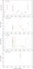 |
Fig. 1 9 Sgr radio fluxes as a function of orbital phase in the 9.1 year period. The detections are shown with their error bars, the upper limits as arrows. Red data points are observations that are centred on 9 Sgr; blue data points have 9 Sgr off-centre. The green bars indicate data that have been combined. Phase 0.0 corresponds to periastron passage. |
3. Radio light curve
We first tried to determine a period from our radio data, using the string-length method (Dworetsky 1983). We normalized the fluxes to their maximum value, so that the flux differences and phase differences have an equal weight. We tried the string-length method with various possibilities: using data at all wavelengths, or only the 6 cm data (most of our data are at 6 cm), including the observations where 9 Sgr was off-centre, or not. No combination, however, leads to a period near that of the spectroscopically determined one. As the quality of the spectroscopic data is much better than the radio data we have, from here on we use the 9.1 year period determined by Rauw (2013, priv. comm.); this value updates the one given by Rauw et al. (2012).
Figure 1 plots the observed radio fluxes at 2, 3.6, 6, and 20 cm as a function of phase in the 9.1 year orbit. The 2 cm fluxes clearly show variability: around periastron (±0.2 in phase) the fluxes are high (around 3 mJy), but in the phases in between the fluxes are only 1–2 mJy. For 6 cm, observations centred on 9 Sgr at periastron are lacking. Based on the off-centre data (which are less reliable), there is a suggestion that the fluxes around periastron are high. Away from periastron the fluxes are consistently low (about 2 mJy). For 3.6 cm, the picture is less clear: there is also variability, but there is no clear indication of a flux increase near periastron. For 20 cm, the only high flux value is quite some distance away from periastron, and it is surrounded on each side by a lower-flux observation. Other wavelengths (0.7 and 90 cm) have only a single observation with a high upper limit.
The 2 cm behaviour is qualitatively in agreement with that expected for an eccentric long-period binary. At all orbital phases the stellar winds collide, leading to the generation of synchrotron emission. As the system approaches periastron, the stars move much closer together, leading to a more energetic collision and therefore more synchrotron emission. In principle, this synchrotron emission could be partially or completely absorbed by the free-free absorption of the material in the stellar winds. However, because of the long period of this system, the stars will be far apart and we would therefore expect little effect of the stellar wind absorption. For a first estimate of the effect we can make use of the effective radii listed in Table 2: these give an indication of the extent of the radio photospheres. We see that for the shorter wavelengths, even at periastron (where the separation between the stars is ~1300 R⊙) the CWR is outside the radio photospheres of each of the stars. Therefore, no significant absorption of the synchrotron photons occurs.
Away from periastron, the spectral index is nearly flat, or slightly negative. The fluxes at all wavelengths are of the order of 2 mJy, slightly lower at 2 cm and somewhat higher at 20 cm. This indicates that we are seeing the non-thermally emitting CWR during a large part of the orbit. It is therefore not completely hidden part of the time, as was the case during the periastron passage of Cyg OB2 # 9 (Blomme et al. 2013). As mentioned above, this can be attributed to the longer period of 9 Sgr, resulting in a CWR region that stays out of the free-free region of each star.
The contribution of the thermal free-free emission of the stellar winds of both stars is negligible. Using the equations of Wright & Barlow (1975) we can calculate the expected thermal radio flux, using the parameters listed in Table 2. The combined flux of both binary components is 0.02 mJy at 2 cm and 0.005 mJy at 20 cm, which is much smaller than the observed fluxes.
Parameters of 9 Sgr used in this study.
4. Modelling
To model the radio-light curve, we basically use the same simple model as presented by Blomme et al. (2013). The use of such a simple model avoids the introduction of less well-known quantities, such as the shock strength, the local magnetic field and the efficiency of the Fermi mechanism.
One of the simplifications in the model is that it assumes a simple shape for the CWR. This is more consistent with a CWR in the adiabatic regime than a radiative one where the instabilities create a lot of structure (Stevens et al. 1992; Pittard 2009). That the CWR of 9 Sgr stays in the adiabatic regime can be seen by comparing the cooling time (tcool) to the escape time (tesc), using the equation from Stevens et al. (1992), 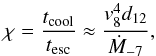 (1)with v8 the wind velocity in units of 1000 km s-1, d12 the distance to the contact discontinuity in units of 107 km, and Ṁ-7 the mass-loss rate in units of 10-7 M⊙ yr-1. Using the values from Table 2 and assuming the contact discontinuity to be halfway between the two stars, we find χ ≈ 740−4700, where the range covers the difference between periastron and apastron values. The high χ values indicate that the collision is indeed adiabatic (see also Rauw et al. 2012).
In the model, we solve the radiative transfer in a three-dimensional grid. For each phase in the orbit, we position the stars in this grid taking into account the orbital parameters and the estimated inclination (Table 2). For a large part of the grid, the volume is filled with wind material coming from the star that is closer. This wind material will contribute to the radio flux through the free-free emission (but we expect the contribution to be small; see Sect. 3). The density at any point in the model is derived from the mass-loss rate and terminal velocity (Table 2). We caution that these two quantities are not well known. The spectral classification of both components is hampered by the fact that the He ii lines cannot be adequately disentangled (Rauw et al. 2012). This classification is then used to determine the mass-loss rate and terminal velocity from the Martins et al. (2005) calibration. Furthermore, any given spectral type/luminosity class corresponds to a range of effective temperature and luminosity rather than the unique values given by the Martins et al. calibration (Weidner & Vink 2010). This turned out to be an important effect in our analysis of Cyg OB2 #9 (Blomme et al. 2013).
For material inside the CWR, we multiply the density by a factor of 4 to take into account the compression in the shocks. The wind material is assumed to be at T = 20 000 K, i.e. just below half of the effective temperature of the stars. A higher temperature is assigned to the material inside the CWR (see below). The grid is 100 000 R⊙ on each side and is centred on the centre of gravity of the binary system.
For the shape of the CWR, we considered two options. The first is as presented in Blomme et al. (2013): the region has the shape of a cone, rotationally symmetric around the line connecting the two stars. The position of this cone and its opening angle are derived from Eichler & Usov (1993, their Eqs. (1) and (3)). The cone is also given a finite thickness which remains constant in the whole simulation volume (Blomme et al., their Fig. 3). Hydrodynamical simulations of adiabatic wind collisions (e.g. Lamberts et al. 2011, their Fig. 4) show a different shape. In these calculations, the CWR is thin near the apex (on the line connecting the two stars) and flares out as we move away from that line. We therefore also considered a second option, where the cone has a half flaring angle (α) instead of a finite thickness (see Fig. 2). For both options, we limit the size of the CWR. Eichler & Usov (1993) estimate the size to be π times the distance from the apex to the star with the weaker wind. In our model, we assume that the size (denoted RCWR) scales proportionally to the distance between the two stars (D), with the scaling factor a free parameter.
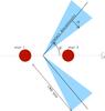 |
Fig. 2 Schematic view of the second option for our model of the CWR. At any given phase, the shape of the CWR (shaded in light-blue) is a cone that is rotationally symmetric around the axis connecting the two stars. It has a half opening angle θ, a half flaring angle α and a size (RCWR) which scales with the separation (D) between the two components. |
Because the material inside the CWR is hot and compressed it will also contribute to the radio flux through free-free emission (Pittard 2010). We therefore need to assign a temperature to this hot material. Rauw et al. (2002) fit the X-ray emission of this system with a multi-temperature thermal model with components at kT = 0.25–0.26 keV, 0.67–0.73 keV, and possibly >1.46 keV. This corresponds to temperatures of 3 × 10⁶, 8 × 10⁶, and 2 × 10⁷ K respectively. In the models we typically run, we calculate the emission measure for the CWR material as 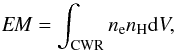 (2)where ne is the electron number density and nH is the proton number density. The integration is over the whole volume of the CWR, and gives a ranges of values of log EM ≈ 55.2−57.2 (EM in cm-3). The observed emission measures of the X-ray temperatures are, respectively, log EM = 56.2, 55.5, and 54.7. This leads to an average temperature of the model CWR of 2 × 10⁵−5 × 10⁶ K. To simplify the model, we assign a single temperature of 1.0 × 10⁶ K to the hot CWR material. Because of the high ratio of the cooling time to the escape time, these temperatures will not significantly decrease inside the CWR as we move away from the apex.
Furthermore, we assume that all the material in the CWR also emits synchrotron radiation. The amount emitted is described by its brightness temperature (Tsync), which we consider a free parameter in our model.
The radiative transfer equation is then solved in this 3D grid, following the procedure outlined in Wright & Barlow (1975). We take into account the free-free emission and absorption processes in the stellar winds and CWR, as well as the synchrotron emission in the CWR. We note that the synchrotron brightness temperature does not play a role in the absorption because synchrotron self-absorption has little effect at GHz frequencies (Pittard et al. 2006). We use an adaptive grid scheme, which refines the grid only in those places where needed to get the required precision in specific intensity and flux.
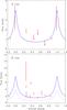 |
Fig. 3 Comparison between 9 Sgr observed and model radio fluxes, as a function of orbital phase in the 9.1 year period. Top: 2 cm fluxes, bottom: 6 cm fluxes. The observed data are plotted in red, the theoretical fluxes of the best-fit model in blue. In the bottom panel, the dotted blue line shows the best-fit 2 cm model applied to the 6 cm data. |
5. Results and discussion
We started by fitting the 2 cm radio light curve, because at this wavelength we see the clearest evidence of phase-locked variability (see Fig. 1). For the observed light curve we used the fluxes from the combined data (see Sect. 2) instead of the separate data, because the combined data have a smaller error bar.
In the model calculations we tried both options for the shape of the CWR, but the more realistic one, where the thickness of the CWR increases as we move away from the apex, gives the better results. We explored the parameter space of the synchrotron brightness temperature (Tsync), half flaring angle (α), and size of the CWR (RCWR). Formally, the best-fit parameters are Tsync = 4.0 × 10⁸ K, α = 40°, and RCWR = 2.0 D; this solution is shown in Fig. 3 (top panel, solid blue line). The result is not unique, however. It is quite insensitive to the size of the CWR. Also, other combinations of Tsync and α can give an almost equally good fit. Our calculations show that this is the case when the combination Tsyncα0.8 has the same value as our formal best fit. Values for the half flaring angle larger than 40° were not explored, as this would make the size of the CWR hydrodynamically unlikely.
The agreement of the theoretical curve with the observed fluxes is good. We correctly predict an increase in the 2 cm flux around periastron (up to ~4 mJy) and a roughly constant flux away from periastron (at the ~1 mJy level). The only discrepant point is at phase 0.25. This indicates that the light curve around periastron is not as symmetric as suggested by the theoretical calculations: the higher flux level extends for a longer time after periastron passage than before it.
We explored the contribution of the various emission and absorption processes to this theoretical light curve by manipulating the temperature and density enhancement in the CWR. If we switch off the synchrotron emission and the density enhancement in the CWR, and set the CWR temperature equal to the wind temperature, we find the free-free contribution of the stellar winds. This turns out to be 0.020 mJy, in good agreement with the values listed in Table 2. By switching off only the synchrotron emission, we find the combined free-free contribution of the stellar winds and the CWR to be 0.021–0.027 mJy (depending on orbital phase). The free-free emission of the CWR is therefore very small. Finally, switching off the free-free absorption in the stellar wind changes the fluxes by only a few percent. The 2 cm radio light curve in Fig. 3 is therefore almost exclusively due to synchrotron emission.
Free-free absorption in the CWR does play an important role, as can be seen from the following argument. An object with a brightness temperature Tsync = 4.0 × 10⁸ K at a distance d = 1.79 kpc with a size equal to the separation between the two components (D = 3011/sin(45°) R⊙) has a flux of 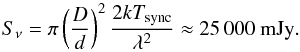 (3)This is clearly more than the 1–4 mJy from the model calculation, hence a large amount of the synchrotron flux must be absorbed in the CWR.
The model used here has a number of simplifying assumptions. One is that the synchrotron brightness temperature is the same for all phases in the orbit. The synchrotron emission is, however, proportional to the number of relativistic electrons (Rybicki & Lightman 1986, Chap. 6). We therefore also tried models with a synchrotron brightness temperature that is proportional to the local electron density. This assumes that the fraction of electrons that becomes relativistic is the same at all phases of the orbit. These models result in a much higher contrast between the maximum and minimum flux, and are therefore not a good fit to the 2 cm observations.
We next applied the same model to the 6 cm fluxes. This is shown by the dotted blue line in the bottom panel of Fig. 3. The model clearly underestimates the observed fluxes. This is not surprising as the synchrotron brightness temperature need not be the same for 6 cm as for 2 cm. In a more detailed synchrotron emission model (such as the one used by Blomme et al. 2010) we would, in principle, be able to calculate the synchrotron brightness temperature for all wavelengths. We note, however, that the Blomme et al. model was not able to explain the observed spectral index of Cyg OB2 #8A, a quantity which is directly related to the relative synchrotron brightness temperatures.
We therefore again considered the synchrotron brightness temperature to be a free parameter and tried to fit the 6 cm observations. We kept the flaring angle and CWR size at their 2 cm best-fit values. The best-fit result is shown by the full blue line in Fig. 3 (bottom panel) and has a brightness temperature of Tsync = 8.0 × 10⁸ K. Away from periastron we obtain the ~2 mJy level, as observed. We have no 6 cm observations around periastron itself, so we cannot judge if the flux maximum has the correct value. The most discrepant point in the fit is what happens around phase 0.25 where we have two observations that are seemingly in contradiction: one at 9.0 ± 2.7 mJy and one at 2.4 ± 0.9 mJy. These flux determinations do not suffer from the measurement problems caused by the nearby Hourglass nebula (Sect. 2). They were taken in VLA configurations that have medium to high spatial resolution, where the effect of the Hourglass nebula is small. We note, however, that both have large error bars, so these detection are only at the ~3σ level. Also for the 6 cm light curve, the parameters are not well determined and other combinations give fits of a similar quality.
The 9 Sgr system is exceptional among the O-type non-thermal radio emitters in that it is the one with the longest period among those that have had their spectroscopic orbit determined. The Cyg OB2 # 8A binary has a substantially shorter period (21.9 d). While one might expect that in such a short-period binary all synchrotron emission would be absorbed by the stellar winds, it turns out that this is still a non-thermal radio emitter (De Becker et al. 2004; Blomme et al. 2010). The systems HD 168112 (P = 1.4 yr, Blomme et al. 2005) and Cyg OB2 #9 (P = 2.35 yr, Nazé et al. 2008, 2012; Van Loo et al. 2008; Blomme et al. 2013) are longer-period binaries with clear non-thermal emission. For Cyg OB2 #9 we know that the CWR is radiative at least during some part of the orbit. This complicates the modelling of the emission. Furthermore, with these periods the effect of orbital motion that turns the CWR into a spiral shape will be important (e.g. Pittard 2009).
There are other O-type non-thermal radio emitters that have longer periods. The Cyg OB2 #5 system is a 6.6 d spectroscopic binary, but the 6.7 yr period in the radio fluxes indicates the presence of a third companion. Furthermore, a CWR is visible at radio wavelengths between Cyg OB2 #5 and a nearby B-type star, implying that Cyg OB2 #5 could be a quadruple system (Kennedy et al. 2010; Dzib et al. 2013). From spectroscopy we know that HD 167971 is a 3.3 d binary, with a third component which may or may not be gravitationally bound (Leitherer et al. 1987). Radio data do not show the 3.3 d period, but reveal a period of ~20 yr, or longer, suggesting that this is due to the CWR between the binary and the third component (Blomme et al. 2007).
What makes 9 Sgr an excellent candidate for modelling studies is that it has an adiabatic wind collision and that it is much less influenced by orbital motion. Longer-period systems (such as Cyg OB2 #5 and HD 167971) might be even better, but they lack the spectroscopic orbital information. A disadvantage of 9 Sgr is that the radio coverage of the orbit, especially at periastron, is somewhat lacking. It should, however, be easy to remedy that situation thanks to the recent upgrade of radio telescopes such as the Karl G. Jansky Very Large Array (JVLA).
6. Conclusions
Using archive data from the VLA that cover a time range of 24 years, we determined the radio light curve of the massive O-type binary 9 Sgr. The presence of the nearby Hourglass nebula, a strong radio source, seriously hampers the detection of 9 Sgr when the VLA is in one of its configurations with lower spatial resolution. The quality of the radio light curve is therefore less than that of other systems studied in this series of papers.
Despite these problems, the 2 cm light curve shows clear phase-locked variability with the 9.1 yr orbit of this system. Fluxes are higher around periastron, as expected, because in this highly eccentric system the wind-wind collision is much stronger (i.e. has a higher ram pressure) when the stars are closer to each other. The 6 cm light curve seems to follow a similar trend, although observations at the periastron passage are missing. The few data we have at 20 cm are more puzzling, as they seem to show large variations at other phases than periastron. The spectral index is approximately zero, and even outside the periastron phases the fluxes are so high that almost all of the emission can be ascribed to synchrotron radiation in the CWR.
A simple model provides a good fit to the 2 cm observations, and allows us to estimate that the synchrotron brightness temperature of the CWR is at least 4 × 10⁸ K. Higher values of the brightness temperature are also possible, provided the flaring angle is smaller. The geometric extent of the CWR is not well constrained in this fitting procedure. We caution that this simple model lacks many important ingredients, such as the hydrodynamics of the CWR, the efficiency with which the electrons get accelerated up to relativistic speeds, the local magnetic field, and the quenching due to the Razin effect.
We propose that 9 Sgr is an ideal candidate for more detailed modelling of its radio emission. Its orbital parameters are sufficiently well known. It has a long period and because of the larger distance between the two components the collision region remains adiabatic during the whole orbit. The effect of orbital motion on the shape of the CWR is also much smaller than in other binary systems. All this simplifies the hydrodynamical part of the modelling. Observationally, the coverage of the orbit should be improved, especially around periastron. This should be quite feasible using recently upgraded radio telescopes such as the JVLA.
Online material
Appendix A: Data table
9 Sgr VLA data.
The spectral index is the quantity α in Fν ∝ να.
Acknowledgments
We thank Gregor Rauw for providing updated values for the orbital parameters and Joan Vandekerckhove for his help with the reduction of the VLA data. We are grateful to the original observers of the VLA archive data used in this paper. D. Volpi acknowledges funding by the Belgian Federal Science Policy Office (Belspo), under contract MO/33/024. This research has made use of the SIMBAD database, operated at the CDS, Strasbourg, France and NASA’s Astrophysics Data System Abstract Service.
References
- Abbott, D. C., Bieging, J. H., Churchwell, E., & Cassinelli, J. P. 1980, ApJ, 238, 196 [NASA ADS] [CrossRef] [Google Scholar]
- Abbott, D. C., Bieging, J. H., & Churchwell, E. 1981, ApJ, 250, 645 [NASA ADS] [CrossRef] [Google Scholar]
- Abbott, D. C., Bieging, J. H., & Churchwell, E. 1984, ApJ, 280, 671 [NASA ADS] [CrossRef] [Google Scholar]
- Bieging, J. H., Abbott, D. C., & Churchwell, E. B. 1989, ApJ, 340, 518 [NASA ADS] [CrossRef] [Google Scholar]
- Blomme, R., Van Loo, S., De Becker, M., et al. 2005, A&A, 436, 1033 [NASA ADS] [CrossRef] [EDP Sciences] [Google Scholar]
- Blomme, R., De Becker, M., Runacres, M. C., van Loo, S., & SetiaGunawan, D. Y. A. 2007, A&A, 464, 701 [NASA ADS] [CrossRef] [EDP Sciences] [Google Scholar]
- Blomme, R., De Becker, M., Volpi, D., & Rauw, G. 2010, A&A, 519, A111 [NASA ADS] [CrossRef] [EDP Sciences] [Google Scholar]
- Blomme, R., Nazé, Y., Volpi, D., et al. 2013, A&A, 550, A90 [NASA ADS] [CrossRef] [EDP Sciences] [Google Scholar]
- Bridle, A. H., & Schwab, F. R. 1999, in Synthesis Imaging in Radio Astronomy II, eds. G. B. Taylor, C. L. Carilli, & R. A. Perley, ASP Conf. Ser., 180, 371 [Google Scholar]
- De Becker, M., Rauw, G., & Manfroid, J. 2004, A&A, 424, L39 [NASA ADS] [CrossRef] [EDP Sciences] [Google Scholar]
- Dworetsky, M. M. 1983, MNRAS, 203, 917 [NASA ADS] [Google Scholar]
- Dzib, S. A., Rodríguez, L. F., Loinard, L., et al. 2013, ApJ, 763, 139 [NASA ADS] [CrossRef] [Google Scholar]
- Eichler, D., & Usov, V. 1993, ApJ, 402, 271 [NASA ADS] [CrossRef] [Google Scholar]
- Gagné, M., Fehon, G., Savoy, M. R., et al. 2012, in Proceedings of a Scientific Meeting in Honor of Anthony F. J. Moffat, eds. L. Drissen, C. Rubert, N. St-Louis, & A. F. J. Moffat, ASP Conf. Ser., 465, 301 [Google Scholar]
- Kennedy, M., Dougherty, S. M., Fink, A., & Williams, P. M. 2010, ApJ, 709, 632 [NASA ADS] [CrossRef] [Google Scholar]
- Kumar, D. L., & Anandarao, B. G. 2010, MNRAS, 407, 1170 [NASA ADS] [CrossRef] [Google Scholar]
- Lamberts, A., Fromang, S., & Dubus, G. 2011, MNRAS, 418, 2618 [NASA ADS] [CrossRef] [Google Scholar]
- Leitherer, C., Forbes, D., Gilmore, A. C., et al. 1987, A&A, 185, 121 [NASA ADS] [Google Scholar]
- Martins, F., Schaerer, D., & Hillier, D. J. 2005, A&A, 436, 1049 [NASA ADS] [CrossRef] [EDP Sciences] [Google Scholar]
- Nazé, Y., De Becker, M., Rauw, G., & Barbieri, C. 2008, A&A, 483, 543 [NASA ADS] [CrossRef] [EDP Sciences] [Google Scholar]
- Nazé, Y., Mahy, L., Damerdji, Y., et al. 2012, A&A, 546, A37 [NASA ADS] [CrossRef] [EDP Sciences] [Google Scholar]
- Perley, R., & Taylor, G. 2003, VLA Calibrator Manual http://www.vla.nrao.edu/astro/calib/manual/index.shtml [Google Scholar]
- Pittard, J. M. 2009, MNRAS, 396, 1743 [NASA ADS] [CrossRef] [Google Scholar]
- Pittard, J. M. 2010, MNRAS, 403, 1633 [NASA ADS] [CrossRef] [Google Scholar]
- Pittard, J. M., Dougherty, S. M., Coker, R. F., O’Connor, E., & Bolingbroke, N. J. 2006, A&A, 446, 1001 [NASA ADS] [CrossRef] [EDP Sciences] [Google Scholar]
- Rauw, G., Blomme, R., Waldron, W. L., et al. 2002, A&A, 394, 993 [NASA ADS] [CrossRef] [EDP Sciences] [Google Scholar]
- Rauw, G., Sana, H., Gosset, E., et al. 2005, in Proc. Massive Stars and High-Energy Emission in OB Associations, eds. G. Rauw, Y. Nazé, R. Blomme, & E. Gosset, 85 [Google Scholar]
- Rauw, G., Sana, H., Spano, M., et al. 2012, A&A, 542, A95 [NASA ADS] [CrossRef] [EDP Sciences] [Google Scholar]
- Rybicki, G. B., & Lightman, A. P. 1986, Radiative Processes in Astrophysics (New York: Wiley-Interscience) [Google Scholar]
- Stevens, I. R., Blondin, J. M., & Pollock, A. M. T. 1992, ApJ, 386, 265 [NASA ADS] [CrossRef] [Google Scholar]
- Van Loo, S., Runacres, M. C., & Blomme, R. 2006, A&A, 452, 1011 [NASA ADS] [CrossRef] [EDP Sciences] [Google Scholar]
- Van Loo, S., Blomme, R., Dougherty, S. M., & Runacres, M. C. 2008, A&A, 483, 585 [NASA ADS] [CrossRef] [EDP Sciences] [Google Scholar]
- Weidner, C., & Vink, J. S. 2010, A&A, 524, A98 [NASA ADS] [CrossRef] [EDP Sciences] [Google Scholar]
- White, R. L. 1985, ApJ, 289, 698 [NASA ADS] [CrossRef] [Google Scholar]
- Wright, A. E., & Barlow, M. J. 1975, MNRAS, 170, 41 [NASA ADS] [CrossRef] [Google Scholar]
All Tables
All Figures
|
Fig. 1 9 Sgr radio fluxes as a function of orbital phase in the 9.1 year period. The detections are shown with their error bars, the upper limits as arrows. Red data points are observations that are centred on 9 Sgr; blue data points have 9 Sgr off-centre. The green bars indicate data that have been combined. Phase 0.0 corresponds to periastron passage. |
| In the text | |
|
Fig. 2 Schematic view of the second option for our model of the CWR. At any given phase, the shape of the CWR (shaded in light-blue) is a cone that is rotationally symmetric around the axis connecting the two stars. It has a half opening angle θ, a half flaring angle α and a size (RCWR) which scales with the separation (D) between the two components. |
| In the text | |
|
Fig. 3 Comparison between 9 Sgr observed and model radio fluxes, as a function of orbital phase in the 9.1 year period. Top: 2 cm fluxes, bottom: 6 cm fluxes. The observed data are plotted in red, the theoretical fluxes of the best-fit model in blue. In the bottom panel, the dotted blue line shows the best-fit 2 cm model applied to the 6 cm data. |
| In the text | |
Current usage metrics show cumulative count of Article Views (full-text article views including HTML views, PDF and ePub downloads, according to the available data) and Abstracts Views on Vision4Press platform.
Data correspond to usage on the plateform after 2015. The current usage metrics is available 48-96 hours after online publication and is updated daily on week days.
Initial download of the metrics may take a while.