© ESO, 2014

1. Introduction

Our Galaxy is full of interstellar medium (ISM), such as gas and dust grains (Draine 2003), which are produced by the nuclear burning within the stars and blown out by supernova explosions and stellar winds. The absorption and scattering of the starlight emitted from distant objects by the dust grains leads to the Galactic interstellar extinction, which varies with directions depending of the different composition of the dusts in the interstellar space. The interstellar extinction is also referred to as the reddening, or the color excess, because the tendency of the absorption and scattering is much larger in the blue than in the red wavelength. The extinction as a function of the wavelength is related to the size distribution and abundances of the grains. Therefore, it plays an important role in understanding the nature of the interstellar medium.

The flux of extragalactic objects, such as galaxies, quasars, etc., suffers different extinction in different bands. This effect leads to some bias on the extragalactic studies (Guy et al. 2010; Ross et al. 2011; Fang et al. 2011; Tian et al. 2011). Therefore, understanding the total interstellar extinction in every line of sight (LoS) is crucial for accurate flux measurements. The all-sky dust map can either be constrained by measuring interstellar extinction, or constrained by employing a tracer as ISM, e.g., HI. One of the most broadly used dust maps was published by Schlegel et al. (1998, hereafter SFD), which was derived from observations of dust emission at 100 μm and 240 μm with an angular resolution at about 6 arcmin. Since then, many other works have claimed discrepancy with their results. Stanek (1998) inferred that SFD overestimated the extinction in some large extinction regions from the study of the globular clusters. Arce & Goodman (1999) argued that the SFD dust map overestimated by 20–40% in Taurus region from star counts, colors, etc. Dobashi et al. (2005) studied the optical star counts and concluded that SFD overestimated the extinction value by at least a factor of two. Peek & Graves (2010) independently estimated the extinction using the standard galaxies and their result is consistent with the SFD map in most of the area within the uncertainty of 3 mmag in E(B − V), though some regions do deviate from SFD by up to 50%. Schlafly et al. (2010), Schlafly & Finkbeiner (2011), and Yuan et al. (2013) use the blue tip of Sloan Digital Sky Survey (SDSS) stellar locus, SDSS stellar spectra , and multiple passbands from several photometric imaging surveys respectively to measure the reddening and claim SFD overestimates E(B − V) by about 14%. However, Berry et al. (2011) argues that the overestimation only exists in the southern sky, while the dust map at high northern Galactic latitudes looks good.

In this work, we use the blue horizontal branch (BHB) stars to map the total interstellar extinction over the northern Galactic cap covered by the SDSS survey. The BHB stars are luminous and far behind the dust disk, which contribute to most of the interstellar extinction. Thanks to the five-band high accuracy photometry provided by SDSS, the BHB stars are available to derive the reddening in multiple color indexes which allows us to estimate the extinction law, or R_V, simultaneously.

The outline of this paper is as follows. In Sect. 2, we describe the Bayesian method for the estimation of the total extinction via BHB stars and the estimation of the mean R_V and A_V in the given LoS. In Sect. 3, we assess the performance of the Bayesian method for the total extinction, and validate the method to estimate the R_V. In Sect. 4, we describe the criteria to select the BHB sample. We selected a total of 12 530 BHB stars with these criteria, covering most of SDSS footprint. The result of the color excess in four color indexes and the comparisons with other works are presented and discussed in Sect. 5. In the last section, we draw the conclusions.

2. Method

2.1. Bayesian method for color excess

The total Galactic extinction in a given LoS is measured from the offset of the measured color indexes of the BHB stars from their intrinsic color. A set of BHB stars, whose dereddened color index, { c_k } (where k = 1,2,...,N_BHB), is around their intrinsic color index, are selected as template stars. The reddening of a field BHB stars can then be estimated by comparing measured colors with the templates. Given a LoS i with N_i field BHB stars, the posterior probability of the reddening E_i is denoted as p(E_i |  { ĉ_ij } , { c_k }), where ĉ_ij is the observed color index vector of the BHB star j in the LoS i, and c_k is the intrinsic color index vector of the template BHB star k. According to the Bayes theorem, this probability can be written as $\mathit{p}\mathrm{\left(}{{E}}_{\mathit{i}}\mathrm{\right|}\mathrm{\left\{}{{ĉ}}_{\mathit{ij}}\mathrm{\right\}}\mathit{,}\mathrm{\left\{}{{c}}_{\mathit{k}}\mathrm{\right\}}\mathrm{)}\mathrm{=}{p}\mathrm{(}\mathrm{\left\{}{{ĉ}}_{\mathit{ij}}\mathrm{\right\}}\mathrm{\left|}{{E}}_{\mathit{i}}\mathit{,}\mathrm{\right\{}{{c}}_{\mathit{k}}\mathrm{\left\}}\mathrm{\right)}{P}\mathrm{\left(}{{E}}_{\mathit{i}}\mathrm{\right|}\mathrm{\left\{}{{c}}_{\mathit{k}}\mathrm{\right\}}\mathrm{)}\mathit{.}$(1)Since E_i is independent of the template BHB stars’ { c_k }, the prior P(E_i |  { c_k }) is equivalent to P(E_i), which is assumed to be flat in this work. The right-hand side of Eq. (1) can now be rewritten as 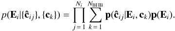$\begin{array}{ccc}\mathit{p}\mathrm{\left(}{{E}}_{\mathit{i}}\mathrm{\right|}\mathrm{\left\{}{{ĉ}}_{\mathit{ij}}\mathrm{\right\}}\mathit{,}\mathrm{\left\{}{{c}}_{\mathit{k}}\mathrm{\right\}}\mathrm{)}\mathrm{=}\underset{\mathit{j}\hspace{0.17em}\mathrm{=}\hspace{0.17em}\mathrm{1}}{\overset{{\mathit{N}}_{\mathit{i}}}{\mathrm{􏽙}}}\sum _{\mathit{k}\hspace{0.17em}\mathrm{=}\hspace{0.17em}\mathrm{1}}^{{\mathit{N}}_{\mathrm{BHB}}}{p}\mathrm{(}{{ĉ}}_{\mathit{ij}}\mathrm{\left|}{{E}}_{\mathit{i}}\mathit{,}{{c}}_{\mathit{k}}\mathrm{\right)}{p}\mathrm{\left(}{{E}}_{\mathit{i}}\mathrm{\right)}\mathit{.}& & \end{array}$(2)We assume that the likelihood p(ĉ_ij | (E_i,c_k)) is a multivariate Gaussian and so can be expressed as: 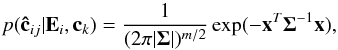$\mathit{p}\mathrm{\left(}{{ĉ}}_{\mathit{ij}}\mathrm{\right|}{{E}}_{\mathit{i}}\mathit{,}{{c}}_{\mathit{k}}\mathrm{)}\mathrm{=}\frac{\mathrm{1}}{\mathrm{\left(}\mathrm{2}\mathit{\pi }\mathrm{\right|}{\Sigma }\mathrm{|}{\mathrm{)}}^{\mathit{m}\mathit{/}\mathrm{2}}}\exp \mathrm{(}\mathrm{-}{{x}}^{\mathit{T}}{{\Sigma }}^{-1}{x}\mathrm{)}\mathit{,}$(3)where x = E + c_k − ĉ_ij, and Σ is the mth rank covariance matrix of the measurement of the color indexes of the star j; Σ is composed of the measurement error ${\Sigma }\mathrm{=}\left[\begin{array}{c}\\ {\mathit{\sigma }}_{\mathit{u}}^{\mathrm{2}}\mathrm{+}{\mathit{\sigma }}_{\mathit{g}}^{\mathrm{2}}& \mathrm{-}{\mathit{\sigma }}_{\mathit{g}}^{\mathrm{2}}& \mathrm{0}& \mathrm{0}\\ \mathrm{-}{\mathit{\sigma }}_{\mathit{g}}^{\mathrm{2}}& {\mathit{\sigma }}_{\mathit{g}}^{\mathrm{2}}\mathrm{+}{\mathit{\sigma }}_{\mathit{r}}^{\mathrm{2}}& \mathrm{-}{\mathit{\sigma }}_{\mathit{r}}^{\mathrm{2}}& \mathrm{0}\\ \mathrm{0}& \mathrm{-}{\mathit{\sigma }}_{\mathit{r}}^{\mathrm{2}}& {\mathit{\sigma }}_{\mathit{r}}^{\mathrm{2}}\mathrm{+}{\mathit{\sigma }}_{\mathit{i}}^{\mathrm{2}}& \mathrm{-}{\mathit{\sigma }}_{\mathit{i}}^{\mathrm{2}}\\ \mathrm{0}& \mathrm{0}& \mathrm{-}{\mathit{\sigma }}_{\mathit{i}}^{\mathrm{2}}& {\mathit{\sigma }}_{\mathit{i}}^{\mathrm{2}}\mathrm{+}{\mathit{\sigma }}_{\mathit{z}}^{\mathrm{2}}\end{array}\right]\mathit{,}$(4)where the σ_u, σ_g, σ_r, σ_i, and σ_z are the uncertainties of magnitudes in the u, g, r, i, and z bands, respectively.

2.2. R_V and A_V

After deriving the probability of the reddening in a LoS, the most likely reddening values, ${\mathit{E}}_{\mathit{i}}\mathrm{=}\mathrm{\left(}\mathit{E}\mathrm{\right(}\mathit{u}\mathrm{-}\mathit{g}\mathrm{\left)}\mathit{,E}\mathrm{\right(}\mathit{g}\mathrm{-}\mathit{r}\mathrm{\left)}\mathit{,E}\mathrm{\right(}\mathit{r}\mathrm{-}\mathit{i}\mathrm{\left)}\mathit{,E}\mathrm{\right(}\mathit{i}\mathrm{-}\mathit{z}\mathrm{\left)}\mathrm{\right)}\mathit{,}$(5)can be obtained from the probability density function (PDF). They can be used to derive the R_V and A_V given an extinction model, such as the one in Cardelli et al. (1989, hereafter CCM), $\begin{array}{ccc}\mathit{E}\mathrm{(}\mathit{u}\mathrm{-}\mathit{g}\mathrm{)}\mathrm{=}\left(\left({\mathit{a}}_{\mathit{u}}\mathrm{+}\frac{{\mathit{b}}_{\mathit{u}}}{{\mathit{R}}_{\mathit{V}}}\right)\mathrm{-}\left({\mathit{a}}_{\mathit{g}}\mathrm{+}\frac{{\mathit{b}}_{\mathit{g}}}{{\mathit{R}}_{\mathit{V}}}\right)\right)\mathrm{\ast }{\mathit{A}}_{\mathit{V}}& & \\ \mathit{E}\mathrm{(}\mathit{g}\mathrm{-}\mathit{r}\mathrm{)}\mathrm{=}\left(\left({\mathit{a}}_{\mathit{g}}\mathrm{+}\frac{{\mathit{b}}_{\mathit{g}}}{{\mathit{R}}_{\mathit{V}}}\right)\mathrm{-}\left({\mathit{a}}_{\mathit{r}}\mathrm{+}\frac{{\mathit{b}}_{\mathit{r}}}{{\mathit{R}}_{\mathit{V}}}\right)\right)\mathrm{\ast }{\mathit{A}}_{\mathit{V}}& & \\ \mathit{E}\mathrm{(}\mathit{r}\mathrm{-}\mathit{i}\mathrm{)}\mathrm{=}\left(\left({\mathit{a}}_{\mathit{r}}\mathrm{+}\frac{{\mathit{b}}_{\mathit{r}}}{{\mathit{R}}_{\mathit{V}}}\right)\mathrm{-}\left({\mathit{a}}_{\mathit{i}}\mathrm{+}\frac{{\mathit{b}}_{\mathit{i}}}{{\mathit{R}}_{\mathit{V}}}\right)\right)\mathrm{\ast }{\mathit{A}}_{\mathit{V}}& & \\ \mathit{E}\mathrm{(}\mathit{i}\mathrm{-}\mathit{z}\mathrm{)}\mathrm{=}\left(\left({\mathit{a}}_{\mathit{i}}\mathrm{+}\frac{{\mathit{b}}_{\mathit{i}}}{{\mathit{R}}_{\mathit{V}}}\right)\mathrm{-}\left({\mathit{a}}_{\mathit{z}}\mathrm{+}\frac{{\mathit{b}}_{\mathit{z}}}{{\mathit{R}}_{\mathit{V}}}\right)\right)\mathrm{\ast }{\mathit{A}}_{\mathit{V}}\mathit{.}& & \end{array}$(6)These are linear equations for A_V and A_V/R_V and can be easily solved with a least-squares or χ² method to find the values of A_V and R_V for each BHB star. The A_V and R_V values in each LoS are obtained by the median value of all the BHB stars located in each LoS; the errors can be estimated by the median absolute deviation. For the wavelength of the five bands (u, g, r, i, and z) in SDSS, we adopt 3551 Å, 4686 Å, 6165 Å, 7481 Å, and 8931 Å as their effective wavelengths, respectively (Fukugita et al. 1996; Stoughton et al. 2002), a_x and b_x are calculated based on CCM.

2.3. Template BHB stars

To estimate the total extinction for a given LoS, we need to find a set of BHB samples as the template, i.e., those having accurate color indexes without extinction. Metal-poor globular clusters are good sample for extracting this kind of template BHB stars. There are seven globular clusters covered by SDSS in the northern Galactic cap. Their basic parameters, distance (R_sun), metallicity ([Fe/H]), color excess (E(B − V)), etc., are selected from the literature (Harris 1996, 2010 edition). We cross-identify the stars located within radius of 30 arcmin around the globular clusters with the BHB catalogue (Harris 1996, 2010 edition). Then we remove the field stars whose magnitudes in the g band are different by more than 0.5 mag from the corresponding g-band magnitude of the horizontal branch of a globular clusters. Finally, 94 BHB stars are remained. We validated the 94 template stars according to their distances calculated using Eq. (5) in Fermani & Schönrich (2013) with the known metallicity and the g − r of each globular cluster (Harris 1996, 2010 edition). A BHB star whose distance is different by more than 5 kpc from the corresponding globular cluster is probably not located in this globular cluster. According to this criterion, all the 94 BHB stars are within their corresponding globular cluster.

Based on the CCM algorithm, Doug Welch¹ provides an absorption law calculator to determine the total absorption at wavelengths between 0.10 μm and 3.33 μm. Given R_V = 3.1, A_V, and the average wavelength of the u,g,r,i, and z bands, we obtain the total extinction in each band: $\begin{array}{ccc}{\mathit{A}}_{\mathit{u}}& \mathrm{=}& \mathrm{4.896}\mathrm{\ast }\mathit{E}\mathrm{(}\mathit{B}\mathrm{-}\mathit{V}\mathrm{)}\\ {\mathit{A}}_{\mathit{g}}& \mathrm{=}& \mathrm{3.788}\mathrm{\ast }\mathit{E}\mathrm{(}\mathit{B}\mathrm{-}\mathit{V}\mathrm{)}\\ {\mathit{A}}_{\mathit{r}}& \mathrm{=}& \mathrm{2.728}\mathrm{\ast }\mathit{E}\mathrm{(}\mathit{B}\mathrm{-}\mathit{V}\mathrm{)}\\ {\mathit{A}}_{\mathit{i}}& \mathrm{=}& \mathrm{2.093}\mathrm{\ast }\mathit{E}\mathrm{(}\mathit{B}\mathrm{-}\mathit{V}\mathrm{)}\\ {\mathit{A}}_{\mathit{z}}& \mathrm{=}& \mathrm{1.503}\mathrm{\ast }\mathit{E}\mathrm{(}\mathit{B}\mathrm{-}\mathit{V}\mathrm{)}\mathit{.}\end{array}$(7)The reddening in each color can now be obtained by $\begin{array}{ccc}\mathit{E}\mathrm{(}\mathit{u}\mathrm{-}\mathit{g}\mathrm{)}& \mathrm{=}& {\mathit{A}}_{\mathit{u}}\mathrm{-}{\mathit{A}}_{\mathit{g}}\\ \mathit{E}\mathrm{(}\mathit{g}\mathrm{-}\mathit{r}\mathrm{)}& \mathrm{=}& {\mathit{A}}_{\mathit{g}}\mathrm{-}{\mathit{A}}_{\mathit{r}}\\ \mathit{E}\mathrm{(}\mathit{r}\mathrm{-}\mathit{i}\mathrm{)}& \mathrm{=}& {\mathit{A}}_{\mathit{r}}\mathrm{-}{\mathit{A}}_{\mathit{i}}\\ \mathit{E}\mathrm{(}\mathit{i}\mathrm{-}\mathit{z}\mathrm{)}& \mathrm{=}& {\mathit{A}}_{\mathit{i}}\mathrm{-}{\mathit{A}}_{\mathit{z}}\mathit{.}\end{array}$(8)Table 1 provides the basic parameters, including E(B − V), for all the seven globular clusters. Equation (7) is applied to convert the E(B − V) to total extinction in each band. The E(a − b) listed in the table are estimated for the case of R_V = 3.1. Alternative R_V values do not significantly change the reddening of the template stars. For instance, the variation of E(a − b) (a and b are two arbitrary SDSS bands) is less than 5%0 when R_V changes from 2.5 to 4.1. This is because the E(B − V) for the clusters are very small and the difference in the reddening due to the variate extinction law is negligible owing to the accuracy of the photometry in SDSS. The intrinsic colors of the template BHB stars is then obtained by subtracting the small reddening in each color.

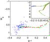Fig. 1 The 94 dereddened BHB stars and two typical isochrones in the color vs. absolute magnitude plane. The blue points are the BHB stars, the green curve is the isochrone with metallicity of − 2.28 dex and age of 13.5 Gyrs. And the red curve is another isochrone with metallicity − 2.0 at the same age. Both isochrones are obtained from Girardi et al. (2010).

Figure 1 shows the 94 dereddened BHB stars and two typical isochrones in a color-absolute magnitude diagram. The blue points are the BHB stars. The green and red curves are the isochrones with age 13.5 Gyr and metallicity − 2.28 and − 2.0 dex, respectively² (Girardi et al. 2010). It shows that the observed BHB templates are consistent with the isochrones.

3. Validation of the method

At high Galactic latitudes, the total extinction is usually very small, even smaller than 0.1 mag in E(B − V). Figure 1 shows that the template BHB stars have dispersion up to 0.3 mag in g − r because of the spread in effective temperatures, and so it is important to examine the validity of our method and to assess the performance of the reddening estimation before applying the method to the real data. We ran Monte Carlo simulations based on the template BHB stars. We supposed that each simulation was for one LoS, i.e., all tracers have the same reddening values but different photometric uncertainties in each LoS. For each LoS, we selected a random reddening in the u, g, r, i, and z bands for arbitrarily selected BHB template stars with random Gaussian noises to mimic the uncertainties of the photometry. Specifically, an observed color index in the simulation is obtained by 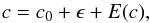$\mathit{c}\mathrm{=}{\mathit{c}}_{\mathrm{0}}\mathrm{+}\mathit{ϵ}\mathrm{+}\mathit{E}\mathrm{\left(}\mathit{c}\mathrm{\right)}\mathit{,}$(9)where c₀ is the noise-free, dereddened color index, e is the random error following a Gaussian with zero mean and σ ∈  [0.02,0.08], and E(c) is the reddening.

In this work we concentrate on the extinction at high Galactic latitudes, and so we only test the low extinction cases. Considering that R_V may be variant with the LoS, we let the extinction curve have a freedom of changing, specifically, the reddening value E(u − g) = E(g − r) + Δ_ug; both the E(g − r) and Δ_ug are arbitary values for each LoS, and E(g − r) ∈  [0,0.14] mag, Δ_ug ∈  [0,0.05]. We arbitrarily selected 10–50 BHB template stars as field stars in each LoS.

We applied the method described in section 2 to the mock stars and ran the Monte Carlo simulations for 900 LoS with different testing samples. One of the simulations is presented in Fig. 2. And Fig. 3 shows the comparison between the estimated and the true extinction values in four colors. Figure 4 shows the histogram of the residuals of the estimated values. It is noted that most of the residuals are less than 0.01 mag, which suggests that the Bayesian method we employed in this work is robust.

To validate the method of the R_V estimation, we initially obtained the E(B − V) values in each LoS from the extinction maps released by SFD. The values of E(u − g) and E(g − r) is estimated according to Eqs. (7) and (8), given R_V = 3.1. We then solve Eq. (6) with the least-squares or χ² method described in Sect. 2.2 to obtain the R_V in each LoS. Figure 5 displays the histogram of R_V distribution; the yellow vertical line marks the location of R_V = 3.1. The peak of R_V distribution is exactly on the yellow line, proving the accurate performance of the method for the R_V estimation.

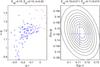Fig. 2 One simulated LoS example of 900 Monte Carlo simulations for validation of the Bayesian method. In the left panel, the blue crosses stand for the 94 template BHB stars; the red points are selected field stars with random reddening values and random Gaussian noises in photometry. The right panel shows the contour of the posterior probability of the reddening E(u − g) and E(g − r) estimated from the Bayesian method. The large blue cross marks the most likely reddening value with a 1σ error.

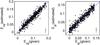Fig. 3 Estimated reddening values vs. the given values in the simulation. The mean 1σ error bars are marked at the bottom.

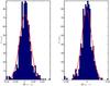Fig. 4 Histogram of the residuals of the estimated reddening values in the simulation. The red curves are the Gaussian fit profiles with σ ≃ 0.01.

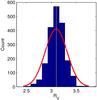Fig. 5 Histogram of estimated RV in the simulation. The red curves are the Gaussian fit profiles with the mean value ⟨ RV ⟩  ≃ 3.1 and σ ≃ 0.16; the yellow line marks the location of RV = 3.1.

4. Data

Sloan Digital Sky Survey has provided an uniform and contiguous imaging of about one third of the sky, mostly at high Galactic latitudes (Aihara et al. 2011). The SDSS imaging is performed nearly simultaneously in the five optical filters: u, g, r, i, and z (Gunn et al. 1998; Fukugita et al. 1996). The images are uniformly reduced by the photometric pipeline, and the completeness of data reduction is around 95% under the limited magnitudes 22.1, 22.4, 22.1, 21.2, and 20.3 for the five bands, respectively.

The BHB sample used in this work was selected from Smith et al. (2010), the authors identified 27 074 BHB stars candidates out of 294 652 stars from SDSS Data Release 7 (DR7) using the support vector machine (SVM) trained by the spectroscopic sample of BHB stars (Xue et al. 2008).

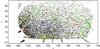Fig. 6 Data sample distribution. The black points are the 13 143 BHB candidates selected in this work. We confirm that these samples are contaminated by at least 76 main-sequence stars (red circles), 311 blue straggler (green points), and 227 other objects (yellow points) (Xue et al. 2008). The seven globular star clusters listed in Table 1 are marked by blue circles.

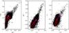Fig. 7 All of the BHB stars used in this work in the color–color space. The tails of the black points are due to the extinction. The red points are the 94 template BHB stars calibrated with the known extinction. The magenta arrows show the reddening direction, the starting point of each arrow is the median value of the color indexes of the 94 template stars, and the terminal is the reddened original point with RV = 3.1 and E(B − V) = 0.1.

Most of the BHB stars in the northern Galactic cap region are more distant than 10 kpc, as shown in the Fig. 19 of Smith et al. (2010). Since the integrated line-of-sight extinction mainly comes from the Galactic gas disk, the typical thickness of the gas disk is far less than 10 kpc; therefore, the distant BHB stars are suitable for the estimation of the total Galactic extinction. In order to trace the extinction in most of the SDSS LoS, we selected a total of 12 530 field BHB stars according to the following criteria:

• g < 19.0, the BHB stars are bright enough, which ensures that i) there is less contamination; and ii) the photometric error is sufficiently small (on average smaller than 0.020 mag in the SDSS bands).

• The sky coverage to 110° < α < 260° and −10° < δ < 70°, where the sky is continuously covered by SDSS DR7.

• (g − r) >  −0.3, according to Yanny et al. (2000).

• P_SVM > 0.5, P_SVM is the BHB probability from the SVM provided by Smith et al. (2010). The average contamination and completeness are about 30–40% and 70–80% when the classification threshold is equal to 0.5, according to Figs. 11 and 12 in Smith et al. (2010).

• Remove the contamination, such as blue stragglers (BS), main-sequence (MS) stars, etc. (as shown in Fig. 6), which have been ambiguously classified by Xue et al. (2008). Even then, most of the contaminations cannot be removed because we do not have the spectra for the entire BHB sample.

Figures 6 and 7 present the selected data distributions in the equatorial coordinate and color–color spaces, respectively.

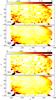Fig. 8 Reddening maps for E(u − g) (top panel) and E(g − r) (bottom panel). The top plots in each panel give the reddening map estimated by the Bayesian method, while the bottom ones show the same map released by SDSS. The blanks and other features in our maps have probably occurred because the reddening values are too small at the high Galactic latitudes to be estimated accurately; the reddening values in these regions are very close to the average of photometric error.

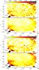Fig. 9 Reddening maps for E(r − i) (top panel) and E(i − z) (bottom panel). The top plots in each panel give the reddening map estimated by the Bayesian method, while the bottom ones show the same map released by SDSS.

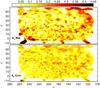Fig. 10 Top panel shows the AV map, while bottom panel shows its error in the same color level; the value of AV is the median AV of all the BHB stars in each LoS, and the error is calculated by the median absolute deviation of AV in each LoS.

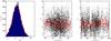Fig. 11 Distribution of the estimated RV is shown in the left panel. The red line shows the best-fit Gaussian with μ ≃ 2.4 and σ ≃ 1.05. The middle and right panels are the estimated RV as functions of Galactic latitude and longitude, respectively. The red curves show the ⟨ RV ⟩, which keeps constant at ~2.5 over all latitudes and longitudes.

5. Analysis and results

The sky is separated into 1° × 1° LoS. The nearest 18 BHB stars around the center of the LoS are involved in the estimation of the reddening. However, at high Galactic latitudes, the BHB stars are too sparse and extend to larger areas. In these LoS, the spatial resolution of the reddening is lower than the average level. Unlike the extinction near the Galactic disk, the extinction is usually very low at high Galactic latitudes and the spatial variation is not intensive. Therefore, we assume that all the reddening values in color bands for the 18 stars are essentially the same. The 18 stars included in each LoS are sufficient for the Bayesian method according to the Monte Carlo simulations; the average error of reddening is about 0.018 if the number of field stars in each LoS is less than 18, which is smaller than the photometric error. In total, we get 9,079 valid LoS.

To obtain the reddening, we calculate the likelihood values at every point in the parameter grid with a step of 0.005 mag. In principle, this simple method is too time-consuming to be used on traditional computational devices, especially in the context of high color dimension. Thanks to the up-to-date GPU computational technique that is programmed on a commercial graphics card containing hundreds of cores, this computation can be simultaneously run with hundreds of threads. This powerful technique allows us to calculate the likelihood in the parameter grid directly. In this work, we use NVIDIA Compute Unified Device Architecture (CUDA) to implement the parallel code in the C++ programming language, and running on the GTX580 card, it only takes several seconds to get the posterior distribution of the reddening value spanned in the 4D color space (e.g. u − g, g − r, r − i, and i − z) for each LoS.

5.1. Reddening map

Figures 8 and 9 present the reddening maps in four colors. The top panels show the results estimated for each color, and the bottom panels are the averaged reddening provided by the SDSS catalogue, that were derived from SFD.

The blue points scattered in Fig. 13 present the differential reddening, ΔE(a − b) = E(a − b)_this − E(a − b)_SDSS (a and b stand for any two bands), at variant Galactic latitudes for the four colors. The green lines mark ΔE(a − b) = 0, and the red lines are the average of reddening values in Galactic latitude bins. The red lines suggest that the averaged extinctions estimated in this work are very close to those released by SDSS; the rms in the four color are 0.029, 0.022, 0.016, and 0.013, which are almost at the same level as the photometric errors of SDSS.

To estimate the R_V, we adopt the CCM model; A_V and R_V are then estimated according to the method described in Sect. 2. Figure 10 shows the filled contour maps of A_V and its error in Galactic coordinates.

The left panel in Fig. 11 shows the histogram of R_V (red curve), which is well fitted by a Gaussian with μ ~ 2.4 and σ ~ 1.05. The middle and right panels are the distribution of R_V at different Galactic latitudes and longitudes, respectively. The red curves show the ⟨ R_V ⟩, which keeps a constant value of ~2.5 at all latitudes and longitudes. It implies that ⟨ R_V ⟩ is invariant with LoS at high Galactic latitudes. Although the measured ⟨ R_V ⟩ is smaller than 3.1, which is frequently used, they are in agreement within 1σ.

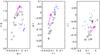Fig. 12 Color–color diagrams of the 18 BHB stars (black circles) on the LoS of (l,b) = (39,50), and 24 contamination stars (blue points) on this LoS, selected from Smith et al. (2010). The magenta arrows present the reddening direction, the starting point of each arrow is the median value of the color indexes of the 18 field stars, and the terminal is the reddened original point with RV = 3.1 and E(B − V) = 0.1.

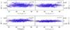Fig. 13 The blue dots are the differences between the estimated reddening in this work and those from SDSS at different Galactic latitudes. The green lines indicate ΔE(a − b) = 0 and the red curves the average values of the differential reddening values in different Galactic latitude bins.

6. Discussion and conclusion

Smith et al. (2010) classifies the BHB and BS stars from their photometry. Thus, the contamination of the BS stars in the BHB catalogue is unavoidable. How do these small fractions of contamination affect the measurement of the extinction?

To investigate the impact of the non-BHB objects, we focus on one LoS selected randomly, for instance, the LoS of (l,b) = (39,50), and calculate the reddening values under the different levels of contamination. We totally get a total of 24 contamination stars in the LoS of (l,b) = (39,50) through the following two steps:

• (1)

  cross-matching the field BHB stars in the selectedLoS with the catalogue provided by Smithet al. (2010), under the error-radiusof 1.0°; and

• (2)

  picking the cross-matched objects with the criteria of g < 19.0, P_SVM < 0.3 and modP < 0.3; these two BHB probabilities are the outputs of two different methods of selecting select BHB candidates (Smith et al. 2010).

Figure 12 shows the color–color diagram of the 24 contamination stars (blue points), with the 18 field BHB stars (black circles); all of these objects are located in the same LoS, the LoS of (l,b) = (39,50). The red arrows present the reddening direction; the starting point of each arrow is the median value of the color indexes of the 18 field stars; and the terminal is the original point after reddening with the parameters of R_V = 3.1 and E(B − V) = 0.1.

We randomly removed 2, 4, or 6 targets from the 18 BHB field stars, and used the same number of contamination stars, selected arbitrarily from the 24 contaminations, to replace the removed BHB stars. Thus, we could get different levels of contaminations ranging from 11% to 33%. Table 2 lists the average of reddening values calculated from 50 BHB samples simulated with the different situations of contamination. The results tell us the reddening in the color of u − g is decreased by the increasing contaminations, and the reddening in the color of g − r is slightly increased, while the reddenings are almost not affacted by the contaminations in both the r − i and i − z color indexes. We also ran the simulations of contamination in other LoS, for example, the LoS of (l,b) = (332,67), and we came to a similar conclusion. The larger E(u − g)/E(g − r) caused by the impact of contamination will give rise to a larger R_V according to Eq. (6).

In this paper, we use BHB stars to estimate the total extinction in the Milky Way. Because the extinction values are very small at high Galactic latitudes, they require accurate photometry and proper estimation methods. The SDSS photometry provides sufficient accuracy up to 2%, allowing us to estimate the reddening to an accurate of 0.01 mag. On the other hand, although the BHB stars are sparsely distributed in an elongated region in color space, the Bayesian statistics works well in the determination of the small value of the reddening. Simulations show that by combining the accurate magnitudes of BHB stars with the Bayesian method, we can determine the reddening values in four colors at high Galactic latitudes.

Figure 13 shows that the average difference between the reddening measured in this work and SFD is around 0.02 mag, which approaches to the limit of the uncertainty of the photometry. Therefore, the extinction map derived from the BHB stars are highly consistent with SFD, although there are some slight differences on small scales.

The R_V inferred from the reddening are centered around 2.4. However, the dispersion of R_V is large. This is partly because the spatial distribution of R_V must not be a single fixed value, but is extended over a range. And the estimation of R_V using very low reddening is crucial and suffers from high uncertainty. Hence, the higher uncertainties eliminate the slight spatial variation of R_V and produce a broad and smooth distribution of the R_V.

Online material

Acknowledgments

The authors thank Biwei Jiang and Jian Gao for the helpful discussions, and thank Jaswant Yadav for reading the manuscript. H.J.T. thanks the support from LAMOST Fellowship (No. Y229041001), the China Postdocatoral Science Foundation grant (No. 2012M520384), and the union grant (No. U1231123, U1331202) of NFSC and CAS. C.L. thanks the support from NSFC grant (No. U1231119), and the 973 Program grant (No. 2014CB845704). X.L.C. thanks the support from the Ministry of Science and Technology 863 Project grant (No. 2012AA121701), the NSFC grant (No. 11073024, 11103027), and the CAS Knowledge Innovation grant (No. KJCX2-EW-W01).

References

All Tables

All Figures

	Fig. 1 The 94 dereddened BHB stars and two typical isochrones in the color vs. absolute magnitude plane. The blue points are the BHB stars, the green curve is the isochrone with metallicity of − 2.28 dex and age of 13.5 Gyrs. And the red curve is another isochrone with metallicity − 2.0 at the same age. Both isochrones are obtained from Girardi et al. (2010).
In the text

Fig. 2 One simulated LoS example of 900 Monte Carlo simulations for validation of the Bayesian method. In the left panel, the blue crosses stand for the 94 template BHB stars; the red points are selected field stars with random reddening values and random Gaussian noises in photometry. The right panel shows the contour of the posterior probability of the reddening E(u − g) and E(g − r) estimated from the Bayesian method. The large blue cross marks the most likely reddening value with a 1σ error.

In the text

	Fig. 3 Estimated reddening values vs. the given values in the simulation. The mean 1σ error bars are marked at the bottom.
In the text

	Fig. 4 Histogram of the residuals of the estimated reddening values in the simulation. The red curves are the Gaussian fit profiles with σ ≃ 0.01.
In the text

	Fig. 5 Histogram of estimated RV in the simulation. The red curves are the Gaussian fit profiles with the mean value ⟨ RV ⟩  ≃ 3.1 and σ ≃ 0.16; the yellow line marks the location of RV = 3.1.
In the text

	Fig. 6 Data sample distribution. The black points are the 13 143 BHB candidates selected in this work. We confirm that these samples are contaminated by at least 76 main-sequence stars (red circles), 311 blue straggler (green points), and 227 other objects (yellow points) (Xue et al. 2008). The seven globular star clusters listed in Table 1 are marked by blue circles.
In the text

Fig. 7 All of the BHB stars used in this work in the color–color space. The tails of the black points are due to the extinction. The red points are the 94 template BHB stars calibrated with the known extinction. The magenta arrows show the reddening direction, the starting point of each arrow is the median value of the color indexes of the 94 template stars, and the terminal is the reddened original point with RV = 3.1 and E(B − V) = 0.1.

In the text

Fig. 8 Reddening maps for E(u − g) (top panel) and E(g − r) (bottom panel). The top plots in each panel give the reddening map estimated by the Bayesian method, while the bottom ones show the same map released by SDSS. The blanks and other features in our maps have probably occurred because the reddening values are too small at the high Galactic latitudes to be estimated accurately; the reddening values in these regions are very close to the average of photometric error.

In the text

	Fig. 9 Reddening maps for E(r − i) (top panel) and E(i − z) (bottom panel). The top plots in each panel give the reddening map estimated by the Bayesian method, while the bottom ones show the same map released by SDSS.
In the text

	Fig. 10 Top panel shows the AV map, while bottom panel shows its error in the same color level; the value of AV is the median AV of all the BHB stars in each LoS, and the error is calculated by the median absolute deviation of AV in each LoS.
In the text

	Fig. 11 Distribution of the estimated RV is shown in the left panel. The red line shows the best-fit Gaussian with μ ≃ 2.4 and σ ≃ 1.05. The middle and right panels are the estimated RV as functions of Galactic latitude and longitude, respectively. The red curves show the ⟨ RV ⟩, which keeps constant at ~2.5 over all latitudes and longitudes.
In the text

Fig. 12 Color–color diagrams of the 18 BHB stars (black circles) on the LoS of (l,b) = (39,50), and 24 contamination stars (blue points) on this LoS, selected from Smith et al. (2010). The magenta arrows present the reddening direction, the starting point of each arrow is the median value of the color indexes of the 18 field stars, and the terminal is the reddened original point with RV = 3.1 and E(B − V) = 0.1.

In the text

	Fig. 13 The blue dots are the differences between the estimated reddening in this work and those from SDSS at different Galactic latitudes. The green lines indicate ΔE(a − b) = 0 and the red curves the average values of the differential reddening values in different Galactic latitude bins.
In the text

References

- Aihara, H., Allende, P. C., An, D., Anderson, S. F., et al. 2011, ApJS, 193, 29 [NASA ADS] [CrossRef] [Google Scholar]
- Arce, H. G., & Goodman, A. A. 1999, ApJ, 512, L135 [NASA ADS] [CrossRef] [Google Scholar]
- Berry, M., Ivezić, Z., Sesar, B., et al. 2011, ApJ, 757, 166 [Google Scholar]
- Cardelli, J. A., Clayton, G. C., & Mathis, J. S. 1989, ApJ, 345, 245 [NASA ADS] [CrossRef] [Google Scholar]
- Dobashi, K., Uehara, H., Kandori, R., et al. 2005, PASJ 57, 1 [Google Scholar]
- Draine, B. T. 2003, ARA&A, 41, 241 [NASA ADS] [CrossRef] [Google Scholar]
- Fang, W., Hui, L., Ménard, B., May, M., & Scranton, R. 2011, Phys. Rev. D, 84, 063012 [NASA ADS] [CrossRef] [Google Scholar]
- Fermani, F., & Schönrich, R. 2013, MNRAS, 430, 1294 [NASA ADS] [CrossRef] [Google Scholar]
- Fukugita, M., Ichikawa, T., Gunn, J. E., et al. 1996, AJ, 111, 1748 [NASA ADS] [CrossRef] [Google Scholar]
- Gunn, J. E., Carr, M., Rockosi, C., et al. 1998, AJ, 116, 3040 [NASA ADS] [CrossRef] [Google Scholar]
- Girardi, L., Williams, B. F., Gilbert, K. M., et al. 2010, ApJ, 724, 1030 [NASA ADS] [CrossRef] [Google Scholar]
- Guy, J., Sullivan, M., Conley, A., et al. 2010, A&A, 537, A7 [NASA ADS] [CrossRef] [EDP Sciences] [Google Scholar]
- Harris, W. E. 1996, AJ, 112, 1487 [NASA ADS] [CrossRef] [Google Scholar]
- Peek, J. E. G., & Graves, G. J. 2010, ApJ, 719, 415 [NASA ADS] [CrossRef] [Google Scholar]
- Ross, A. J., Ho, S., Cuesta, A. J., et al. 2011, MNRAS, 417, 1350 [NASA ADS] [CrossRef] [Google Scholar]
- Schlafly, E. F., & Finkbeiner, D. P. 2011, ApJ, 737, 103 [NASA ADS] [CrossRef] [Google Scholar]
- Schlafly, E. F., Finkbeiner, D. P., Schlegel, D. J., et al. 2010, ApJ, 725, 1175 [NASA ADS] [CrossRef] [Google Scholar]
- Schlegel, D. J., Finkbeiner, D. P., & Davis, M. 1998, ApJ, 500, 525 [NASA ADS] [CrossRef] [Google Scholar]
- Smith, K. W., Bailer-Jones, C. A. L., Klement, R. J., & Xue, X. X. 2010, A&A, 522, A88 [NASA ADS] [CrossRef] [EDP Sciences] [Google Scholar]
- Stanek, K. Z. 1998, unpublished [arXiv:astro-ph/9802093] [Google Scholar]
- Stoughton, C., Lupton, R. H., Bernardi, M., et al. 2002, AJ, 123, 485 [NASA ADS] [CrossRef] [Google Scholar]
- Tian, H. J., Neyrinck, M. C., Budavári, T., & Szalay, A. S. 2011, ApJ, 728, 34 [NASA ADS] [CrossRef] [Google Scholar]
- Xue, X. X., Rix, H. W., Zhao, G., et al. 2008, ApJ, 684, 1143 [NASA ADS] [CrossRef] [Google Scholar]
- Yanny, B., Newberg, H. J., Kent, S., et al. 2000, ApJ, 540, 825 [NASA ADS] [CrossRef] [Google Scholar]
- Yuan, H. B., Liu, X. W., & Xiang, M. S. 2013, MNRAS, 430, 2188 [NASA ADS] [CrossRef] [Google Scholar]