| Issue |
A&A
Volume 561, January 2014
|
|
|---|---|---|
| Article Number | A74 | |
| Number of page(s) | 6 | |
| Section | Interstellar and circumstellar matter | |
| DOI | https://doi.org/10.1051/0004-6361/201322064 | |
| Published online | 03 January 2014 | |
The IBEX ribbon as a signature of the inhomogeneity of the local interstellar medium
1 Institut für Theoretische Physik IV, Ruhr-Universität Bochum, Universitätstrasse 150, 44780 Bochum, Germany
e-mail: hf@tp4.ruhr-uni-bochum.de
2 Department of Mathematics, University of Waikato, PB 3105, Hamilton, New Zealand
3 Argelander-Institut für Astronomie, Universität Bonn, Auf dem Hügel 71, 53121 Bonn, Germany
4 University of New Hampshire, 8 College Road, Durham NH 03824, USA
5 Southwest Research Institute, San Antonio, Texas, USA
6 Department of Physics and Astronomy, University of Texas at San Antonio, San Antonio, Texas, USA
Received: 12 June 2013
Accepted: 4 September 2013
Context. A new hypothesis is offered to explain the so-called ribbon feature appearing in the all-sky flux maps of energetic neutral atoms presently observed with the IBEX spacecraft, namely that the ribbon is a consequence of inhomogeneities in the local interstellar medium.
Aims. The study aims at a detailed presentation of this hypothesis and its implications for the interpretation of ENA measurements with IBEX.
Methods. Theoretical considerations regarding three different topics, namely IBEX measurements related to high-energy neutral atoms, Lyman-α observations (made with the Voyager 1 spacecraft) related to low-energy neutral atoms, and astronomical data related to the structure of the interstellar medium, are critically discussed in order to corroborate the hypothesis.
Results. It is found that inhomogeneities in the local interstellar medium can explain not only the IBEX ribbon and outer heliospheric Lyman-α observations, but can also account for the interstellar Lyman-α absorption that could only with difficulty be fully attributed to the hydrogen wall in the outer heliosheath if the heliospheric bow shock would indeed be absent.
Conclusions. The IBEX observations of the ribbon provide a unique opportunity to learn more about the nature of the interstellar medium surrounding the heliosphere.
Key words: Sun: heliosphere / ISM: atoms / ISM: structure / local insterstellar matter
© ESO, 2014
1. Introduction and motivation
The most prominent feature in the all-sky maps of the flux of energetic neutral hydrogen atoms (ENAs) measured by the Interstellar Boundary Explorer (IBEX, McComas et al. 2009a) is the unexpected “ribbon” of enhanced ENA fluxes as displayed in Fig. 1 (Fuselier et al. 2009; McComas et al. 2009b; Schwadron et al. 2009; McComas et al. 2011, 2012b).
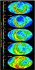 |
Fig. 1 All-sky maps (in Mollweide projection) of the ENA fluxes for five energy channels. The map center is identical to that of the ribbon ring, the ecliptic is indicated with the black line. To help guiding the eye, two auxiliary circles bracket the ribbon. Taken from McComas et al. (2012b), reproduced by permission of the AAS. |
Several hypothesis for the cause of this two- to threefold flux enhancement have been put forward. McComas et al. (2009b) and Schwadron et al. (2009) have been first in suggesting that the ribbon might result from a chain of charge-exchange processes at the end of which the de-charging of a ring distribution of pick-up ions in the local interstellar magnetic field is – given inefficient isotropization (Florinski et al. 2010; Gamayunov et al. 2010) – the source of the ribbon ENAs. While a number of authors followed this idea or variants of it (Chalov et al. 2010; Frisch et al. 2010a,b; Grygorczuk et al. 2011; Heerikhuisen et al. 2010; Heerikhuisen & Pogorelov 2011; Strumik et al. 2011; Möbius et al. 2013), Schwadron & McComas (2013) suggested that the ribbon could be a consequence of a temporary, plasma-wave-induced containment of newly ionized atoms in a spatial “retention” region in the local interstellar medium (ISM). These ions are assumed to be created mainly from neutralized solar wind as well as neutralized pick-up ions from the upstream side of the solar wind termination shock. Fahr et al. (2011) and Siewert et al. (2013) speculated that the direct ion sources of the ribbon ENAs are rather located inside the heliosphere, namely in form of pick-up ions related to adiabatically cooled anomalous cosmic rays upstream of the solar wind termination shock and shock-accelerated pick-up ions beyond. Alternatively, Grzedzielski et al. (2010) proposed the idea that these ENAs could be produced by charge exchange between the neutral hydrogen atoms at the nearby edge of the local interstellar cloud (LIC) and the hot protons of the Local Bubble (LB).
These hypotheses have been summarized and critically assessed by McComas et al. (2011), Schwadron et al. (2011), as well as Schwadron & McComas (2013), with the result that, so far, none of the proposed explanations is without problems, none is generally accepted and, thus, that one cannot exclude the possibility of other scenarios not yet discovered (see, e.g., Pogorelov et al. 2011). In the present paper we present such a new scenario that is consistent with the characteristics of the ribbon, in particular with its likely connection to the orientation of the interstellar magnetic field (Frisch et al. 2010a, 2012). However, rather than involving secondary suprathermal ions in the inner or outer heliosheath or from even farther away, this alternative scenario is related to the inhomogeneous structure of the local ISM itself.
2. Inhomogeneities in the interstellar medium
During recent years tremendous progress has been made regarding the observation and modelling of the large-scale ISM (see, e.g., the reviews by Breitschwerdt et al. 2009; Haffner et al. 2009; Gent 2012), and regarding small-scale (10–100 AU) ionized and neutral structures in the diffuse ISM (Haverkorn & Goss 2007). According to the presently prevailing picture also the neutral hydrogen gas must be considered as a turbulent medium (e.g., Heiles & Troland 2005) and recent corresponding simulation results (Hennebelle & Audit 2007) revealed a rather complex structure: as shown in Figs. 1 to 3 in the latter paper, the number density of the neutral ISM as resulting from a 2D hydrodynamic simulation evolves into a statistical equilibrium. This equilibrium can be characterized by two distinct phases, namely the cold and warm neutral media. These results reveal that particularly also in the warm neutral medium the number density can vary easily by a factor of two and more down to the 400 AU scale and can be expected to vary on still smaller scales, too, as observations suggest (Welty 2007).
Transferring these findings from the general to the local ISM, whose neutral component has the properties of the warm neutral medium (e.g., Stanimirović 2009), it appears rather unlikely that it is homogeneous on scales above a few AU.
Similarly, there are many fluctuations in the plasma down to the AU scale and below (Armstrong et al. 1995; Haverkorn & Spangler 2013) as is manifest in the so-called “big power law in the sky” (Spangler 2007). These fluctuations can not only be coupled to the neutral gas (Shaikh & Zank 2010) but might actually help to form so-called “tiny-scale atomic structures” (Heiles 1997; Cho & Lazarian 2003), i.e. structures in the neutral ISM that could be responsible for the ribbon phenomenon.
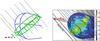 |
Fig. 2 Illustration of the ribbon formation as a result of a neutral density enhancement. Left panel: the blue lines indicated the heliopause, the black lines give the orientation of the undisturbed interstellar magnetic field (ISM) along which a neutral density enhancement (H-wave, see text) with a characteristic scale of a few tens of AU is propagating. Since the actual extent of such disturbance, which is schematically illustrated here by the green cylindrical area, in directions perpendicular to the magnetic field is not important in the present context, the cylinder indicates that part of the disturbance that is of interest for the ribbon formation. Right panel (reproduced by permission of the AAAS): the flux of energetic neutral atoms projected onto the heliopause around which the interstellar magnetic field lines are draping (adopted from McComas et al. 2009b). |
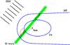 |
Fig. 3 Sketch of the ribbon formation in a plane perpendicular to the orientation of the undisturbed interstellar magnetic field (IMF, black lines). An enhancement of interstellar density (an H-wave, green area) is propagating through the heliosphere that is depicted by the terminaton shock (TS) and the heliopause (HP). In the intersection region, which is indicated by the shaded areas and forms a ring-like structure in 3D, the production rate of ENAs is increased. If in the more distant intersection regions more ENAs of higher energy are produced because of the continued acceleration of protons along the trajectories in the inner heliosheath (two examples are given as the curved red arrows), the ribbon appears under a wider angle in higher energies (as indicated by the three thin dashed solar line-of-sights, for details see text). |
3. The ribbon resulting from a local enhancement in the neutral density
The interpretation of the ribbon as a signature of a local enhancement in the interstellar neutral density requires the existence of corresponding disturbances that are related to the magnetic field orientation. Consequently, such disturbances are unlikely to be the “randomly” distributed clouds like those discussed by, e.g. Frisch et al. (2010b, 2011), but should rather be expected to be of wave- or pulse-like nature. That such disturbances probably exist in a partially ionized plasma is discussed in the following.
First, studies of the propagation of Alfvén, fast magnetosonic, and slow magnetosonic waves in partially ionized, magnetized, astrophysical plasmas have revealed that the first two are strongly damped, but the slow waves, i.e. compressive waves propagating along the magnetic field, are not. While Balsara (1996) has found this for molecular clouds, Zaqarashvili et al. (2011) have demonstrated the same result for the solar atmosphere. Given that this is, thus, found for systems characterized by very different number densities and temperatures the same behaviour can be assumed for the case of the local ISM (see also Haverkorn & Spangler 2013).
Second, it has been shown that disturbances in the plasma and the neutral components are coupled via momentum (e.g., Balsara 1996; Diver et al. 2006; Zaqarashvili et al. 2011) and/or charge transfer (e.g., Shaikh et al. 2006; Kellum & Shaikh 2011, – in fact, the hydrogen wall exists due to the latter process). In particular, it was found that the plasma and neutral fluctuations can be in phase (Diver et al. 2006) and that perturbations in neutral density can propagate along the magnetic field (Zaqarashvili et al. 2011).
With respect to the local ISM such disturbances could be a result of cascading from larger scales (and corresponding coupling to the neutral component) or could be generated at the nearest border of the local cloud the heliosphere is immersed in. This border could be as close as 10.300 AU (e.g., Redfield & Linsky 2000).
In any case, it is likely that there are indeed neutral density enhancements in the vicinity of the heliosphere that propagate along the interstellar magnetic field. While, in principal, the phase front normal could be tilted w.r.t. the field direction, from studies like that by Lerche (1978) and Zaqarashvili et al. (2011) the corresponding angle can be expected to be small. Such density enhancements, which we refer to in the following as “H-waves”, can therefore be envisaged as wall- or sheet-like regions of increased number density in planes perpendicular to the undisturbed interstellar magnetic field as is schematically illustrated in Fig. 2. While during the approach to the heliopause the plasma disturbance propagates along the ISM, which adapts to the shape of the heliopause surface, the H-wave continues a straight motion and enters the heliosphere.
After the crossing of the heliopause, which coincides with the local decoupling of the H-wave from the interstellar plasma flow, the H-wave will at most weakly couple to the plasma of the inner heliosheath. This is because the thickness of the heliosheath, as compared to typical interstellar length scales, is short and, thus, a coupling via charge exchange processes cannot be efficient. This fact is manifest in the limited so-called filtration of neutral hydrogen, which amounts to about 35% across the whole heliospheric interface (i.e. the region between the bow shock/wave and the termination shock) according to the consensus value obtained from hydrodynamic and kinetic models (Müller et al. 2008) or possibly even less (Fahr 2003; Bzowski et al. 2009). Consequently, the dynamics of the plasma in the inner heliosheath cannot be expected to influence the H-wave that, therefore, continues to propagate mainly undisturbed into the heliosphere.
We discuss the consequences of such H-wave for the ENA ribbon in the following.
3.1. Ribbon fluxes
The differential ENA production rate at location r and time τ is given by (see, e.g., Fahr et al. 2007; Sternal et al. 2008) ![\begin{eqnarray} \Psi_{{\rm ENA},{\rm p}}\left(\vec{r},v_{\rm ENA},\tau\right) &=& \left[n_{\rm p}f_{\rm p}\left(v_{\rm p}\right)n_{\rm H}\sigma_{\rm ex} \left(v_{\rm rel}\right)v_{\rm rel}\right]_{\vec{r},\tau} \end{eqnarray}](/articles/aa/full_html/2014/01/aa22064-13/aa22064-13-eq4.png) (1)where vENA is the resulting ENA speed, np and nH are the local proton and hydrogen number densities, and fp(vp) denotes the proton velocity distribution function in the solar wind rest frame. The ENA velocity is given by vENA = usw + vp with the solar wind and (individual) proton velocity usw and vp, respectively. Considering charge transfer with solar wind (and/or pick-up) protons, described by the corresponding cross section σex depending on the mean relative speed vrel of the interaction partners, this production rate is highest in the inner heliosheath, i.e. between the termination shock and the heliopause, see, e.g., Fig. 2 in Sternal et al. (2008).
(1)where vENA is the resulting ENA speed, np and nH are the local proton and hydrogen number densities, and fp(vp) denotes the proton velocity distribution function in the solar wind rest frame. The ENA velocity is given by vENA = usw + vp with the solar wind and (individual) proton velocity usw and vp, respectively. Considering charge transfer with solar wind (and/or pick-up) protons, described by the corresponding cross section σex depending on the mean relative speed vrel of the interaction partners, this production rate is highest in the inner heliosheath, i.e. between the termination shock and the heliopause, see, e.g., Fig. 2 in Sternal et al. (2008).
Integrating along a line-of-sight from an inner boundary (IB) at the detector to an outer boundary (OB) sufficiently beyond the ENA source region, yields the differential ENA flux 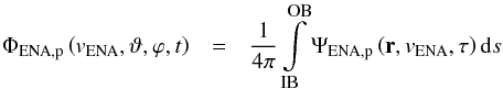 (2)with the heliographic latitude ϑ and longitude ϕ of a given line-of-sight and t = τ + s/vENA, with the distance s between the production and detection location. Corrections for losses were discussed by, e.g., Fahr & Scherer (2004) and Bzowski (2008).
Obviously, this flux is directly proportional to the local neutral number density nH, which is determined by the interstellar neutral density. If the latter is locally increased as the consequence of a traveling slow mode-induced H-wave, also the production of ENAs in the intersection region of the disturbance with the inner heliosheath (see Fig. 3) is increased. This results in a corresponding flux enhancement from a ring-like region – which appears as the ribbon in the all-sky flux maps as shown in Fig. 1.
3.2. Ribbon width
The angular extent of the ribbon is widening with increasing energy (Schwadron et al. 2011; McComas et al. 2012b; Schwadron & McComas 2013), see also Fig. 1 above. This fact can also be understood in the H-wave scenario. Due to the turbulence in the inner heliosheath, solar wind and pick-up protons are expected to be accelerated (e.g., Kallenbach et al. 2005; Florinski 2009). Consequently, the energy distributions should exhibit an increasing fraction of accelerated protons with increasing distance along the flowlines (two examples of which are illustrated in Fig. 3) in the heliosheath. This implies that the lower energy ENAs are produced more towards the termination shock and a comparatively larger part of the intersection region between the H-wave and the heliosheath (shaded areas in Fig. 3) contributes to the ENA flux at higher energies. Obviously, this leads to a ribbon width that is increasing with increasing ENA energy as is indicated with the thin solid and dashed solar line-of-sights.
3.3. Ribbon spectra
In-depth analyses if IBEX data (Dayeh et al. 2011; Livadiotis et al. 2011; Schwadron et al. 2011) have revealed that, despite originally different claims (McComas et al. 2009b), the ribbon ENAs exhibit – following the terminology introduced in Dayeh et al. (2011) – a spectrum with a “knee-shaped” break (i.e. a softening towards higher energies), while those from other regions are characterized by spectra with “ankle-shaped” breaks (i.e. a hardening towards higher energies). Plots comparing the different spectra reveal that the ribbon fluxes are always the highest in the energy range from 1 to 4 keV, see Fig. 3 in Dayeh et al. (2011). Such increased ribbon fluxes can also be understood in terms of the scenario outlined above. On the one hand, all explanations based on a heliospheric source of ENAs (e.g., Fahr et al. 2012; Siewert et al. 2013) would apply as well – an H-wave would simply enhance the effects. On the other hand, one should note that the region where the H-wave intersects the heliopause is possibly also a region of both perturbed plasma (in phase with the neutral perturbation, see Diver et al. 2006) and the strongest deformation of the interstellar magnetic field due to the “obstacle” heliosphere (Schwadron et al. 2009; Pogorelov et al. 2011), see Fig. 2. In such an again ring-like region, where the perturbed interstellar and heliospheric plasmas interact, one can expect increased turbulence. The latter leads to a local stochastic acceleration of protons which, after charge exchange with interstellar hydrogen atoms, results in partially increased differential fluxes of ENAs.
3.4. Ribbon motion
In the proposed scenario the ribbon feature in the ENA flux maps is the result of an H-wave, i.e. a density enhancement related to the slow (magnetosonic) wave in the plasma component (see above). The propagation speed of such wave can be estimated. The fast (+) and slow (−) magnetosonic modes have the phase speeds (e.g., Boyd & Sanderson 2003) ![\begin{eqnarray} V_\pm\! =\! \left\{\frac{1}{2}\left[V_{\rm A}^{2} + V_{\rm S}^{2} \pm \sqrt{(V_{\rm A}^{2} + V_{\rm S}^{2})^2 - 4\, V_{\rm A}^{2}\,V_{\rm S}^{2}\,\cos^2\vartheta} \right]\right\}^{\! 1/2} \!\!\! \end{eqnarray}](/articles/aa/full_html/2014/01/aa22064-13/aa22064-13-eq21.png) (3)where VA and VS are the Alfvén and sound speed, respectively, and ϑ denotes the angle between the wave vector and the magnetic field. For propagation along the magnetic field (ϑ = 0,π) the speed of the slow wave reduces to V− = VS.
(3)where VA and VS are the Alfvén and sound speed, respectively, and ϑ denotes the angle between the wave vector and the magnetic field. For propagation along the magnetic field (ϑ = 0,π) the speed of the slow wave reduces to V− = VS.
The commonly used value for the sound speed in the ISM is VS ≈ 10 km s-1 (e.g., Slavin & Frisch 2002; Redfield & Linsky 2008). Projecting the velocity vector of the Sun relative to the local ISM (McComas et al. 2012a) onto the direction of the velocity vector of the H-wave (aligned with the undisturbed local interstellar magnetic field) yields a speed of the H-wave relative to the Sun of Vrel,H − wave ≈ (23.2cos(α1)cos(α2) ± 10) km s-1 ≈ (17.1 ± 10) km s-1, where α1 = 31.5° and α2 = 30.2° are the longitudinal and latitudinal angular differences between the directions to the heliospheric nose and the ribbon ring center. This translates into a H-wave speed of 1.5 to 5.5 AU/year relative to the Sun. Consequently, with the H-wave scenario one expects a change in the ribbon location. Given the still relatively limited period of available IBEX data, however, the effect can hardly be noticeable so far. This should change on the order of ten years.
3.5. Ribbon fine structure
The fine structure of the ribbon, i.e. its inhomogeneous as well as time-dependent intensity (McComas et al. 2009b, 2012b) can naturally be understood in the suggested scenario of an H-wave: A real, non-idealized wave will, of course, not be a strictly homogeneous “wall” of increased density but exhibit some variations across its main plane. Such internal inhomogeneity can indeed be expected in view of interstellar turbulence as has been studied in preliminary manner by Kota et al. (2011) already.
4. Consequences for the neutral atom fluxes at lower energies
While the discussion, so far, focused on ENAs, one must realize that a wall- or sheet-like neutral density enhancement as described above has implications also for the neutral atoms at lower energies. Low-energy neutral atoms are also observed with IBEX (e.g. Möbius et al. 2009) and a detection of an H-wave from corresponding measurements might, in principle, be possible, as is indicated by the recent identification of discrepancies between (traditional) model expectations and actual IBEX observations (Schwadron et al. 2013). Since is, however, advantageous to inspect other, independent observations that allow for an improved localisation of an H-wave, we discuss Lyman-α measurements made with the Voyager spacecraft in the following.
4.1. Lyman-α intensity in the heliosphere
Particularly, with a glance at the sketch displayed in Fig. 3, the neutral density inside the termination shock will be increased as well. Such observation would be strongly supportive of the outlined idea.
Since the suspected density enhancement is expected to be (presently) localized in the outer heliosphere (see the green area enclosed by the termination shock in Fig. 3) and, thus, cannot be detected with actually operating Lyman-α instruments at 1 AU, one has to inspect the corresponding Voyager data.
These data are presented in Fig. 7 in Quémerais et al. (2009) giving the variation in Lyman-α upwind intensity (normalized to its value at 55 AU and corrected for solar cycle-induced flux variations) measured by the Voyager 1 spacecraft as a function of heliocentric distance. The authors demonstrate that the available models, i.e. a multiple scattering model for a constant density in the outer heliosphere and one using the hydrogen distribution derived from a heliospheric interface model, fail to represent the almost constant value obtained from the data after 70 AU. Evidently, there is a change in slope of the intensity profile that was unexpected based on the results obtained for distances lower than 70 AU (Quémerais et al. 2003). These authors associate the change in slope with a steep increase in the hydrogen number density and state. In addition, the increase is faster that what can be expected from a constant source outside the heliosphere (Quémerais 2006). Simply increasing the neutral hydrogen density does not solve the problem as Quémerais et al. (2003) have already demonstrated, see their Fig. 9. Despite different densities of hydrogen in the local ISM and despite a correspondingly absent or differently positioned and differently structured hydrogen wall, all models fail to reproduce the intensity increase at 70 AU.
Obviously, an inhomogeneity of the interstellar hydrogen like an H-wave potentially explains the observations: The localized intensity increase could be associated with the penetration of an H-wave. From the measurements one can estimate that the leading edge of the H-wave was located at about 70 AU in 1998. It would have been nice to see whether this feature is consistent with Voyager 2 measurements, but that instrument was shut down due to power constraints end of 1998 when the spacecraft was at a heliocentric distance of about 55 AU, i.e. in a region that had not yet been reached by the H-wave.
4.2. Lyman-α absorption outside the heliosphere
It has recently been claimed that IBEX results are not compatible with the existence of a bow shock in the local ISM (McComas et al. 2012a). While this is still under debate (see, e.g., Ben-Jaffel & Ratkiewicz 2012), if true, it has implications for models of the interstellar Lyman-α absorption. Those models, which can be used to obtain information about astrospheres and winds of other stars (for a review see Wood 2004), are usually computed with a so-called two-shock model, i.e. one exhibiting both a termination and a bow shock (e.g., Wood et al. 2007). Removing the bow shock, by effectively assuming a subsonic interstellar flow, still allows to fit the Lyman-α absorption – despite a substantially different hydrogen wall – if the Mach number is taken to be 0.9 (Gayley et al. 1997) or, taking reasonable interstellar magnetic field values into account, if the Alfvénic and fast magnetosonic Mach numbers are 1.09 and 1.03, respectively (Zank et al. 2013), i.e. somewhat higher values than those corresponding to the findings by McComas et al. (2012a). For lower Mach numbers there would be less absorption (Gayley et al. 1997) and the line profiles could not be explained.
This problem would be absent if additional absorbing hydrogen would be in the line-of-sight, just as an inhomogeneous ISM with an H-wave would provide.
5. Conclusions
We have argued that the local ISM is likely not to be as homogeneous as is commonly assumed in, so far, every model of the heliosphere. The charge exchange coupling of the neutral to the plasma component allows for compressive (slow mode) waves in both, which can propagate along the interstellar magnetic field. As a result, the ISM can contain wall- or sheet-like neutral density enhancements oriented in planes perpendicular to the magnetic field.
When propagating through the heliosphere, such an H-wave can not only trigger the higher flux of energetic neutral atoms appearing as the so-called ribbon in all-sky flux maps and explain their energy spectra, but would also account for those absorption features in the Lyman-α lines measured towards nearby stars, which otherwise could not be consistently explained. Observational evidence corroborating the existence of such inhomogeneity comes from heliospheric Lyman-α measurements, which demonstrate that the neutral hydrogen density increased beyond 70 AU.
The present IBEX observations of the ribbon and those to be made in the future potentially with the Interstellar Mapping Probe (IMAP, see National Academy of Sciences 2012) may thus provide a unique opportunity to learn more about the nature of the ISM surrounding the heliosphere.
Acknowledgments
We appreciate discussions with H. J. Fahr, P. C. Frisch, S. Spangler, and G. P. Zank on this topic during the IBEX workshop in Bad Honnef, Germany. The work benefitted from the activities within the research projects FI 706/15-1 and Sche 334/9-1 both funded by the Deutsche Forschungsgemeinschaft (DFG). Work in the US was carried out through the IBEX mission, which is part of NASA’s Explorer Program.
References
- Armstrong, J. W., Rickett, B. J., & Spangler, S. R. 1995, ApJ, 443, 209 [NASA ADS] [CrossRef] [Google Scholar]
- Balsara, D. S. 1996, ApJ, 465, 775 [NASA ADS] [CrossRef] [Google Scholar]
- Ben-Jaffel, L., & Ratkiewicz, R. 2012, A&A, 546, A78 [NASA ADS] [CrossRef] [EDP Sciences] [Google Scholar]
- Boyd, T. J. M., & Sanderson, J. J. 2003, The Physics of Plasmas (Cambridge University Press) [Google Scholar]
- Breitschwerdt, D., de Avillez, M. A., Fuchs, B., & Dettbarn, C. 2009, Space Sci. Rev., 143, 263 [NASA ADS] [CrossRef] [Google Scholar]
- Bzowski, M. 2008, A&A, 488, 1057 [NASA ADS] [CrossRef] [EDP Sciences] [Google Scholar]
- Bzowski, M., Möbius, E., Tarnopolski, S., Izmodenov, V., & Gloeckler, G. 2009, Space Sci. Rev., 143, 177 [NASA ADS] [CrossRef] [Google Scholar]
- Chalov, S. V., Alexashov, D. B., McComas, D., et al. 2010, ApJ, 716, L99 [NASA ADS] [CrossRef] [Google Scholar]
- Cho, J., & Lazarian, A. 2003, MNRAS, 345, 325 [NASA ADS] [CrossRef] [Google Scholar]
- Dayeh, M. A., McComas, D. J., Livadiotis, G., et al. 2011, ApJ, 734, 29 [NASA ADS] [CrossRef] [Google Scholar]
- Diver, D. A., Potts, H. E., & Teodoro, L. F. A. 2006, New J. Phys., 8, 265 [NASA ADS] [CrossRef] [Google Scholar]
- Fahr, H. J. 2003, Ann. Geophys., 21, 1289 [NASA ADS] [CrossRef] [Google Scholar]
- Fahr, H.-J., & Scherer, K. 2004, Astrophys. Space Sci. Trans., 1, 3 [Google Scholar]
- Fahr, H., Fichtner, H., & Scherer, K. 2007, Rev. Geophys., 45, RG4003 [Google Scholar]
- Fahr, H.-J., Siewert, M., McComas, D. J., & Schwadron, N. A. 2011, A&A, 531, A77 [NASA ADS] [CrossRef] [EDP Sciences] [Google Scholar]
- Fahr, H. J., Chashei, I. V., & Siewert, M. 2012, A&A, 537, A95 [NASA ADS] [CrossRef] [EDP Sciences] [Google Scholar]
- Florinski, V. 2009, Space Sci. Rev., 143, 111 [NASA ADS] [CrossRef] [Google Scholar]
- Florinski, V., Zank, G. P., Heerikhuisen, J., Hu, Q., & Khazanov, I. 2010, ApJ, 719, 1097 [NASA ADS] [CrossRef] [Google Scholar]
- Frisch, P. C., Andersson, B.-G., Berdyugin, A., et al. 2010a, ApJ, 724, 1473 [NASA ADS] [CrossRef] [Google Scholar]
- Frisch, P. C., Heerikhuisen, J., Pogorelov, N. V., et al. 2010b, ApJ, 719, 1984 [NASA ADS] [CrossRef] [Google Scholar]
- Frisch, P. C., Redfield, S., & Slavin, J. D. 2011, ARA&A, 49, 237 [NASA ADS] [CrossRef] [Google Scholar]
- Frisch, P. C., Andersson, B.-G., Berdyugin, A., et al. 2012, ApJ, 760, 106 [NASA ADS] [CrossRef] [Google Scholar]
- Fuselier, S. A., Allegrini, F., Funsten, H. O., et al. 2009, Science, 326, 962 [NASA ADS] [CrossRef] [Google Scholar]
- Gamayunov, K., Zhang, M., & Rassoul, H. 2010, ApJ, 725, 2251 [NASA ADS] [CrossRef] [Google Scholar]
- Gayley, K. G., Zank, G. P., Pauls, H. L., Frisch, P. C., & Welty, D. E. 1997, ApJ, 487, 259 [NASA ADS] [CrossRef] [Google Scholar]
- Gent, F. A. 2012, Space Sci. Rev., 166, 281 [NASA ADS] [CrossRef] [Google Scholar]
- Grygorczuk, J., Ratkiewicz, R., Strumik, M., & Grzedzielski, S. 2011, ApJ, 727, L48 [NASA ADS] [CrossRef] [Google Scholar]
- Grzedzielski, S., Bzowski, M., Czechowski, A., et al. 2010, ApJ, 715, L84 [NASA ADS] [CrossRef] [Google Scholar]
- Haffner, L. M., Dettmar, R.-J., Beckman, J. E., et al. 2009, Rev. Mod. Phys., 81, 969 [NASA ADS] [CrossRef] [Google Scholar]
- Haverkorn, M., & Goss, W. M. 2007, SINS – Small Ionized and Neutral Structures in the Diffuse Interstellar Medium, ASP Conf. Ser., 365 [Google Scholar]
- Haverkorn, M., & Spangler, S. R. 2013, Space Sci. Rev., 178, 483 [NASA ADS] [CrossRef] [Google Scholar]
- Heerikhuisen, J., & Pogorelov, N. V. 2011, ApJ, 738, 29 [NASA ADS] [CrossRef] [Google Scholar]
- Heerikhuisen, J., Pogorelov, N. V., Zank, G. P., et al. 2010, ApJ, 708, L126 [NASA ADS] [CrossRef] [Google Scholar]
- Heiles, C. 1997, ApJ, 481, 193 [NASA ADS] [CrossRef] [Google Scholar]
- Heiles, C., & Troland, T. H. 2005, ApJ, 624, 773 [NASA ADS] [CrossRef] [Google Scholar]
- Hennebelle, P., & Audit, E. 2007, in SINS – Small Ionized and Neutral Structures in the Diffuse Interstellar Medium, eds. M. Haverkorn, & W. M. Goss, ASP Conf. Ser., 365, 133 [Google Scholar]
- Kallenbach, R., Hilchenbach, M., Chalov, S. V., Le Roux, J. A., & Bamert, K. 2005, A&A, 439, 1 [NASA ADS] [CrossRef] [EDP Sciences] [Google Scholar]
- Kellum, M. E., & Shaikh, D. 2011, J. Plasma Phys., 77, 577 [NASA ADS] [CrossRef] [Google Scholar]
- Kota, J., Jokipii, J. R., Hsieh, K., & Giacalone, J. 2011, AGU Fall Meeting Abstracts, B1963 [Google Scholar]
- Lerche, I. 1978, Ap&SS, 57, 233 [NASA ADS] [CrossRef] [Google Scholar]
- Livadiotis, G., McComas, D. J., Dayeh, M. A., Funsten, H. O., & Schwadron, N. A. 2011, ApJ, 734, 1 [NASA ADS] [CrossRef] [Google Scholar]
- McComas, D. J., Allegrini, F., Bochsler, P., et al. 2009a, Space Sci. Rev., 146, 11 [NASA ADS] [CrossRef] [Google Scholar]
- McComas, D. J., Allegrini, F., Bochsler, P., et al. 2009b, Science, 326, 959 [NASA ADS] [CrossRef] [PubMed] [Google Scholar]
- McComas, D. J., Funsten, H. O., Fuselier, S. A., et al. 2011, Geophys. Res. Lett., 38, 18101 [NASA ADS] [CrossRef] [Google Scholar]
- McComas, D. J., Alexashov, D., Bzowski, M., et al. 2012a, Science, 336, 1291 [NASA ADS] [CrossRef] [Google Scholar]
- McComas, D. J., Dayeh, M. A., Allegrini, F., et al. 2012b, ApJS, 203, 1 [NASA ADS] [CrossRef] [Google Scholar]
- Möbius, E., Bochsler, P., Bzowski, M., et al. 2009, Science, 326, 969 [NASA ADS] [CrossRef] [Google Scholar]
- Möbius, E., Liu, K., Funsten, H., Gary, S. P., & Winske, D. 2013, ApJ, 766, 129 [NASA ADS] [CrossRef] [Google Scholar]
- Müller, H.-R., Florinski, V., Heerikhuisen, J., et al. 2008, A&A, 491, 43 [NASA ADS] [CrossRef] [EDP Sciences] [Google Scholar]
- National Academy of Sciences 2012, in Solar and Space Physics: A Science for a Technological Society [Google Scholar]
- Pogorelov, N. V., Heerikhuisen, J., Zank, G. P., et al. 2011, ApJ, 742, 104 [NASA ADS] [CrossRef] [Google Scholar]
- Quémerais, E. 2006, in The Physics of the Heliospheric Boundaries, eds. V. V. Izmodenov, & R. Kallenbach, 283 [Google Scholar]
- Quémerais, E., Bertaux, J.-L., Lallement, R., Sandel, B. R., & Izmodenov, V. 2003, J. Geophys. Res., 108, 8029 [CrossRef] [Google Scholar]
- Quémerais, E., Lallement, R., Sandel, B. R., & Clarke, J. T. 2009, Space Sci. Rev., 143, 151 [NASA ADS] [CrossRef] [Google Scholar]
- Redfield, S., & Linsky, J. L. 2000, ApJ, 534, 825 [NASA ADS] [CrossRef] [Google Scholar]
- Redfield, S., & Linsky, J. L. 2008, ApJ, 673, 283 [NASA ADS] [CrossRef] [Google Scholar]
- Schwadron, N. A., & McComas, D. J. 2013, ApJ, 764, 92 [NASA ADS] [CrossRef] [Google Scholar]
- Schwadron, N. A., Bzowski, M., Crew, G. B., et al. 2009, Science, 326, 966 [NASA ADS] [CrossRef] [PubMed] [Google Scholar]
- Schwadron, N. A., Allegrini, F., Bzowski, M., et al. 2011, ApJ, 731, 56 [NASA ADS] [CrossRef] [Google Scholar]
- Schwadron, N., Möbius, E., Kucharek, H., et al. 2013, ApJ, in press [Google Scholar]
- Shaikh, D., & Zank, G. P. 2010, Phys. Lett. A, 374, 4538 [NASA ADS] [CrossRef] [Google Scholar]
- Shaikh, D., Zank, G. P., & Pogorelov, N. 2006, in Physics of the Inner Heliosheath, eds. J. Heerikhuisen, V. Florinski, G. P. Zank, & N. V. Pogorelov, AIP Conf. Ser., 858, 314 [Google Scholar]
- Siewert, M., Fahr, H.-J., McComas, D. J., & Schwadron, N. A. 2013, A&A, 551, A58 [NASA ADS] [CrossRef] [EDP Sciences] [Google Scholar]
- Slavin, J. D., & Frisch, P. C. 2002, ApJ, 565, 364 [NASA ADS] [CrossRef] [Google Scholar]
- Spangler, S. 2007, BAAS, 39, 162 [NASA ADS] [Google Scholar]
- Stanimirović, S. 2009, Space Sci. Rev., 143, 291 [NASA ADS] [CrossRef] [Google Scholar]
- Sternal, O., Fichtner, H., & Scherer, K. 2008, A&A, 477, 365 [NASA ADS] [CrossRef] [EDP Sciences] [Google Scholar]
- Strumik, M., Ben-Jaffel, L., Ratkiewicz, R., & Grygorczuk, J. 2011, ApJ, 741, L6 [NASA ADS] [CrossRef] [Google Scholar]
- Welty, D. E. 2007, in SINS – Small Ionized and Neutral Structures in the Diffuse Interstellar Medium, eds. M. Haverkorn, & W. M. Goss, ASP Conf. Ser., 365, 86 [Google Scholar]
- Wood, B. E. 2004, Liv. Rev. Sol. Phys., 1, 2 [Google Scholar]
- Wood, B. E., Izmodenov, V. V., Linsky, J. L., & Malama, Y. G. 2007, ApJ, 657, 609 [NASA ADS] [CrossRef] [Google Scholar]
- Zank, G. P., Heerikhuisen, J., Wood, B. E., et al. 2013, ApJ, 763, 20 [NASA ADS] [CrossRef] [Google Scholar]
- Zaqarashvili, T. V., Khodachenko, M. L., & Rucker, H. O. 2011, A&A, 529, A82 [NASA ADS] [CrossRef] [EDP Sciences] [Google Scholar]
All Figures
|
Fig. 1 All-sky maps (in Mollweide projection) of the ENA fluxes for five energy channels. The map center is identical to that of the ribbon ring, the ecliptic is indicated with the black line. To help guiding the eye, two auxiliary circles bracket the ribbon. Taken from McComas et al. (2012b), reproduced by permission of the AAS. |
| In the text | |
|
Fig. 2 Illustration of the ribbon formation as a result of a neutral density enhancement. Left panel: the blue lines indicated the heliopause, the black lines give the orientation of the undisturbed interstellar magnetic field (ISM) along which a neutral density enhancement (H-wave, see text) with a characteristic scale of a few tens of AU is propagating. Since the actual extent of such disturbance, which is schematically illustrated here by the green cylindrical area, in directions perpendicular to the magnetic field is not important in the present context, the cylinder indicates that part of the disturbance that is of interest for the ribbon formation. Right panel (reproduced by permission of the AAAS): the flux of energetic neutral atoms projected onto the heliopause around which the interstellar magnetic field lines are draping (adopted from McComas et al. 2009b). |
| In the text | |
|
Fig. 3 Sketch of the ribbon formation in a plane perpendicular to the orientation of the undisturbed interstellar magnetic field (IMF, black lines). An enhancement of interstellar density (an H-wave, green area) is propagating through the heliosphere that is depicted by the terminaton shock (TS) and the heliopause (HP). In the intersection region, which is indicated by the shaded areas and forms a ring-like structure in 3D, the production rate of ENAs is increased. If in the more distant intersection regions more ENAs of higher energy are produced because of the continued acceleration of protons along the trajectories in the inner heliosheath (two examples are given as the curved red arrows), the ribbon appears under a wider angle in higher energies (as indicated by the three thin dashed solar line-of-sights, for details see text). |
| In the text | |
Current usage metrics show cumulative count of Article Views (full-text article views including HTML views, PDF and ePub downloads, according to the available data) and Abstracts Views on Vision4Press platform.
Data correspond to usage on the plateform after 2015. The current usage metrics is available 48-96 hours after online publication and is updated daily on week days.
Initial download of the metrics may take a while.