© ESO, 2014

1. Introduction

The BLS algorithm for identifying transiting exoplanets (Kovács et al. 2002, hereafter KZM) is very widely used. While this work uses BLS as a concrete example, we stress that the main questions we address here are related to the information content of the data, and are therefore easily translatable to other detection algorithms. Compared to other period-searching algorithms, such as Fourier transform or Lomb-Scargle periodograms, the computational load of BLS is rather high. This is an opposite conclusion to that of KZM since – as we show here – looking for transits requires many more frequency steps than looking for sine-like variations. Recently this situation has became particularly grave since both space – and ground – based surveys now span several years and have obtained hundreds of thousands of light curves (if not millions) so that their BLS analysis quickly becomes a challenge. In this paper we show that optimally scanning the BLS parameters, even without changing the BLS core technique, can produce very significant performance improvements and improve sensitivity over standard practices at the same time.

The BLS technique fits a box of some phase duration to a light curve folded at some test frequency, at all possible starting times – producing a three-dimensional search in orbital frequency, reference phase and duty cycle. For this reason the current work is also similarly divided: after defining the duty cycle in Sect. 2, we discuss the frequency search axis in Sect. 3, and the reference phase and duty cycle search axes in Sect. 4. Finally, we discuss whether and how to choose the best-fitting frequency in Sect. 5 and conclude in Sect. 6.

2. The transit signal duty cycle

BLS aims at detecting a periodic sudden and short drop in the observed flux, ostensibly caused by a transiting planet. The orbital period of a test particle around the host star, such as a planet, is given in Keplerian dynamics by $\begin{array}{ccc}{\mathit{P}}^{\mathrm{2}}\mathrm{=}\frac{\mathrm{4}{\mathit{\pi }}^{\mathrm{2}}}{\mathit{GM}}{\mathit{a}}^{\mathrm{3}}\mathrm{·}& & \end{array}$(1)Consequently, the phase duration, also known as the duty cycle, of a central transit in a large (a ≫ R) circular orbit with a period P (1/orbital frequency f) around a star with mass and radius M and R, respectively, is $\begin{array}{ccc}\mathit{q}\mathrm{\left(}\mathit{f,M,R}\mathrm{\right)}\mathrm{\approx }\frac{\mathit{R}}{\mathit{\pi a}}\mathrm{=}\frac{\mathrm{(}\mathrm{2}\mathit{\pi }{\mathrm{)}}^{\mathrm{2}\mathit{/}\mathrm{3}}}{\mathit{\pi }}\frac{\mathit{R}}{\mathrm{(}\mathit{GM}{\mathrm{)}}^{\mathrm{1}\mathit{/}\mathrm{3}}}{\mathit{f}}^{\mathrm{2}\mathit{/}\mathrm{3}}& & \end{array}$(2)where a is the orbital semimajor axis.

The observed duty cycle may be shorter than q(f,M,R), for example in non-central transits, or even longer than q(f,M,R), if R is underestimated or M is overestimated. Eccentric orbits may further change the observed duty cycle to both shorter and longer than q(f,M,R), but eccentricity cannot (usually) be detected or even constrained from photometry alone, so for the remainder of this work we assume circular orbits. Still, the quoted q(f,M,R) is our a priori expected duty cycle, and any corrections for longer or shorter duty cycles – as discussed in Sect. 4 – should be made relative to this number.

Important is that the typical targets for transit surveys are solar-type stars which are all approximately similar in mass and size (a factor of 2 in either is very significant), while the orbital period can easily change over three orders of magnitudes – from less than a day to a year and longer. Therefore, for optimizing the transit search, the accuracy of the estimated M and R are far less important, and for the remainder of this work we assume solar values for these parameters when giving numerical results. We note that while the original BLS did not require input of M and R at all, assumptions about the stellar mass and radius were always made, even if implicitly, by the definition of the other search parameters. By making them explicit we allow correcting for non-solar values, such as in proposed searches for transiting planets around white dwarfs (Agol 2011).

3. The frequency axis

3.1. Search edges

The available dataset will be described by a single parameter: its span in time, hereafter simply span and labeled S. The minimal search frequency is naturally derived from the goal of detecting periodic phenomena, so the maximum period can be no longer than half of the data span, or ${\mathit{f}}_{\min }\mathrm{=}\frac{\mathrm{2}}{\mathit{S}}$. One may prefer to use a more conservative ${\mathit{f}}_{\min }\mathrm{=}\frac{\mathrm{3}}{\mathit{S}}$ that will help to separate similar but unrelated events from true periodicity by requiring observation of a third event – but we will use the former definition below.

The maximal possible frequency could in principle be derived from the Shannon-Nyquist sampling theorem had we known the sampling frequency of our data, but a much more stringent limit usually comes from astrophysical arguments. By setting the orbital distance a in Eq. (1) to 3R (scale of the Roche limit) one can determine the maximal frequency to search: 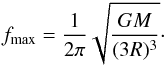$\begin{array}{ccc}{\mathit{f}}_{\max }\mathrm{=}\frac{\mathrm{1}}{\mathrm{2}\mathit{\pi }}\sqrt{\frac{\mathit{GM}}{\mathrm{(}\mathrm{3}\mathit{R}{\mathrm{)}}^{\mathrm{3}}}}\mathrm{·}& & \end{array}$(3)Searching the range [ f_min,f_max ] will ensure that all relevant orbital periods are covered (down to about 14.5 h for the Sun).

3.2. Frequency resolution

When searching for transit signals it is commonly assumed that one should uniformly sample the orbital frequency rather than the orbital period (e.g. KZM). However, while this is true for sine-like signals, including the additional information that the transit duty cycle is also frequency-dependent changes that picture.

The frequency resolution of uniformly-sampled sine signals is $\frac{\mathrm{1}}{\mathit{S}}$. In the context of experimental data this is the width of the Fourier transform peak. We wish to find the corresponding number for transit-like signals. We assume our signal was uniformly sampled and that it has an exact box shape, i.e.: when folded on the true frequency f_true only the points in a small phase range spanning q_true(f_true,M,R) are all at some definite non-zero value, and all other points have a value of zero. We now consider an imperfect folding at some frequency f_true + Δf: in such a case each point is shifted (relative to the exact case) by (Δf·t) phase when t is the data point’s time. If the reference time is the beginning of the dataset then on average points move by (Δf·S/2) phase. The probability that such a shift will move the point to outside the true box is approximately the ratio of the phase shift to the box sizes $\frac{\mathrm{\Delta }\mathit{f}\mathrm{·}\mathit{S}\mathit{/}\mathrm{2}}{\mathit{q}\mathrm{(}{\mathit{f}}_{\mathrm{true}}\mathit{,M,}\hspace{0.17em}\mathit{R}\mathrm{)}}$. Since the BLS score (labeled “Signal Residue” by KZM) scales with the number of points in transit, this is also the relative change in the BLS score due to Δf. To find the half width at half maximum (HWHM) of the BLS peak (which is a measure of frequency resolution) we set the condition for the BLS score to half its peak value: $\frac{\mathrm{\Delta }{\mathit{f}}_{\mathrm{HWHM}}\mathrm{·}\mathit{S}\mathit{/}\mathrm{2}}{\mathit{q}\mathrm{\left(}{\mathit{f}}_{\mathrm{true}}\mathit{,M,R}\mathrm{\right)}}\mathrm{=}\frac{\mathrm{1}}{\mathrm{2}}$ or: $\mathrm{\Delta }{\mathit{f}}_{\mathrm{HWHM}}\mathrm{=}\frac{\mathit{q}\mathrm{\left(}{\mathit{f}}_{\mathrm{true}}\mathit{,M,R}\mathrm{\right)}}{\mathit{S}}$. In the presence of an unknown f_true one needs to oversample this critical frequency resolution to be sure that the peak is not just missed between frequency samples. We therefore add a frequency oversampling parameter OS which is the number of frequency points to calculate in the expected HWHM range to give the final $\begin{array}{ccc}\mathrm{\Delta }\mathit{f}\mathrm{=}\frac{\mathit{q}\mathrm{\left(}{\mathit{f}}_{\mathrm{true}}\mathit{,M,R}\mathrm{\right)}}{\mathit{S}\mathrm{·}\mathit{OS}}\mathrm{·}& & \end{array}$(4)OS values of the order of a few (2–5) would suffice ensure the true peak is not missed. It is now easy to see that the frequency resolution Δf is no longer constant – it depends on f itself due to the physics of the problem. Also, one can compare this result to the classical frequency resolution of $\frac{\mathrm{1}}{\mathit{S}}$ to find that in the framework presented here sine functions of all frequencies have a constant effective duty cycle of 1, and indeed sine waves are (almost) always non-zero.

The above result means that if one chooses a uniform frequency sampling with Δf_uniform that is suitable for short-period signals (i.e., large Δf) a large portion of the long-period signals will be missed between frequency samples and will not be detected. Conversely, if one chooses a uniform frequency sampling with Δf_uniform than is suitable for long-period signals (i.e., small Δf), the computation time will be artificially increased by a large factor (see next subsection).

Actually, the latter choice will not just be slow to calculate but also it will be less sensitive to real signals by being too sensitive to noise: such a choice will allow “detection” of signals that are extremely unlikely to be transits. For e.g.: a low duty cycle q = 10^-3 is quite possible for a 1yr planet, but the same q means a <4.5 min long transit for a 3 d period – so by allowing such q values one becomes sensitive to phenomena that are more likely to be noise than signals, and so the BLS background noise increases.

3.3. Optimal frequency sampling

Since it was shown above that a uniform frequency sampling law is not optimal, we wish to find the optimal frequency sampling sequence. This means solving the differential equation (Eq. (4)): $\begin{array}{ccc}\mathrm{d}\hspace{0.17em}\mathit{f}& \mathrm{=}& \mathit{A}{\mathit{f}}^{\mathrm{2}\mathit{/}\mathrm{3}}\\ \mathit{A}& \mathrm{\equiv }& \frac{\mathrm{(}\mathrm{2}\mathit{\pi }{\mathrm{)}}^{\mathrm{2}\mathit{/}\mathrm{3}}}{\mathit{\pi }}\frac{\mathit{R}}{\mathrm{(}\mathit{GM}{\mathrm{)}}^{\mathrm{1}\mathit{/}\mathrm{3}}}\frac{\mathrm{1}}{\mathit{S}\mathrm{·}\mathit{OS}}\mathrm{·}\end{array}$(5)By introducing a temporary variable x = 1,2,3,... which is the index number of the sequence of f values, we solve Eq. (5): $\begin{array}{ccc}\mathit{f}\mathrm{\left(}\mathit{x}\mathrm{\right)}\mathrm{=}{\left(\frac{\mathit{A}}{\mathrm{3}}\mathit{x}\mathrm{+}\mathit{C}\right)}^{\mathrm{3}}& & \\ \mathit{C}\mathrm{\equiv }{\mathit{f}}_{\min }^{\mathrm{1}\mathit{/}\mathrm{3}}\mathrm{-}\frac{\mathit{A}}{\mathrm{3}}\mathrm{·}& & \end{array}$(6)Where C is the constant of integration, and by requiring that the first value in the sequence (x = 1) to be f_min its value is determined. This is a non-trivial result: we have shown that for transit surveys the optimal frequency sampling is cubic in frequency, and not linear.

Now we can count the number of frequency steps in the above optimal sampling: $\begin{array}{ccc}{\mathit{N}}_{\mathrm{freq}\mathit{,}\hspace{0.17em}\mathrm{optimal}}\mathrm{=}\left({\mathit{f}}_{\max }^{\mathrm{1}\mathit{/}\mathrm{3}}\mathrm{-}{\mathit{f}}_{\min }^{\mathrm{1}\mathit{/}\mathrm{3}}\mathrm{+}\frac{\mathit{A}}{\mathrm{3}}\right)\frac{\mathrm{3}}{\mathit{A}}\mathrm{·}& & \end{array}$(7)For comparison, uniform sampling suitable for long periods detection has $\mathrm{\Delta }\mathit{f}\mathrm{=}\frac{\mathit{q}\mathrm{(}{\mathit{f}}_{\min }\mathit{,M,}\hspace{0.17em}\mathit{R}\mathrm{)}}{\mathit{S}\mathrm{·}\mathit{OS}}\mathrm{=}\mathit{A}{\mathit{f}}_{\min }^{\mathrm{2}\mathit{/}\mathrm{3}}$, which translates to number of steps of: $\begin{array}{ccc}{\mathit{N}}_{\mathrm{freq}\mathit{,}\hspace{0.17em}\mathrm{uniform}}\mathrm{=}\frac{{\mathit{f}}_{\max }\mathrm{-}{\mathit{f}}_{\min }}{\mathit{A}{\mathit{f}}_{\min }^{\mathrm{2}\mathit{/}\mathrm{3}}}\mathrm{·}& & \end{array}$(8)For a numerical example, in the case of a 3 yr light curve of a Sun-like star (which is typical of the available Kepler data) this means that using uniform sampling is $\frac{{\mathit{N}}_{\mathrm{freq}\mathit{,}\hspace{0.17em}\mathrm{uniform}}}{{\mathit{N}}_{\mathrm{freq}\mathit{,}\hspace{0.17em}\mathrm{optimal}}}\mathrm{=}\mathrm{39}$ times slower than using optimal frequency sampling (see Fig. 1), while not offering improved sensitivity relative to the optimal sampling (actually, the other way around, see Sect. 3.2).

Fig. 1 Number of frequency steps required by a uniform sampling scheme (upper, blue line) and the optimal sampling scheme (lower, greem line). Vertical dashed lines represent the time span of some existing and expected ground- and space-based datasets.

Finally, we comment that since different frequencies can be evaluated independently the Optimal BLS code we make available also allows for parallel evaluation of BLS in the frequency axis on different threads¹. The contribution of multithreading to Optimal BLS performance obviously depends on the used computer system. However, we observed a less than linear performance gain when scaling the thread count, and we guess it is related to the fact that each one of the many frequencies (> 10⁵ frequencies for a 3 yr data) takes only a very short time to calculate so the communication overhead is significant. We therefore recommend using multithreading only for the the manual evaluation of one/few objects, which is required when more attention is given to specific systems. For large scale processing we recommend using the different threads to process different groups (which requires no communication, and also strengthens the case for not-too-large groups, where the concept of BLS groups is explained in Sect. 4.4).

4. On the folded light curve

KZM showed that computing the BLS metric using the original data points is computationally wasteful since virtually the same result can be obtained using phase-binned data – as long as the bin size is small enough so that at least one bin would fall completely in-transit, and not only partially so. We therefore describe below the binless and binned BLS parameters, where the former describes more accurately the possible true signals and the latter is the corresponding parametrization of Optimal BLS.

4.1. Binless BLS

Duty cycle axis:

in this section we assume that the data was already folded at some test frequency f_test. We therefore expect that a central transit would have a duty cycle of q(f_test,M,R). However, as mentioned above, the observed transit can be both longer or shorter. Importantly, extreme circumstances are required for the observed transit to be more than a few times longer or shorter than the expected q(f_test,M,R). We can therefore parameterize factors 1/Q_min > 1 and Q_max > 1 such that we wish to look at test duty cycles q_test in the range $\begin{array}{ccc}\frac{\mathrm{1}}{{\mathit{Q}}_{\min }}\mathit{<}\frac{{\mathit{q}}_{\mathrm{test}}}{\mathit{q}\mathrm{\left(}{\mathit{f}}_{\mathrm{test}}\mathit{,M,R}\mathrm{\right)}}\mathit{<}{\mathit{Q}}_{\max }& & \end{array}$(9)and expect that both 1/Q_min and Q_max to have a value of a few: probably no more than about 3, and with only extreme cases reaching to 5 or higher values.

The reference phase axis:

the reference phase (the mid-transit phase) can have any value between 0 and 1, and all points should be checked in principle. However, there is little gain in setting the reference phase resolution to much smaller than q(f_test,M,R) itself, since the number of in-transit points will not change significantly.

4.2. BLS with binning

Duty cycle axis:

when one bins the data one loses some sensitivity by not optimally using the data in the bins that contain either the ingress or the egress. This effect can be minimized by using a large number of small bins, but then the computational benefit of binning erodes. We show how to properly choose the bin size to find a good balance between the speed of computation and sensitivity. The binless Q_min and Q_max parameters above are used to define their binned counterparts MinBin and NumBins in the following way: since one needs at least one bin to be completely in-transit the minimum bin size should be smaller than the smallest expect transit q(f_test,M,R)/Q_min by some factor MinBin. Larger expected transits up to Q_max would be fitted using an integer number of this minimum-sized bin given by NumBins. Mathematically this means that $\begin{array}{ccc}\mathrm{smallestbinsize}\mathrm{=}\frac{\mathit{q}\mathrm{\left(}{\mathit{f}}_{\mathrm{test}}\mathit{,M,R}\mathrm{\right)}\mathit{/}{\mathit{Q}}_{\min }}{\mathit{MinBin}}\mathrm{·}& & \end{array}$(10)MinBin should be larger than 2 to be sensitive to transits q(f_test,M,R)/Q_min long regardless of the true transit phase, and should have a value of a few (i.e., not a large number) to reduce the computational load. To avoid confusion, we stress that Q_min and Q_max describe the underlying transit signals that we want to search for, while MinBin and NumBins describe the search grid.

Longer transits will be searched using groups of bins, or a bin width of an integer multiple of this smallest bin size. The longest expected transit would have a duration that is Q_min·Q_max times the shortest expected transit, so the largest number of bins to be searched is $\begin{array}{ccc}\mathit{NumBins}\mathrm{=}{\mathit{Q}}_{\min }\mathrm{·}{\mathit{Q}}_{\max }\mathrm{·}& & \end{array}$(11)

The reference phase axis:

using such a binning scheme would allow signals to be readily detected even if their reference time is shifted with respect to the used bins grid, since there will always be at least one bin which is completely in-transit. One therefore still has to check all possible reference phases, but now at a reduced resolution of the bins, which is automatically not much smaller than q(f_test,M,R).

4.3. The computational load

The configurations that need to be checked are all NumBins possible widths, starting from all (smallest bin size)^-1 possible reference phases. Importantly, when optimally binning, the computational load of the individual test frequencies also depends on q(f_test,M,R), meaning that again the choice of a constant bin size incurs penalties. Specifically, the number of configurations to check by using optimal binning is: $\begin{array}{ccc}{\mathit{N}}_{\mathrm{conf}\mathit{.}\mathit{,}\mathrm{optimal}}\mathrm{\left(}{\mathit{f}}_{\mathrm{test}}\mathrm{\right)}\mathrm{=}\mathit{NumBins}\mathrm{·}\frac{\mathit{MinBin}\mathrm{·}{\mathit{Q}}_{\min }}{\mathit{q}\mathrm{\left(}{\mathit{f}}_{\mathrm{test}}\mathit{,M,R}\mathrm{\right)}}\mathrm{·}& & \end{array}$(12)A uniform binning scheme suitable for lone-periods detection would have to scan a different number of configurations: $\begin{array}{ccc}{\mathit{N}}_{\mathrm{conf}\mathit{.}\mathit{,}\mathrm{uniform}}\mathrm{\left(}{\mathit{f}}_{\mathrm{test}}\mathrm{\right)}\mathrm{=}\mathit{NumBins}\mathrm{·}\frac{\mathit{MinBin}\mathrm{·}{\mathit{Q}}_{\min }}{\mathit{q}\mathrm{\left(}{\mathit{f}}_{\min }\mathit{,M,R}\mathrm{\right)}}\mathrm{·}& & \end{array}$(13)Note that by definition of this scheme as uniform it does not have dependency on f_test. The total computational load is just the integration of the number of configurations that need to be checked over all frequencies: $\begin{array}{ccc}{\mathit{N}}_{\mathrm{conf}\mathit{.}\mathit{,}\mathrm{optimal}}& \mathrm{=}& \frac{\mathit{NumBins}\hspace{0.17em}\mathit{MinBin}\hspace{0.17em}{\mathit{Q}}_{\min }}{{\mathit{A}}^{\mathrm{2}}\hspace{0.17em}\mathit{S}\hspace{0.17em}\mathit{OS}}\mathrm{·}\mathrm{3}\mathrm{(}{\mathit{f}}_{\min }^{\mathrm{-}\mathrm{1}\mathit{/}\mathrm{3}}\mathrm{-}{{\mathit{f}}_{\max }^{\mathrm{-}\mathrm{1}\mathit{/}\mathrm{3}}}^{\mathrm{)}}\\ {\mathit{N}}_{\mathrm{conf}\mathit{.}\mathit{,}\mathrm{uniform}}& \mathrm{=}& \frac{\mathit{NumBins}\hspace{0.17em}\mathit{MinBin}\hspace{0.17em}{\mathit{Q}}_{\min }}{{\mathit{A}}^{\mathrm{2}}\hspace{0.17em}\mathit{S}\hspace{0.17em}\mathit{OS}}\mathrm{·}\frac{{\mathit{f}}_{\max }\mathrm{-}{\mathit{f}}_{\min }}{{\mathit{f}}_{\min }^{\mathrm{4}\mathit{/}\mathrm{3}}}\mathrm{·}\end{array}$The total speedup of using optimal sampling and binning is therefore: $\begin{array}{ccc}\mathrm{speedup}\mathrm{=}\frac{{\mathit{N}}_{\mathrm{conf}\mathit{.}\mathit{,}\mathrm{uniform}}}{{\mathit{N}}_{\mathrm{conf}\mathit{.}\mathit{,}\mathrm{optimal}}}\mathrm{=}\frac{{\mathit{f}}_{\max }\mathrm{-}{\mathit{f}}_{\min }}{\mathrm{3}{\mathit{f}}_{\min }^{\mathrm{4}\mathit{/}\mathrm{3}}\hspace{0.17em}\mathrm{(}{\mathit{f}}_{\min }^{\mathrm{-}\mathrm{1}\mathit{/}\mathrm{3}}\mathrm{-}{{\mathit{f}}_{\max }^{\mathrm{-}\mathrm{1}\mathit{/}\mathrm{3}}}^{\mathrm{)}}}\mathrm{·}& & \end{array}$(16)Which for a 3 yr dataset is a very significant speedup factor of 337. For a 8yr dataset the speedup factor is even higher at >880.

4.4. Phase folding

Apart from discussing the BLS calculation on the folded light curve we note that the phase-folding step itself is computationally intensive. When applied to simulated continuous 3 yr long Kepler-like dataset, our optimized implementation spent ~2/3 of the time phase-folding the data. Since for the vast majority of targets in a transit survey there is near-perfect overlap in time stamps (every image of a given field is common to nearly all its targets), these are mostly redundant calculations. Importantly, these redundant calculation will significantly dilute the benefits of Optimal BLS and cause the actual run-time to be longer than suggested by Eq. (16) since phase-folding of the data is sped up only by the factor given by dividing Eq. (8) by Eq. (7).

We therefore allowed for parallel execution of all the BLS calculation steps on multiple stars – so multiple stars are evaluated at each test frequency – and the phase folding is done once for each such group. From practical standpoint, such a group should typically contain several tens of stars (maybe up to a hundred or so) which virtually nullifies the relative time penalty for phase folding, but without incurring a memory penalty by including too large groups. Avoiding too large groups is advisable also since one may not always find enough stars with similar-enough masses and radii (which affect the frequency sampling and phase binning schemes).

When comparing the actual time it takes to calculate BLS on one group using our original and optimized versions, one would expect that due to the above effects the observed speedup factor will be lower than that predicted by Eq. (16) for “groups” of one light curve. On the other hand, the observed speedup factor will approach Eq. (16) for large-enough groups since for them the relative time spent on phase-folding was reduced. This expectation, as well as the speedup scaling with data span (which is the main result of this work), were observed in actual calculations spanning a factor >30 in data spans and a factor of 100 in group sizes (Fig. 2), validating the above analysis.

Fig. 2 Speedup factor of Optimal BLS relative to the unoptimized BLS vs. the span of the simulated dataset (10, 20, 40, 80, 160 and 320 days). The different lines are the ratio of run times measured for different runs, each one for a different group size (1, 10 and 100 stars per group, in blue circles, green squares and red triangles respectively). The solid black line is the predicted speedup factor from Eq. (16) and is not a fit. See text for further discussion.

5. Choosing the best-fitting frequency

5.1. Normalization

Fig. 3 Panel a) optimal BLS spectrum of Kepler’s KOI 1574 (blue) and its BLSternd (red) after removing planet candidate KOI 1574.01 using all available data through Quarter 13. Panel b) same, after removing BLSternd. Panels c), d) two zoomed-in regions with significant local peaks. Optimal frequency sampling is evident by the fact that each peak is sampled with similar number of samples despite the large difference in width.

Obviously, the best-fitting frequency is the one with the highest significance above the background of other tested frequencies. We now consider how to choose this best-fitting frequency, and determine its significance. The first question appears to be trivial as one may simply answer that it would be the frequency with the corresponding highest numerical value of the above BLS run. A first-order answer to the second question was given already by KZM: they defined the signal detection efficiency (SDE) metric by first subtracting the mean of the BLS values and than normalizing to the scatter of the resultant data. This made the SDE naturally scaled: an SDE value of X means that the this particular period is more significant by Xσ than the bulk of checked orbital frequencies.

However, the BLS spectrum of real targets has two important structures that make these choices sub-optimal: (1) there is a rising trend of the BLS values towards lower frequencies, i.e.: the local average of the periodogram rises; (2) there is a rising scatter towards lower frequencies, i.e.: the local scatter around the local average of periodogram increases towards lower frequencies. These two frequency dependencies are expected: as datasets get longer the tested orbital frequencies get lower and so the expected duty cycle at each of these test frequencies q(f_test,M,R) gets smaller. This means that a progressively smaller number of points are actually required to be in-transit, and so the probability that the mean value of smaller groups of random points will be different from the global mean will increase, driving both the mean value and the scatter of the raw BLS spectrum up. Also, the sensitivity to a small number of anomalies or ill-corrected discontinuities will be significantly increased as test frequencies decrease as there will be less data points “in-transit” to average-out such instances. All the above will result in an accelerating rate of changes in the “background” BLS spectrum towards lower frequencies.

In order to solve these problems we slightly generalize the way SDE is calculated:

• instead of removing the mean value, we remove themedian-filtered periodogram. We note that due to the optimalsampling of the frequency axis, peaks at all frequencies nowinclude a similar number of points, so by choosing a median filterwith window size much larger (≥10 times) than the oversampling parameter OS one ensures the peaks of interest are not filtered or attenuated. We label this curve as BLS_ternd(f);

• after removing BLS_ternd we wish to evaluate the local scatter of the data. For that we simply evaluate abs(diff(BLS)) – the absolute value of the point-to-point difference of the periodogram. We then median-smooth that data similarly to the way it was done above, to obtain the local scatter curve – and we label this as curve as BLS_scatter(f);

• our genaralized SDE is now: $\mathrm{SDE}\mathrm{\left(}\mathit{f}\mathrm{\right)}\mathrm{=}\frac{\mathrm{BLS}\mathrm{\left(}\mathit{f}\mathrm{\right)}\mathrm{-}{\mathrm{BLS}}_{\mathrm{ternd}}\mathrm{\left(}\mathit{f}\mathrm{\right)}}{{\mathrm{BLS}}_{\mathrm{scatter}}\mathrm{\left(}\mathit{f}\mathrm{\right)}}\mathrm{·}$

Now the SDE is normalized to better reflect the true significance of a given peak over its local background, even if one chooses a different technique of estimating the local BLS trend and BLS scatter. Some of these effects can be see in Fig. 3: this is the raw Optimal BLS spectrum of a typical target (Kepler’s KIC 10028792, or KOI 1574) spanning 1141 d, after SARS de-correlation (Ofir et al. 2010) and removal of its known giant planet candidate (KOI 1574.01, Batalha et al. 2012). It is easy to see that:

• there is a sharp rise of BLS towards low frequencies: the BLS trendis near-constant above 10^-2 d^-1, or on more than 99% of the frequency range, and practically all the BLS trend variability is below that threshold;

• the local scatter is also increasing towards lower frequencies – from a value of about 1.2 to a value of 3 and more in this particular case. This is best seen by looking at the local scatter of the BLS trend curve;

• the highest peak (at f = 2.615 × 10^-3 d^-1) is the first harmonic of of the 191d planet candidate reported by Ofir & Dreizler (2013). Notably, the width of the peak is a few times 10^-6 d^-1 (panel c). This width can be compared to another peak (panel d) at P ~ 5.83 d (f ~ 0.171 d^-1) which has a width of ~10^-4 d^-1, or several tens of times wider. With SDE > 32 this additional peak is not noise: it (and the adjacent peak at f ≈ 0.111 too) correspond to two new candidate that were not detected by the Kepler pipeline² and are now reported in (Ofir et al., in prep.), despite their raw BLS score being much lower than the corresponding low-frequency background;

• apart from the general trend, there are several additional rather sharp breaks in the BLS spectrum (especially visible on the trend curve). Due to these jumps the BLS trend curve cannot be well-modeled by a simple function like a polynomial, and a numerical function like a median filter (but not limited to it) may perform better.

The last remaining issue is to determine the threshold value above which candidate signals should be considered as probable real detections.

Fig. 4 The (absolute value) fractional difference between injected and detected period, vs. SDE for 1000 simulated signals in 100 d long light curves. The vertical separation between good detections (lower points cloud) and misses (upper points cloud) increases as the data span increases, and here these are already well separated. Importantly, there is not a single missed signal with SDE > 15.

5.2. Significance threshold

We simulated 1000 light curves, all spanning 100 d and containing transit signals of various periods, durations and depths both above and below the detection threshold. The light curves were rather benign in the sense that they included white noise only, and no jumps or discontinuities were simulated. We then compared the detected and simulated periods, and plotted the absolute value of their fractional difference against the SDE (as defined above) of that detected period (see Fig. 4). The separation between good detection and misses is clear. Importantly, all the misses also had low SDE, so the false alarm rate (a detection when there is no signal) is very low for SDE > 15. We conclude that detections of approximately this significance and higher should be promoted to the next level of checks (which is beyond the scope of this paper).

6. Discussion

The Kepler public archive³ currently includes about 200 000 stars monitored for about three years. The ground-based SuperWASP survey public archive⁴ is much larger, holding almost 1.8 × 10⁷ unique light curves and spanning a longer time base (though not continuously as Kepler), and there are many other publicly available datasets. For scale, we note that the Kepler transiting planets search is performed on the Pleiades – NASA’s most powerful supercomputer – which runs at over one petaflop. These resources are hardly commonly available, so if one wishes to make an independent search for transiting planets in the Kepler dataset (e.g. Ofir & Dreizler 2013) one should try to use the available resources efficiently. In this paper we show that by assuming Keplerian dynamics one can simultaneously reduce the computation time by two to (almost) three orders of magnitude and improve the sensitivity for shallow transit signals.

We explained in detail the physical meaning of all parameters to aid the understanding of the parameters used in the context of the problem of transit detection. The range of freedom for the algorithm to try fitting many box-shaped models to the data is given in the form of a series of normalized parameters that all have a suggested value of a few. This formulation allows for a “hands-free” application of BLS – it will be applied optimally fast and with optimal sensitivity to all light curves regardless of their span. Furthermore, if one happens to have external information on the target stars (roughly estimated mass and/or radius) the information can be incorporated to further tailor the search for this particular target, including non-standard configurations such as planets around white dwarfs (Agol 2011). Importantly, the stellar parameters are not new – they were simply implicitly assumed when setting the search parameters on the unoptimized BLS.

Importantly, significant speedup can be obtained by using unmodified BLS code by simply sampling the frequency axis optimally (see Fig. 1) instead of uniformly. Further optimizations can be attained by optimal binning (small changes to the code) and common phase folding (larger modifications). In any case, we make the Matlab/Octave source code for Optimal BLS freely available. Another result of formulating all parameters relative to Keplerian orbits is that well-understood trade-offs are now possible. For example, one may be willing to lose some sensitivity to planets with long transits caused by high eccentricities – these are likely to be rejected later as suspected EBs – in order to speed up calculations.

While the importance of optimizing the search for long-period planets is almost obvious, we note that the improved sensitivity to short-period signals recently became also important as a new sub-population of very hot and very small planets – that do not exist on the solar system – is now being detected. The first members in this group were CoRoT-7b and Kepler-10b (Léger et al. 2009; and Batalha et al. 2011, respectively), but now it also includes a number of compact multi-planet systems that all have periods of a few days or even less than a day, such as the KOI 961 system (Muirhead et al. 2012).

Acknowledgments

I acknowledge financial support from the Deutsche Forschungsgemeinschaft under DFG GRK 1351/2. I thank Guillem Anglada and Mathias Zechmeister for fruitful discussion of these results. The starting point of this work is a MATLAB implantation of BLS that was developed by Omer Tamuz and Tsevi Mazeh.

References

All Tables

All Figures

	Fig. 1 Number of frequency steps required by a uniform sampling scheme (upper, blue line) and the optimal sampling scheme (lower, greem line). Vertical dashed lines represent the time span of some existing and expected ground- and space-based datasets.
In the text

Fig. 2 Speedup factor of Optimal BLS relative to the unoptimized BLS vs. the span of the simulated dataset (10, 20, 40, 80, 160 and 320 days). The different lines are the ratio of run times measured for different runs, each one for a different group size (1, 10 and 100 stars per group, in blue circles, green squares and red triangles respectively). The solid black line is the predicted speedup factor from Eq. (16) and is not a fit. See text for further discussion.

In the text

Fig. 3 Panel a) optimal BLS spectrum of Kepler’s KOI 1574 (blue) and its BLSternd (red) after removing planet candidate KOI 1574.01 using all available data through Quarter 13. Panel b) same, after removing BLSternd. Panels c), d) two zoomed-in regions with significant local peaks. Optimal frequency sampling is evident by the fact that each peak is sampled with similar number of samples despite the large difference in width.

In the text

	Fig. 4 The (absolute value) fractional difference between injected and detected period, vs. SDE for 1000 simulated signals in 100 d long light curves. The vertical separation between good detections (lower points cloud) and misses (upper points cloud) increases as the data span increases, and here these are already well separated. Importantly, there is not a single missed signal with SDE > 15.
In the text

References

- Agol, E. 2011, ApJ, 731, L31 [NASA ADS] [CrossRef] [Google Scholar]
- Batalha, N. M., Borucki, W. J., Bryson, S. T., et al. 2011, ApJ, 729, 27 [NASA ADS] [CrossRef] [Google Scholar]
- Batalha, N. M., Rowe, J. F., Bryson, S. T., et al. 2013, ApJS, 204, 24 [NASA ADS] [CrossRef] [Google Scholar]
- Kovács, G., Zucker, S., & Mazeh, T. 2002, A&A, 391, 369 [NASA ADS] [CrossRef] [EDP Sciences] [Google Scholar]
- Léger, A., Rouan, D., Schneider, J., et al. 2009, A&A, 506, 287 [NASA ADS] [CrossRef] [EDP Sciences] [MathSciNet] [Google Scholar]
- Muirhead, P. S., Johnson, J. A., Apps, K., et al. 2012, ApJ, 747, 144 [NASA ADS] [CrossRef] [Google Scholar]
- Ofir, A., & Dreizler, S. 2013, A&A, 555, A58 [NASA ADS] [CrossRef] [EDP Sciences] [Google Scholar]
- Ofir, A., Alonso, R., Bonomo, A. S., et al. 2010, MNRAS, 404, L99 [NASA ADS] [Google Scholar]