| Issue |
A&A
Volume 560, December 2013
|
|
|---|---|---|
| Article Number | A114 | |
| Number of page(s) | 13 | |
| Section | Astrophysical processes | |
| DOI | https://doi.org/10.1051/0004-6361/201322407 | |
| Published online | 17 December 2013 | |
Cosmic-ray ionisation in collapsing clouds
1
Laboratoire de Radioastronomie Millimétrique, UMR 8112 du CNRS, École
Normale Supérieure et Observatoire de Paris, 24 rue Lhomond, 75231
Paris Cedex 05,
France
e-mail:
padovani@lra.ens.fr
2
CEA, IRFU, SAp, Centre de Saclay, 91191
Gif-Sur-Yvette,
France
e-mail:
hennebelle@cea.fr
3
INAF–Osservatorio Astrofisico di Arcetri,
Largo E. Fermi 5, 50125
Firenze,
Italy
e-mail:
galli@arcetri.astro.it
Received:
31
July
2013
Accepted:
7
October
2013
Context. Cosmic rays play an important role in dense molecular cores, affecting their thermal and dynamical evolution and initiating the chemistry. Several studies have shown that the formation of protostellar discs in collapsing clouds is severely hampered by the braking torque exerted by the entrained magnetic field on the infalling gas, as long as the field remains frozen to the gas.
Aims. In this paper we examine the possibility that the concentration and twisting of the field lines in the inner region of collapse can produce a significant reduction of the ionisation fraction.
Methods. To check whether the cosmic-ray ionisation rate can fall below the critical value required to maintain good coupling, we first study the propagation of cosmic rays in a model of a static magnetised cloud varying the relative strength of the toroidal/poloidal components and the mass-to-flux ratio. We then follow the path of cosmic rays using realistic magnetic field configurations generated by numerical simulations of a rotating collapsing core with different initial conditions.
Results. We find that an increment of the toroidal component of the magnetic field, or, in general, a more twisted configuration of the field lines, results in a decrease in the cosmic-ray flux. This is mainly due to the magnetic mirroring effect that is stronger where larger variations in the field direction are present. In particular, we find a decrease of the cosmic-ray ionisation rate below 10-18 s-1 in the central 300–400 AU, where density is higher than about 109 cm-3. This very low value of the ionisation rate is attained in the cases of intermediate and low magnetisation (mass-to-flux ratio λ = 5 and 17, respectively) and for toroidal fields larger than about 40% of the total field.
Conclusions. Magnetic field effects can significantly reduce the ionisation fraction in collapsing clouds. We provide a handy fitting formula to compute approximately the attenuation of the cosmic-ray ionisation rate in a molecular cloud as a function of the density and the magnetic configuration.
Key words: cosmic rays / ISM: clouds / ISM: magnetic fields
© ESO, 2013
1. Introduction
The study of the interaction of cosmic rays (CRs) with the interstellar matter is a multi-disciplinary task that involves the analysis of several physical and chemical processes: ionisation of atomic and molecular hydrogen, energy loss by elastic and inelastic collisions, energy deposition by primary and secondary electrons, γ-ray production by pion decay, generation of small-scale turbulence by streaming instabilities, and the production of light elements by spallation reactions. CR ionisation activates the rich chemistry of dense molecular clouds and determines the degree of coupling of the gas with the local magnetic field, which in turn controls the ambipolar diffusion timescale and the star-formation efficiency of a molecular cloud.
In recent years a wealth of observations from the ground and from space has provided
information and constraints on the flux and the ionisation rate of cosmic rays. Detections
of large abundances of H in diffuse clouds (e.g. Indriolo et al. 2012),
observations of OH+ and H2O+ in low H2 fraction
regions (Neufeld et al. 2010; Gerin et al. 2010), estimates of enhanced values of the CR ionisation
rate in a molecular cloud close to a supernova remnant (Ceccarelli et al. 2011) as well as the measurement of the γ
luminosity of molecular clouds (e.g. Montmerle 2010)
raised the questions about the origin of the CR flux that generates such a high ionisation
rate and how to reconcile these values with those ones measured in denser clouds that are
more than one order of magnitude lower. A number of studies approached this problem using
different strategies, analysing the effects of Alfvén waves on CR streaming (Skilling
& Strong 1976; Hartquist et al. 1978; Padoan & Scalo 2005; Rimmer et al. 2012),
magnetic mirroring and focusing (Cesarsky & Völk 1978; Chandran 2000; Padovani &
Galli 2011), or the possible existence of a
low-energy flux of CR particles able to ionise diffuse but not dense clouds (Takayanagi
1973; Umebayashi & Nakano 1981; McCall et al. 2003; Padovani et al. 2009).
in diffuse clouds (e.g. Indriolo et al. 2012),
observations of OH+ and H2O+ in low H2 fraction
regions (Neufeld et al. 2010; Gerin et al. 2010), estimates of enhanced values of the CR ionisation
rate in a molecular cloud close to a supernova remnant (Ceccarelli et al. 2011) as well as the measurement of the γ
luminosity of molecular clouds (e.g. Montmerle 2010)
raised the questions about the origin of the CR flux that generates such a high ionisation
rate and how to reconcile these values with those ones measured in denser clouds that are
more than one order of magnitude lower. A number of studies approached this problem using
different strategies, analysing the effects of Alfvén waves on CR streaming (Skilling
& Strong 1976; Hartquist et al. 1978; Padoan & Scalo 2005; Rimmer et al. 2012),
magnetic mirroring and focusing (Cesarsky & Völk 1978; Chandran 2000; Padovani &
Galli 2011), or the possible existence of a
low-energy flux of CR particles able to ionise diffuse but not dense clouds (Takayanagi
1973; Umebayashi & Nakano 1981; McCall et al. 2003; Padovani et al. 2009).
Disc formation is another integral aspect of star formation. One of the main concerns is the so-called “catastrophic magnetic braking problem” that suppresses the formation of a rotationally supported disc in the ideal MHD limit during the protostellar accretion phase of a low-mass forming star (Allen et al. 2003; Galli et al. 2006; Mellon & Li 2008; Hennebelle & Fromang 2008). Given the observational evidence of discs on 100 AU or even larger scales at least around Class I–II protostars, a number of possible solutions to the problem of catastrophic magnetic braking have been invoked, including: (i) non-ideal MHD effects such as Ohmic dissipation (Shu et al. 2006; Dapp & Basu 2010) and Hall effect (Krasnopolsky et al. 2011, Braiding & Wardle 2012a; 2012b); (ii) the possible misalignment between the rotation axis and the magnetic field direction that acts reducing the braking torque (Hennebelle & Ciardi 2009); (iii) depletion of the infalling envelope that anchors the magnetic field braking (Mellon & Li 2009; Machida et al. 2011); (iv) turbulent diffusion of the magnetic field (Seifried et al. 2012; Santos-Lima et al. 2013).
Mellon & Li (2009) advanced the interesting possibility that a reduction of the CR
ionisation rate, ζH2, corresponding to a decrease of
the ionisation fraction by a factor ~ ,
could result in sufficient ambipolar diffusion to allow the formation of a rotationally
supported disc. They concluded that both a suppression of the CR flux and a low level of
magnetisation (measured by the non-dimensional mass-to-flux ratio λ) were
needed in order to circumvent the magnetic braking problem. Although they did not perform a
detailed exploration of the parameter space of their models, Mellon & Li (2009)
found that a value of ζH2 = 10-18
s-1 was needed to spin up the gas significantly during collapse if
λ = 4 (but no disc larger than ~10 AU was formed in this case), or to
form a fully rotationally supported disc of radius ~50 AU if λ = 13.3.
,
could result in sufficient ambipolar diffusion to allow the formation of a rotationally
supported disc. They concluded that both a suppression of the CR flux and a low level of
magnetisation (measured by the non-dimensional mass-to-flux ratio λ) were
needed in order to circumvent the magnetic braking problem. Although they did not perform a
detailed exploration of the parameter space of their models, Mellon & Li (2009)
found that a value of ζH2 = 10-18
s-1 was needed to spin up the gas significantly during collapse if
λ = 4 (but no disc larger than ~10 AU was formed in this case), or to
form a fully rotationally supported disc of radius ~50 AU if λ = 13.3.
Following the suggestion by Mellon & Li (2009), in this paper we focus on the influence of different magnetic field and density configurations on the CR propagation following the conclusions achieved in Padovani et al. (2009, 2011). Our aim is to show that in the inner regions of a cloud, where the disc is formed, magnetic and column-density effects can indeed cause a significant decrease of the interstellar CR ionisation rate and consequently of the ionisation degree, helping to decouple the gas from the magnetic field.
The paper is organised as follows. In Sect. 2 we provide a detailed description of the method used to calculate the CR ionisation rate. In Sect. 3 we analyse a semi-analytical model of a singular isothermal toroid threaded by a toroidal magnetic field with the purpose of understanding the role of column-density versus magnetic effects. In Sect. 4 we explore the evolution of the CR ionisation rate on the initial conditions (mass-to-flux ratio and alignment between rotation axis and magnetic field direction) for a number of numerical simulations. In Sect. 5 we discuss the variations of the CR ionisation rate in discs and in Sect. 6 we give a fitting formula to compute the CR ionisation rate accounting for the magnetic field configuration. In Sect. 7 we summarise our conclusions. Comments on other possible models of the CR ionisation rate are provided in Appendix A.
2. Method
Cosmic rays, being charged particles, perform an helicoidal motion around the magnetic
field lines and we follow their path starting from the outer boundary of the computational
domain throughout the core. As it is well known, a charged particle of mass
m and velocity v spiraling along a magnetic field of
increasing strength B must increase its pitch angle α (the
angle between the particle’s velocity and the field direction) as a consequence of the
conservation of kinetic energy
Ekin = (γ − 1)mv2
and magnetic moment
μ = γmv2sin2α/2|B |.
In particular, for a particle starting from the intercloud medium (ICM) with a pitch angle
αICM and a magnetic field strength
BICM, the pitch angle is given by  (1)where
χ = |B|/BICM
is the focusing factor (see e.g. Desch et al. 2004
and Padovani & Galli 2011, hereafter PG11).
The assumption of energy conservation along the particle’s trajectory is clearly violated in
the presence of collisional losses. In principle, Eq. (1) should be replaced by an equation for the time evolution of the pitch
angle α, including the effect of the magnetic field as well as the
diffusion induced by collisional ionisation of H2 molecules. In the present study
we neglect these aspects, and while we assume that kinetic energy is conserved along each
individual trajectory, we take into account energy losses globally by propagating the CR
spectrum inside the cloud. We have verified that this approximation is valid for pitch
angles not too small (that evolve to 90° before substantial energy losses occur)
and for proton energies larger than about 10 MeV. For CR protons of lower energies, our
treatment overestimates somewhat the efficiency of magnetic mirroring. Since the bulk of
ionisation from CR protons at the typical column densities of molecular clouds is produced
by particles in the energy range 1−300 MeV (Padovani et al. 2009, hereafter PGG09), our approximation is satisfactory. For CR electrons our
approximation is satisfied for all energies of interest. We also assume that the number of
particles is conserved, ignoring electron capture reactions of CR protons with H2
and He as well as the α + α fusion reactions that form
6Li and 7Li, because of the small cross sections (Meneguzzi et al.
1971).
(1)where
χ = |B|/BICM
is the focusing factor (see e.g. Desch et al. 2004
and Padovani & Galli 2011, hereafter PG11).
The assumption of energy conservation along the particle’s trajectory is clearly violated in
the presence of collisional losses. In principle, Eq. (1) should be replaced by an equation for the time evolution of the pitch
angle α, including the effect of the magnetic field as well as the
diffusion induced by collisional ionisation of H2 molecules. In the present study
we neglect these aspects, and while we assume that kinetic energy is conserved along each
individual trajectory, we take into account energy losses globally by propagating the CR
spectrum inside the cloud. We have verified that this approximation is valid for pitch
angles not too small (that evolve to 90° before substantial energy losses occur)
and for proton energies larger than about 10 MeV. For CR protons of lower energies, our
treatment overestimates somewhat the efficiency of magnetic mirroring. Since the bulk of
ionisation from CR protons at the typical column densities of molecular clouds is produced
by particles in the energy range 1−300 MeV (Padovani et al. 2009, hereafter PGG09), our approximation is satisfactory. For CR electrons our
approximation is satisfied for all energies of interest. We also assume that the number of
particles is conserved, ignoring electron capture reactions of CR protons with H2
and He as well as the α + α fusion reactions that form
6Li and 7Li, because of the small cross sections (Meneguzzi et al.
1971).
The column density of H2 passed through by the particle is given by
 (2)where
ℓmax is the maximum depth reached inside the core and
n(ℓ) is the H2 volume density. If the pitch
angle α remains smaller than π/2 along
the entire particle’s trajectory, CRs of sufficient energy can cross the whole core. Vice
versa, if α reaches π/2 at some point
inside the cloud, the particle is mirrored and it will follow the same field line backwards.
(2)where
ℓmax is the maximum depth reached inside the core and
n(ℓ) is the H2 volume density. If the pitch
angle α remains smaller than π/2 along
the entire particle’s trajectory, CRs of sufficient energy can cross the whole core. Vice
versa, if α reaches π/2 at some point
inside the cloud, the particle is mirrored and it will follow the same field line backwards.
Once the column density is known for each value of the initial pitch angle
αICM ∈ [0,π/2) and for
each field line, we compute the CR ionisation rate
ζH2 using the CR propagation theory developed in
PGG09. Since two of their models, those where the ionisation degree is dominated by CR
electrons, are very similar, we assume three possible trends for the ionisation rate as a
function of the column density, indicated by ζk
with k = ℒ, ℳ, and ℋ, where ℒ = low, ℳ =
medium, and ℋ = high correspond to the models W98+C00,
M02+C00, and the average between the two models W98+E00 and M02+E00 detailed in PGG09,
respectively. PGG09 shows that the decrease of the CR ionisation rate with increasing
penetration in the cloud can be described by a power-law at column densities
N(H2) in the range ~1020−1025
cm-2, ![\begin{equation} \zeta^{({\rm low}~N)}_{k}\approx \zeta_{0,k}^{({\rm low}~N)} \left[\frac{N(\mathrm{H_{2}})}{10^{20}~\mathrm{cm^{-2}}}\right]^{-a} , \end{equation}](/articles/aa/full_html/2013/12/aa22407-13/aa22407-13-eq51.png) (3)and by an exponential
attenuation for N(H2) ≳ 1025 cm-2,
(3)and by an exponential
attenuation for N(H2) ≳ 1025 cm-2,
![\begin{equation} \zeta^{({\rm high}~N)}_{k}\approx \zeta_{0,k}^{({\rm high}~N)}\exp \left[-\frac{\Sigma(\mathrm{H_{2}})}{\Sigma_{0,k}}\right]\cdot \end{equation}](/articles/aa/full_html/2013/12/aa22407-13/aa22407-13-eq53.png) (4)Padovani et al. (2013, hereafter PGG13) give a simple fitting formula
which combines in a single expression the low- and high-column density approximations above,
(4)Padovani et al. (2013, hereafter PGG13) give a simple fitting formula
which combines in a single expression the low- and high-column density approximations above,
![\begin{equation} \label{fitfor} \zeta_{k}^{\rm H_{2}}(\alpha)=\frac{\zeta_{0,k}^{({\rm low}~N)}\zeta_{0,k}^{({\rm high}~N)}} {\zeta_{0,k}^{({\rm high}~N)}\left[\displaystyle{\frac{N(\alpha)}{10^{20}~{\rm cm}^{-2}}}\right]^{a}+ \zeta_{0,k}^{({\rm low}~N)}\left[\exp\left(\displaystyle{\frac{\Sigma(\alpha)}{\Sigma_{0,k}}}\right)-1\right]}\,, \end{equation}](/articles/aa/full_html/2013/12/aa22407-13/aa22407-13-eq54.png) (5)where
Σ(α) = μmpN(α)/cosα
is the effective surface density seen by a CR propagating with pitch angle
α, mp the proton mass, and
μ = 2.36 the molecular weight for the assumed fractional abundances of
H2 and He. We have used this fitting formula for the three models adopted in
this work (see Fig. 1). The fitting coefficients of Eq.
(5) are given in PGG09 and PGG13.
(5)where
Σ(α) = μmpN(α)/cosα
is the effective surface density seen by a CR propagating with pitch angle
α, mp the proton mass, and
μ = 2.36 the molecular weight for the assumed fractional abundances of
H2 and He. We have used this fitting formula for the three models adopted in
this work (see Fig. 1). The fitting coefficients of Eq.
(5) are given in PGG09 and PGG13.
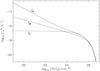 |
Fig. 1 CR ionisation rate as a function of the molecular hydrogen column density for the three models described in the text. |
In order to evaluate the ionisation rate along a field line, we average the contribution of
all the particles with different initial pitch angles over the solid angle
 (6)Finally,
to account for magnetic focusing, we multiply
(6)Finally,
to account for magnetic focusing, we multiply  by
χ. In the following, we choose as a “fiducial” spectrum the one
corresponding to the case k = ℳ and we neglect the subscript ℳ. Appendix
A shows the results for the other two models
k = ℒ,ℋ.
by
χ. In the following, we choose as a “fiducial” spectrum the one
corresponding to the case k = ℳ and we neglect the subscript ℳ. Appendix
A shows the results for the other two models
k = ℒ,ℋ.
3. Semi-analytic model
In PG11, we modelled molecular cloud cores as singular isothermal toroids, namely
scale-free, axisymmetric equilibrium configurations of an isothermal gas cloud under the
influence of self-gravity, gas pressure, and magnetic forces (Li & Shu 1996). These models are uniquely characterised by the
mass-to-flux ratio λ defined by
 (7)where G is
the gravitational constant, Φ the magnetic flux, and M(Φ) the mass
contained in the flux tube Φ. In this model the purely poloidal magnetic field threading the
core takes the form
(7)where G is
the gravitational constant, Φ the magnetic flux, and M(Φ) the mass
contained in the flux tube Φ. In this model the purely poloidal magnetic field threading the
core takes the form  (8)where
Φ(r,θ) is the magnetic flux function. Separation of variables requires
the equilibrium solution to take the self-similar form
(8)where
Φ(r,θ) is the magnetic flux function. Separation of variables requires
the equilibrium solution to take the self-similar form  (9)where
cs is the sound speed and
φ(θ) is a dimensionless function.
(9)where
cs is the sound speed and
φ(θ) is a dimensionless function.
If the core rotates with respect to the ambient medium, a toroidal component of the
magnetic field is expected to arise. We introduce a time-independent toroidal magnetic field
component by adding a term  (10)with
B0 constant to the magnetic field. This term is curl-free,
divergence-free, and scales as the poloidal component of the magnetic field. Additionally,
as (∇ × B) × B is unchanged by
this term, the equilibrium equations of the core are independent of the toroidal component
and, therefore, the solutions for the density and flux functions obtained by Li &
Shu (1996) remain formally valid. We are aware that,
in general, one does not expect the toroidal component of the field generated by the
rotation of the core to be curl-free. Nevertheless, it is very instructive to look at these
idealised configurations with the aim of disentangling column-density from magnetic-field
effects in the propagation of CR particles.
(10)with
B0 constant to the magnetic field. This term is curl-free,
divergence-free, and scales as the poloidal component of the magnetic field. Additionally,
as (∇ × B) × B is unchanged by
this term, the equilibrium equations of the core are independent of the toroidal component
and, therefore, the solutions for the density and flux functions obtained by Li &
Shu (1996) remain formally valid. We are aware that,
in general, one does not expect the toroidal component of the field generated by the
rotation of the core to be curl-free. Nevertheless, it is very instructive to look at these
idealised configurations with the aim of disentangling column-density from magnetic-field
effects in the propagation of CR particles.
Substitution of Eq. (9) into Eq. (8), and the addition of the toroidal component
(Eq. (10)) results in
![\begin{equation} \boldsymbol{B}(r,\theta) = \frac{4\pi c_{\rm s}^2 r}{G^{1/2}} \left[\frac{\ud\phi}{\ud\theta}\,\boldsymbol{\hat e}_r- \phi\,\boldsymbol{\hat e}_\theta+b_0\phi(\pi/2) \,\boldsymbol{\hat e}_\varphi\right] , \end{equation}](/articles/aa/full_html/2013/12/aa22407-13/aa22407-13-eq75.png) (11)where
(11)where
 (12)is
the ratio between the strength of the toroidal,
Bϕ, and the poloidal,
(12)is
the ratio between the strength of the toroidal,
Bϕ, and the poloidal,
 ,
field in the cloud’s midplane. Notice that the magnetic field diverges on the polar axis.
However, this is not a problem for our calculations, as the polar axis contains no mass.
,
field in the cloud’s midplane. Notice that the magnetic field diverges on the polar axis.
However, this is not a problem for our calculations, as the polar axis contains no mass.
The field lines that cross the midplane at
r = R0 and
ϕ = ϕ0, are then be given by  (13)and
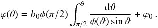 (14)As shown by Fig. 2, the magnetic field lines lie on the surfaces of nested
flux tubes defined by the condition Φ = const., and their twisting
increases as the distance from the axis of symmetry decreases.
(14)As shown by Fig. 2, the magnetic field lines lie on the surfaces of nested
flux tubes defined by the condition Φ = const., and their twisting
increases as the distance from the axis of symmetry decreases.
 |
Fig. 2 Magnetic field lines of the λ = 2.66 toroid with b0 = 0 (purely poloidal, upper plot), b0 = 1 (middle plot), and b0 = 10 (lower plot). Iso-density contours are shown in grey scales in unit of cm-3 in logarithmic scale, while the magnetic field module is shown in colour scale in unit of μG. Field line plots are generated using the visualisation software package MAYAVI (Ramachandran & Varoquaux 2011). |
3.1. Column-density versus magnetic-field effects on cosmic-ray ionisation rate
During the propagation of a CR, the ionisation rate decreases due to two main factors: (i) CRs lose energy, thus their capability of ionising hydrogen molecules, because of the increasing column density “seen” by the particles themselves (PGG09); (ii) magnetic mirroring reduces the ionisation rate more than magnetic focusing amplifies it (PG11). In order to distinguish the origin of the variation in the ionisation rate during the propagation, we assume several values for λ and b0 resulting in different density profiles and magnetic configurations.
We assume three different values for the mass-to-flux ratio (λ = 8.38,2.66, and 1.63) that acts modifying the density distribution as well as the pinching of the magnetic field lines. λ = 8.38 corresponds to the case of a “roundish” core, with a density distribution almost spherically symmetric; when λ = 1.63 the density is distributed in a disc-like configuration; finally, λ = 2.66 represents the intermediate case. The pinching of magnetic field lines increases for decreasing λ.
We start assuming b0 = 0 (purely poloidal field) whose effects on CR propagation are described in PG11, then we increase the toroidal field from b0 = 1 (poloidal and toroidal fields have comparable strengths) to b0 = 5,10, and 50. We follow the propagation of CRs entering the cloud from any direction with all possible initial pitch angles applying the method described in Sect. 2. With respect to PG11 we also consider the fact that the mirrored CRs can still ionise while propagating backwards. As expected, we find that this contribution to the ionisation is stronger in the outer part of the cloud, namely in the region also crossed by CRs which propagate backwards. This further ionisation is not crucial since these CRs have already passed through a large column density, losing their ionising power, but now it is included in the model. Figure 3 shows the order of magnitude of this contribution for the model ℳ: we plot the trend of the CR ionisation rate for a flux tube enclosing a mass of 1 M⊙ including all the contributions deriving from mirroring, focusing, and backward ionisation.
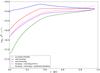 |
Fig. 3 Contributions to the ionisation rate as a function of the position along the symmetry axis for the model ℳ and a flux tube enclosing 1 M⊙. |
 |
Fig. 4 CR ionisation rate profiles for the model ℳ in the plane crossing the symmetry axis and perpendicular to the midplane (y = 0). The mass-to-flux ratio is λ = 2.66 and the strength of the toroidal field b0 increases from left to right. |
3.2. Dependence of ζH2 on the magnetic field configuration
In order to investigate on the effects of a given magnetic field configuration on the variations of ζH2, we assume a mass-to-flux ratio λ = 2.66 so that the density shape is fixed and we increase the magnitude of the toroidal component (Fig. 2). We find that increasing values of b0 correspond to a decrease of ζH2, in fact the area with low ionisation rate becomes larger and larger reflecting the signatures of the magnetic field configuration (Fig. 4). Since B ∝ (rsinθ)-1, the intensity of the magnetic field increases towards the symmetry axis. Therefore, the focusing factor becomes larger closer to the cloud’s axis, and this explains the increase of ζH2 in this region.
As b0 increases, the pitch angle α gets closer to π/2 quickly and the mirroring becomes more and more effective. However, as we know from PG11, increasing the toroidal component of B does not change significantly the relative importance of mirroring versus focusing effects, but it increases the effective column density as seen by a CR gyrating around the field. If this increase in N(H2) reaches the regime of exponential attenuation (N(H2) ≳ 1025 cm-2, see Fig. 1), the effect can be dramatic. However, this hardly happens in our semi-analytical model, which is taken as representative of a pc-scale clump of modest column density. Using profiles of density and magnetic field strength valid for smaller spatial scales taken from simulations of collapsing clouds, we will show that a reduction of ζH2 of orders of magnitude can be achieved (see Sect. 4).
Figure 5 shows a zoom in the central region at the core-size scale of 0.1 pc radius for the model ℳ in order to appreciate more explicitly the reduction in the ionisation rate: when the toroidal field is 50 times stronger than the poloidal field component, a value of ζH2 lower than the canonical value of 3 × 10-17 s-1 (≈10-16.5 s-1) is readily reached in the region close to the cloud’s midplane.
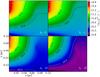 |
Fig. 5 CR ionisation rate maps for the model ℳ in the central 0.1 pc region in the plane y = 0 for λ = 2.66 and increasing b0. Black and white solid lines show the iso-ionisation rate contours. |
3.3. Dependence of ζH2 on the density profile
To examine the effects of the density configuration on the ionisation rate, we fix a value of the toroidal-to-poloidal ratio and we vary the mass-to-flux-ratio obtaining density profiles that span from a “roundish” core to a disc-like configuration (see Sect. 3.1). The effects of the column density can be promptly recognised by noticing that the ionisation rate profile follows the shape of the density profile. In Fig. 6 we superpose the iso-density contours to the ionisation rate maps. The regions where iso-density contours follow the ionisation rate profile reveal column-density effects. Conversely, the areas where the iso-density contours depart from the spatial distribution of ζH2 are representative of magnetic-field effects. In fact, for high values of λ the column density crossed is larger and ζH2 decreases rapidly (see PGG09). Said in a different way, in the λ = 8.38 model a particle “sees” a larger amount of N(H2) and it loses more energy than in the flatter λ = 1.63 model where the density along the field direction increases only close to the cloud’s midplane.
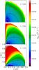 |
Fig. 6 CR ionisation rate maps for the model ℳ in the plane y = 0 for a fixed toroidal-to-poloidal ratio b0 = 10 and different values of the mass-to-flux-ratio. White and black contours represent the iso-density contours and the labels show log 10 [n/cm-3]. |
4. Numerical models
In this section we describe the ionisation rate maps obtained from a number of numerical
simulations related to a collapsing rotating core performed with the AMR code RAMSES1 (Teyssier 2002;
Fromang et al. 2006) and detailed in Joos et al.
(2012). They considered a spherical
1 M⊙ cloud with an initial density profile
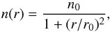 (15)\noindentwhere
n0 = 7.8 × 106 cm-3 and
r0 = 4.68 × 10⁻³ pc according to observations
(André et al. 2000; Belloche et al. 2002). The thermal-to-gravitational energy ratio is about
0.25 and the rotational-to-gravitational energy ratio is about 0.03. We select a series of
simulations from Joos et al. (2012) varying the
mass-to-flux ratio λ and the angle between the initial magnetic field
direction and the initial rotation axis αB,J.
Table 1 lists the parameters.
(15)\noindentwhere
n0 = 7.8 × 106 cm-3 and
r0 = 4.68 × 10⁻³ pc according to observations
(André et al. 2000; Belloche et al. 2002). The thermal-to-gravitational energy ratio is about
0.25 and the rotational-to-gravitational energy ratio is about 0.03. We select a series of
simulations from Joos et al. (2012) varying the
mass-to-flux ratio λ and the angle between the initial magnetic field
direction and the initial rotation axis αB,J.
Table 1 lists the parameters.
Parameters of the simulations described in the text (from Joos et al. 2012): mass-to-flux ratio, initial angle between the magnetic field direction and the rotation axis, time after the formation of the first Larson’s core (core formed in the centre of the pseudo-disc with n ≳ 1010 cm-3 and r ~ 10−20 AU), maximum mass of the protostellar core and of the disc. Last column gives information about the disc formation.
According to the method described in Sect. 2 we compute the ionisation rate maps making use of the model ℳ. For each case in Table 1, we show the maps of ζH2 in a plane parallel and perpendicular to the main direction of the magnetic field (always along the x axis) and containing the density peak, namely the (z,x) and the (y,z) plane, respectively. Besides, in Figs. 7−12 we plot the results for the whole computational domain (upper and middle left plots) and zooming into the inner 1000 AU (upper and middle right plots) plus a graph showing the magnetic field line morphology in the central 600 AU (lower plot).
We are aware of the fact that the ionisation rate should be computed simultaneously to the MHD model. This will be the subject of a future work, but the results described in this paper can be considered an important proof of concept that very low ionisation rate can be achieved in the inner regions of a collapsing cloud.
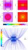 |
Fig. 7 CR ionisation maps and iso-density contours (black solid lines) for the case A1 in Table 1. Upper and middle left panels show the entire computational domain while upper and middle right panels show a zoom in the inner region. Upper panels show a slice of a plane parallel to the magnetic field direction, while middle panels refer to a slice of a perpendicular plane. Both planes contain the density peak and labels show log 10 [n/cm-3]. The lower plot shows the magnetic field line morphology in the central 600 AU of the RAMSES data cube. The colour bar shows the magnetic field module in Gauss units. |
4.1. Intermediate magnetisation (λ = 5)
We consider a couple of outputs (cases A1 and A2 in Table 1) for an aligned rotator (αB,J = 0) and super-critical cloud (λ = 5) in agreement with observations (Crutcher 1999). We choose two different times after the formation of the first Larson’s core in order to understand the effect of the tangling of magnetic field lines on CR propagation when a disc is not formed. Unlike the semi-analytical case (Sect. 3) where the density does not even achieve 105 cm-3 and the symmetry of the magnetic field configuration is conserved for any toroidal-to-poloidal ratio, in all the numerical models presented here the central density reaches the value of about 1013 cm-3 and in general it is higher than 1010 cm-3 in the inner 50−100 AU radius. Besides, the symmetry of magnetic field lines is broken very soon with time. This is likely due to the development of the interchange instability (Krasnopolsky et al. 2012).
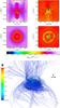 |
Fig. 8 CR ionisation maps and iso-density contours (black solid lines) for the case A2 in Table 1. See Fig. 7 for further information. |
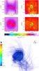 |
Fig. 9 CR ionisation maps and iso-density contours (black solid lines) for the case B in Table 1. See Fig. 7 for further information. |
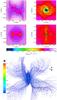 |
Fig. 10 CR ionisation maps and iso-density contours (black solid lines) for case C in Table 1. See Fig. 7 for further information. |
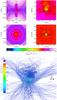 |
Fig. 11 CR ionisation maps and iso-density contours (black solid lines) for case D in Table 1. See Fig. 7 for further information. |
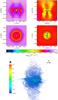 |
Fig. 12 CR ionisation maps and iso-density contours (black solid lines) for case E in Table 1. See Fig. 7 for further information. |
We know from the semi-analytical model (Sect. 3) that it is not possible to disentangle column-density from magnetic effects, but both intervene on the decrease of the ionisation rate. In Sect. 6 we give an estimate of the relative incidence of these two effects. As explained in Sect. 3.3, we can interpret the deviations between the iso-density contours and ζH2 maps as due to magnetic imprints. As an instance, in the upper right plot of Fig. 7 there is a clear departure between the contours at n = 109 cm-3 and the shape of the region where ζH2 reaches values of 2−3 × 10-18 s-1 (in yellow in the figure). Another example is the upper left plot of the same figure where the region in red with ζH2 ~ 1−2 × 10-17 s-1 extends for densities spanning from 105 to more than 107 cm-3 in a horizontal “strip” of about 5000 AU along the z axis. This calls to mind the magnetic field configuration (see lower panel of Fig. 7), in fact this is the region where field lines start to be twisted due to rotation. The middle right panel of Fig. 7 shows that less than 103 yr after the formation of the first Larson’s core, a central region with r ~ 100−200 AU is characterised by ζH2 ~ 2−4 × 10-18 s-1.
We compute ζH2 for a later-time configuration (case A2) with the same initial conditions (λ = 5, αB,J = 0). As previously mentioned, we lose the symmetry of field lines (see lower panel of Fig. 8) as well as of the density profile (see upper and middle right panels of Fig. 8). At large scales (upper and middle left plots), we notice that the region with ζH2 ≲ 10-17 s-1 is less extended along the z axis and it is elongated parallel to the x axis (i.e., parallel to the magnetic field). At small scales (upper and middle right plots), a flattened structure formed almost perpendicularly to the rotation axis can be noticed. In fact, even if the disc is not formed, the plane perpendicular to the rotation axis shows the presence of a “ring” with densities between 108 and 109 cm-3 and average ionisation rate of about 10-18 s-1 circumscribing the density peak up to a radius of about 300 AU.
We account for a configuration with the initial rotation axis twisted by π/4 towards the y axis, while the initial magnetic field direction is still along the x axis (case B in Table 1). This case predicts the formation of a disc with a flat rotation curve in the plane perpendicular to the rotation axis. In the central r ~ 50 AU region of both the (z,x) and the (y,z) plane, we find a CR ionisation rate lower than about 10-19 s-1. In the inner 500 AU region (upper and middle right panels of Fig. 9) we can still identify a relationship between ζH2 and n, even if the density profile becomes more and more irregular and field lines almost lose memory of their initial configuration (see lower panel of Fig. 9).
Finally, we consider the case of a perpendicular rotator (αB,J = π/2) so that initially the rotation axis is along the y axis. In this circumstance (case C in Table 1), a keplerian disc perpendicular to the rotation axis is predicted. Figure 10 shows this configuration, namely a face-on view in the (z,x) plane and an edge-on view of the disc in the (y,z) plane. It is worth noting in the face-on view (upper right panel of Fig. 10) a large region of r ~ 200 AU and n ≳ 109 cm-3 with ζH2 ≲ 10-18 s-1. Here the ratio between the toroidal component and the total magnetic field, Bϕ/|B |, is larger than about 0.4. We reach even lower values, with a minimum of 2 × 10-21 s-1 in the inner area that has an extent of a few tens of AU. The CR ionisation rate is so low that we can assume the gas to be effectively decoupled with the magnetic field. A similar behaviour can be also appreciated in the edge-on view (lower right panel of Fig. 10). The very low value of ζH2 found in this collapse region corresponds to the condition required by Mellon & Li (2009) for the formation of a 10 AU disc when λ = 4. However, we stress that in this case the formation of the disc is made possible by the misalignment of the angular momentum and the magnetic field of the cloud, whereas in the situation considered by Mellon & Li (2009) the two vectors are aligned and disc formation is enabled by the enhanced ambipolar diffusion resulting from the lower value of ζH2. Finally, the lower panel of Fig. 10 shows how the rotation perpendicular to the y axis forces the field lines (initially with a poloidal configuration along the x axis) to wrap around the rotation axis.
4.2. Strong magnetisation (λ = 2)
We analyse the case of an aligned rotator with strong magnetic field for a late-time configuration (case D of Table 1). A stronger field is more resistant to line twisting caused by rotation. In fact, in this case, the poloidal configuration can be still identified after about 6 kyr from the formation of the first Larson’s core (see lower panel of Fig. 11). As expected, the effect of magnetic braking is remarkable and the disc is not formed in the plane perpendicular to the rotation axis (see middle right panel of Fig. 11). In this case we find the ionisation rate to be more uniform and close to 10-17 s-1, while in the inner 50−100 AU ζH2 is of the order of 10-19 s-1 in the (z,x) plane and 10-18 s-1 in the (y,z) plane. Density contours in the (y,z) plane reveal high density fluctuations not allowing the formation of large high-density structures.
Since most molecular cloud cores appear to have significant levels of magnetisation (Crutcher 1999), this case is probably the most relevant for modelling cloud collapse. Our findings that the CR ionisation rate is one-two orders of magnitudes below the interstellar value in a region around the accreting protostar of radius ~50−100 AU, could indicate that a centrifugally supported disc of this size might form even in the strongly magnetised case. Of course, this question can only be answered by performing a fully self-consistent dynamical calculation of CR propagation during cloud collapse.
4.3. Weak magnetisation (λ = 17)
We model the case of weak magnetisation for an aligned rotator and we consider a late-time configuration (case E in Table 1). As shown in the lower panel of Fig. 12, since the magnetic field braking is very weak, rotation is able to strongly twist the field lines. It is interesting to notice how the contribution to the decrease of ζH2 is substantial perpendicularly to the disc plane. In fact, the upper right panel of Fig. 12 shows a large region along the x axis where ζH2 ≲ 10-18 s-1. This region is not limited to the high-density domain (n > 109 cm-3), but it broadens out along the rotation axis where the magnetic mirroring due to field line tangling up is very marked. As for case C (Sect. 4.1), the region with n ≳ 109 cm-3 and ζH2 ≲ 10-18 s-1 is characterised by Bϕ/|B| ≳ 0.4. In the (y,z) plane one can see the presence of the face-on disc and the rapid decrease of CR ionisation rate that reaches about 2 × 10-20 s-1 in the inner 1010 cm-3 iso-density contour. This is compatible with the results of Mellon & Li (2009) who find that a centrifugally supported disc of radius ~50 AU is formed by the collapse of a cloud with λ = 13.3, close to our value of 17, if ζH2 = 1 × 10-18 s-1, which is exactly the value that we find in this region. Again, the agreement found in this case may not be particularly significant, because in clouds characterised by an initially weak field, the magnetic braking may result inefficient regardless of the degree of ionisation of the gas. We stress again that, in order to draw firm conclusions on the role of CR ionisation in the resolution of the so-called “magnetic braking problem”, a fully self-consistent calculation including CR propagation and magnetic diffusion is required. In Sect. 6 we outline a procedure to include approximate treatment of CR transport in a MHD simulation.
5. Cosmic-ray ionisation rate at high column densities
The regime of high column densities,
N(H2) > 1025
cm-2, corresponding to surface mass densities Σ larger than a few g
cm-2, is interesting for applications to protoplanetary discs, where the
ionisation rate plays a major role in determining the “dead zones” where the generation of
turbulence by the magnetorotational instability is relatively inefficient (see e.g. Sano et
al. 2000; Okuzumi & Hirose 2011). In these applications, the CR ionisation rate is
usually assumed to be exponentially attenuated within the disc, with a decay length
Σ0 ≈ 96 g cm-2 (Umebayashi & Nakano 1981)2. Umebayashi & Nakano
(2009) propose an empirical formula for the CR
ionisation rate as a function of the depth from the disc surface, assuming a geometrically
thin disc and taking into account the fact that CRs penetrate the disc almost isotropically.
Their formula in cylindrical coordinates reads ![\begin{eqnarray} \label{un} \zeta^{\rm H_{2}}(r,z)&\approx&\frac{\zeta_{0}^{\rm H_{2}}}{2} \left\{\exp\left(-\frac{\Sigma^{+}(r,z)}{\Sigma_{0}}\right) \left[1+\left(\frac{\Sigma^{+}(r,z)}{\Sigma_{0}}\right)^{3/4}\right]^{-4/3} \right. \\\nonumber && \left. +\ \exp\left(-\frac{\Sigma^{-}(r,z)}{\Sigma_{0}}\right) \left[1+\left(\frac{\Sigma^{-}(r,z)}{\Sigma_{0}}\right)^{3/4}\right]^{-4/3}\right\}, \end{eqnarray}](/articles/aa/full_html/2013/12/aa22407-13/aa22407-13-eq168.png) (16)where
(16)where
 s-1 and Σ+ and Σ− are the vertical gas surface densities
measured from the upper (zup) and the lower boundary
(zlow) of the computational domain, respectively, namely
s-1 and Σ+ and Σ− are the vertical gas surface densities
measured from the upper (zup) and the lower boundary
(zlow) of the computational domain, respectively, namely
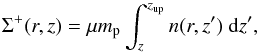 (17)and
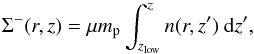 (18)where
mp is the proton mass and μ = 2.36 is the
molecular weight. We consider the numerical models described in Sect. 4 that allow the formation of a keplerian disc (case C and E in Table
1) comparing our CR ionisation rate maps with those
obtained by using Eq. (16).
(18)where
mp is the proton mass and μ = 2.36 is the
molecular weight. We consider the numerical models described in Sect. 4 that allow the formation of a keplerian disc (case C and E in Table
1) comparing our CR ionisation rate maps with those
obtained by using Eq. (16).
In order to make a consistent comparison, we let CRs propagate along straight lines without including magnetic effects, computing ζH2 using Eq. (5). This equation gives similar results to Eq. (16), the small variations being due to the difference in the assumed attenuation length (see left panels of Fig. 13). Nevertheless, the picture changes dramatically when considering the true path of CRs along the field lines with the inclusion of magnetic and focusing effects. In fact, the region with ζH2 < 10-18 s-1 grows considerably (see right panels of Fig. 13).
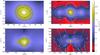 |
Fig. 13 Comparison between the CR ionisation rate distribution obtained by using the fitting formula (Eq. (16)) from Umebayashi & Nakano (2009) considering rectilinear propagation, black contours, and Eq. (5), white contours, for rectilinear propagation (left panels) and following the path of CRs along field lines with the inclusion of mirroring and focusing effects (right panels). The three concentric black contours in all the panels as well as the white contours in the left panels refer to log 10 (ζH2/s-1) = −17.5, −18, −21 going inwards. Labels are on a logarithmic scale and the colour coding shows the density distribution. Upper panels: model C; lower panels: model E of Table 1. |
This comparison represents the ultimate proof of the role of magnetic fields on CR propagation. Magnetic effects cannot be neglected since they set the extent to which CRs can determine the coupling between magnetic fields and the gas. In the next Section, we give a new fitting formula for ζH2 that accounts for the magnetic configuration.
6. Magnetic effects on the reduction of the CR ionisation rate: a useful fitting formula
In order to compare the relative importance of density and magnetic effects on the decrease of ζH2 in the central region of a core (n ≳ 109 cm-3), we let CRs propagate along field lines without accounting for mirroring and focusing, we refer to this setting as the “non-magnetic case”. This is easily done by following the path of CRs with initial pitch angle αICM = 0. According to Eq. (1), the pitch angle α during the propagation of the particle remains equal to zero. We generate CR ionisation maps as those presented in Figs. 7−12 and then we compute the quantity ℛ defined as the ratio between the rates obtained including and neglecting magnetic effects as in PG11.
We focus on cases C and E (see Table 1), corresponding to the cases where a keplerian disc is formed. In these models, the density reaches values larger than ~1010 cm-3 inside a region of a few 100 AU in size. Thus, one can be led to conclude that magnetic effects may be negligible since CRs have crossed a large column density so that the regime of exponential attenuation (N ≳ 1025 cm-2) is attained. On the contrary, we find that even at very high densities the role of magnetic fields in removing CRs and attenuating ζH2 is substantial. The results are shown in Fig. 14, where we plot the ratio ℛ of the CR ionisation rate computed keeping into account the evolution of the pitch angle to the same quantity computed in the non-magnetic case. We see that magnetic effects cause a net reduction of ζH2 of a factor of ~2 at large scales up to a factor of 3 to 10 in the inner regions.
We give a convenient fitting formula in order to reproduce the ionisation rate maps without
running the full code described in the paper. When in presence of a magnetic field, the
effective column density, Neff, seen by a CR can be much larger
than that obtained through a rectilinear propagation (see also Sect. 5): the more complex the morphology of the magnetic field, the larger is
the path covered by a charged particle. If N(H2) is the average
column density seen by an isotropic flux of CRs, Neff has the
form  (19)The factor ℱ depends on
the ratio between the toroidal and the poloidal components of the magnetic field,
b = |Bϕ/Bp |,
as well as on its module. It reads
(19)The factor ℱ depends on
the ratio between the toroidal and the poloidal components of the magnetic field,
b = |Bϕ/Bp |,
as well as on its module. It reads  (20)where
  (21)bminand
bmax being the minimum and the maximum value of
b in the whole data cube, respectively. When the magnetic field strength
is negligible, CRs propagate along straight lines. In this case ℱ = 0 and
Neff = N(H2), otherwise
ℱ > 0 and
Neff > N(H2).
Comparing the column density seen by a CR evaluated with our code and with Eq. (19), we find that it is safe to approximate the
poloidal configuration to a rectilinear path. This explains why we introduce the dependence
of ℱ on b∗. In fact, b∗ varies
between 0 and 1, being equal to 0 for a purely poloidal configuration. We also find that the
higher the density, the stronger is the role of the magnetic field in increasing
Neff. This justifies the presence in Eq. (19) of the power s that reads
(21)bminand
bmax being the minimum and the maximum value of
b in the whole data cube, respectively. When the magnetic field strength
is negligible, CRs propagate along straight lines. In this case ℱ = 0 and
Neff = N(H2), otherwise
ℱ > 0 and
Neff > N(H2).
Comparing the column density seen by a CR evaluated with our code and with Eq. (19), we find that it is safe to approximate the
poloidal configuration to a rectilinear path. This explains why we introduce the dependence
of ℱ on b∗. In fact, b∗ varies
between 0 and 1, being equal to 0 for a purely poloidal configuration. We also find that the
higher the density, the stronger is the role of the magnetic field in increasing
Neff. This justifies the presence in Eq. (19) of the power s that reads
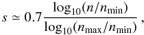 (22)nminand
nmax being the minimum and the maximum value of the density in
the whole data cube, respectively. The factor 0.7 in Eq. (22) has been introduced to reproduce the CR ionisation maps in the upper
and middle panels of Figs. 7−12. Notice also that the factor ℱ depends on the local value of the
magnetic field, since b and | B | are
computed in a given point, but it also accounts for the large scale configuration by means
of b∗ and s.
(22)nminand
nmax being the minimum and the maximum value of the density in
the whole data cube, respectively. The factor 0.7 in Eq. (22) has been introduced to reproduce the CR ionisation maps in the upper
and middle panels of Figs. 7−12. Notice also that the factor ℱ depends on the local value of the
magnetic field, since b and | B | are
computed in a given point, but it also accounts for the large scale configuration by means
of b∗ and s.
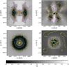 |
Fig. 14 Maps of the ratio ℛ between the CR ionisation rates in the magnetic and non-magnetic case for the case E in Table 1. Left panels show the entire computational domain while right panels show a zoom in the inner region. Upper panels show a slice of a plane parallel to the magnetic field direction, while lower panels refer to a slice of a perpendicular plane. Iso-contours of ℛ are shown in cyan (ℛ = 0.1), yellow (ℛ = 0.3), orange (ℛ = 0.5), and purple (ℛ = 0.7). |
Once evaluated the effective column density, the corresponding (effective) CR ionisation
rate,  ,
is obtained by
,
is obtained by  (23)where
ζH2(Neff) is computed
using Eq. (5) after replacing
N(α) and Σ(α) with
Neff and
μmHNeff,
respectively. The factor κ is given by
(23)where
ζH2(Neff) is computed
using Eq. (5) after replacing
N(α) and Σ(α) with
Neff and
μmHNeff,
respectively. The factor κ is given by  (24)and
it represents the correction for magnetic effects. Equation (23) gives a correct result within a factor of 3 and it holds for
magnetic field strengths smaller than about 1 G. It can be very helpful for non-ideal MHD
simulations so as to compute diffusion coefficients and it can be also implemented in
chemical models in order to have a more precise description of the observational results.
Figure 15 shows the goodness of the fit for the inner
region of case C in Table 1.
(24)and
it represents the correction for magnetic effects. Equation (23) gives a correct result within a factor of 3 and it holds for
magnetic field strengths smaller than about 1 G. It can be very helpful for non-ideal MHD
simulations so as to compute diffusion coefficients and it can be also implemented in
chemical models in order to have a more precise description of the observational results.
Figure 15 shows the goodness of the fit for the inner
region of case C in Table 1.
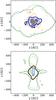 |
Fig. 15 Comparison between the CR ionisation rate evaluated with the code described in the paper, solid contours, and with Eq. (23), dashed contours for the case C in Table 1. The grey shaded area shows the region where the difference among contours is larger than a factor of 3 and the black solid contour refers to the region where | B| = 1 G. Green, orange, blue, cyan, and red contours are related to log 10(ζH2/s-1) = −17, −17.5, −18, −19, and −20, respectively. |
7. Conclusions
In this study we explored the distribution of the CR ionisation rate in molecular clouds, examining and extending the results obtained in PGG09 and PG11. We employed a semi-analytical model in order to understand when the variations of ζH2 can be attributed to energy losses due to the increasing column density passed through or to magnetic mirroring and focusing. The main conclusion is that an increment of the toroidal component, and in general a more tangled magnetic field, corresponds to a decrease of ζH2 because of the growing preponderance of mirroring over focusing. That is to say, large variations of the direction of field lines cause a rapid increase of the cosmic-ray pitch angle towards the mirroring angle. Conversely, fixing a magnetic field line configuration while varying the density profile allowed us to identify the weakening of the ionisation power caused by energy losses. As expected, moving from a “roundish” core towards a disc-like configuration, the distribution of ζH2 follows the density profile shape.
In the second part of the paper we analysed a number of numerical simulation outputs related to a rotating collapsing core following the propagation of cosmic rays at different time steps, varying the degree of magnetisation and the initial orientation of the main magnetic field direction with respect to the rotation axis. Being aware of the fact that the correct manner of dealing with CR propagation should be computing their distribution simultaneously with the MHD simulation, we believe that our conclusions represent an important proof of concept. In particular, in the central 100 AU region, the number density is higher than 1010 cm-3 and a H2 column density larger than 1025 cm-2 is promptly reached. This actually means entering the exponential attenuation regime where the CR ionisation rate is independent of the CR spectrum assumed and drops below 10-18 s-1. However, we prove that even in the high-density region, the presence of a magnetic field can reduce ζH2 up to a factor larger than 10. As for the semi-analytical model, we also conclude that the morphology of the ζH2 maps depends both on the density profile and on the magnetic field line configuration.
Finally we focused on the morphology of ζH2 in the inner region where a Keplerian disc is formed. We found that the inclusion of magnetic field effects in the calculation of ζH2 brings to the formation of a large central region of 100 to 200 AU where the CR ionisation rate is well below the ordinarily used value of 10-17 s-1. This provides support to the hypothesis of Mellon & Li (2009) according to which the magnetic braking efficiency can be reduced if ζH2 ≲ 10-18 s-1 allowing the formation of the disc. In order to test this hypothesis a self-consistent MHD collapse calculation including CR propagation is needed.
We compared our results with those obtained by Umebayashi & Nakano (2009) in the case of an unmagnetised disc, showing that the exclusion of CRs resulting from magnetic mirroring deeply affects the CR ionisation rate pattern in the collapse region. To account for the effects of the magnetic configuration, we formulated a general fitting expression to approximately compute ζH2 as a function of the column density, magnetic field strength, and toroidal-to-poloidal magnetic field ratio. This empirical expression reproduces quite accurately our numerical results.
Non-ideal MHD models predict that magnetic braking becomes inefficient at densities n > 1012 cm-3, when magnetic field diffusion becomes faster than the dynamical evolution (Dapp et al. 2012). In our models we observe that the drop in ζH2 takes place in some cases even at lower densities (n > 109 cm-3), resulting in very low ionisation fractions. The consequences of the reduced CR ionisation rate on the magnetic diffusion coefficients (ambipolar, Hall, and Ohm) will be the subject in a forthcoming paper.
RAMSES simulations were analysed using PyMSES (Labadens et al. 2011).
The calculations of PGG09 and PGG13 suggest however that the attenuation length for protons may be a factor of ~2 larger than that derived by Umebayashi & Nakano (1981).
Acknowledgments
M.P. thanks Marc Joos and Andrea Ciardi for their help in accessing RAMSES simulations and Natalia Dzyurkevich for illuminating discussions about ionisation in discs. M.P. and P.H. acknowledge the financial support of the Agence Nationale pour la Recherche (ANR) through the COSMIS project.
References
- Allen, F. C., Li, Z.-Y., & Shu, F. H. 2003, ApJ, 599, 363 [NASA ADS] [CrossRef] [Google Scholar]
- André, P., Ward-Thompson, D., & Barsony, M. 2000, Protostars and Planets IV, 59 [Google Scholar]
- Belloche, A., André, P., Despois, D., et al. 2002, A&A, 393, 927 [Google Scholar]
- Braiding, C. R., & Wardle, M. 2012a, MNRAS, 422, 261 [NASA ADS] [CrossRef] [Google Scholar]
- Braiding, C. R., & Wardle, M. 2012b, MNRAS, 427, 3188 [NASA ADS] [CrossRef] [Google Scholar]
- Ceccarelli, C., Hily-Blant, P., Montmerle, T., et al. 2011, ApJ, 740, L4 [Google Scholar]
- Cesarsky, C. J., & Völk, H. J. 1978, A&A, 70, 367 [NASA ADS] [Google Scholar]
- Chandran, B. D. G. 2000, ApJ, 529, 513 [NASA ADS] [CrossRef] [Google Scholar]
- Crapsi, A., Caselli, P., Walmsley, C. M., et al. 2007, A&A, 470, 221 [NASA ADS] [CrossRef] [EDP Sciences] [Google Scholar]
- Crutcher, R. M. 1999, ApJ, 520, 706 [NASA ADS] [CrossRef] [Google Scholar]
- Dapp, W. B., & Basu, S. 2010, A&A, 521, L56 [NASA ADS] [CrossRef] [EDP Sciences] [Google Scholar]
- Dapp, W. B., Basu, S., & Kunz, M. W. 2012, A&A, 541, A35 [NASA ADS] [CrossRef] [EDP Sciences] [Google Scholar]
- Desch, S. J., Connolly, H. C., Jr., & Srinivasan, G. 2004, ApJ, 602, 528 [NASA ADS] [CrossRef] [MathSciNet] [Google Scholar]
- Draine, B. T., & Sutin, B. 1987, ApJ, 320, 803 [NASA ADS] [CrossRef] [Google Scholar]
- Fromang, S., Hennebelle, P., & Teyssier, R. 2006, A&A, 457, 371 [NASA ADS] [CrossRef] [EDP Sciences] [Google Scholar]
- Galli, D., Lizano, S., Shu, F. H., & Allen, A. 2006, ApJ, 647, 374 [NASA ADS] [CrossRef] [Google Scholar]
- Gerin, M., De Luca, M., Black, J., et al. 2010, A&A, 518, L110 [NASA ADS] [CrossRef] [EDP Sciences] [Google Scholar]
- Hartquist, T. W., Doyle, H. T., & Dalgarno, A. 1978, A&A, 68, 65 [NASA ADS] [Google Scholar]
- Hennebelle, P., & Ciardi, A. 2009, A&A, 506, L29 [NASA ADS] [CrossRef] [EDP Sciences] [Google Scholar]
- Hennebelle, P., & Fromang, S. 2008, A&A, 477, 9 [NASA ADS] [CrossRef] [EDP Sciences] [Google Scholar]
- Indriolo, N., & McCall, B. J. 2012, ApJ, 745, 91 [NASA ADS] [CrossRef] [Google Scholar]
- Joos, M., Hennebelle, P., & Ciardi, A. 2012, A&A, 543, A128 [NASA ADS] [CrossRef] [EDP Sciences] [Google Scholar]
- Krasnopolsky, R., Li, Z.-Y., & Shang, H. 2011, ApJ, 733, 54 [NASA ADS] [CrossRef] [Google Scholar]
- Krasnopolsky, R., Li, Z.-Y., & Shang, H., et al. 2012 ApJ, 757, 77 [CrossRef] [Google Scholar]
- Labadens, M., Chapon, D., Pomaréde, D., et al. 2011, ADASS XXI Proc., 461, 837 [Google Scholar]
- Li, Z.-Y., & Shu, F. H. 1996, ApJ, 472, 211 [NASA ADS] [CrossRef] [Google Scholar]
- Machida, M. N., Inutsuka, S.-I., & Matsumoto, T. 2011, PASJ, 63, 555 [NASA ADS] [CrossRef] [Google Scholar]
- McCall, B. J., Geballe, T. R., Hinke, K. H., et al. 1998, Science, 279, 1910 [NASA ADS] [CrossRef] [PubMed] [Google Scholar]
- McCall, B. J., Huneycutt, A. J., Saykally, R. J., et al. 2003, Nature, 422, 500 [NASA ADS] [CrossRef] [PubMed] [Google Scholar]
- Mellon, R. R., & Li, Z.-H. 2008, ApJ, 681, 1356 [NASA ADS] [CrossRef] [Google Scholar]
- Mellon, R. R., & Li, Z.-H. 2009, ApJ, 698, 922 [NASA ADS] [CrossRef] [Google Scholar]
- Meneguzzi, M., Adouze, J., & Reeves, H. 1971, A&A, 15, 377 [Google Scholar]
- Montmerle, T. 2010, in High Energy Phenomena in Massive Stars, eds. J. Martí, P. L. Luque-Escamilla, & J. A. Combi (San Francisco, CA: ASP), ASP Conf. Ser., 422, 85 [Google Scholar]
- Nakano, T. 1984, Fund. Cosmic Phys., 9, 139 [NASA ADS] [Google Scholar]
- Neufeld, D. A., Goicoechea, J. R., Sonnentrucker, P., et al. 2010, A&A, 521, L10 [NASA ADS] [CrossRef] [EDP Sciences] [Google Scholar]
- Okuzumi, S., & Hirose, S., ApJ, 742, 65 [Google Scholar]
- Padoan, P., & Scalo, 2005, ApJ, 624, L97 [NASA ADS] [CrossRef] [Google Scholar]
- Padovani, M., Galli, D., & Glassgold, A. E. 2009, A&A, 501, 619 (PGG09) [NASA ADS] [CrossRef] [EDP Sciences] [Google Scholar]
- Padovani, M., & Galli, D. 2011, A&A, 530, A109 (PG11) [NASA ADS] [CrossRef] [EDP Sciences] [Google Scholar]
- Padovani, M., Galli, D., & Glassgold, A. E. 2013, A&A, 549, C3 (PGG13) [NASA ADS] [CrossRef] [EDP Sciences] [Google Scholar]
- Ramachandran, P., & Varoquaux, G. 2011, IEEE Comput. Sci Eng., 13, 40 [Google Scholar]
- Rimmer, P. B., Herbst, E., Morata, O., et al. 2012, A&A, 537, A7 [NASA ADS] [CrossRef] [EDP Sciences] [Google Scholar]
- Sano, T., Miyama, S. M., Umebayashi, T., et al. 2000, ApJ, 543, 486 [NASA ADS] [CrossRef] [Google Scholar]
- Santos-Lima, R., de Gouveia Dal Pino, E. M., & Lazarian, A. 2013, MNRAS, 429, 3371 [NASA ADS] [CrossRef] [Google Scholar]
- Seifried, D., Banerjee, R., Pudritz, R. E., et al. 2012, MNRAS, 423, 40 [Google Scholar]
- Shu, F. H., Galli, D., Lizano, S., & Cai, M. 2006, ApJ, 647, 382 [NASA ADS] [CrossRef] [Google Scholar]
- Skilling, J., & Strong, A. W. 1976, A&A, 53, 253 [NASA ADS] [Google Scholar]
- Takayanagi, M. 1973, PASJ, 25, 327 [NASA ADS] [Google Scholar]
- Teyssier, R. 2002, A&A, 385, 337 [NASA ADS] [CrossRef] [EDP Sciences] [Google Scholar]
- Umebayashi, T., & Nakano, T. 1981, PASJ, 33, 617 [NASA ADS] [Google Scholar]
- Umebayashi, T., & Nakano, T. 2009, ApJ, 690, 69 [NASA ADS] [CrossRef] [Google Scholar]
Appendix A: Models ℒ and ℋ
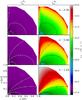 |
Fig. A.1 CR ionisation rate maps for the model ℒ (left column) and ℋ (right column) in the plane y = 0 for a fixed toroidal-to-poloidal ratio b0 = 10 and different values of the mass-to-flux-ratio. White and black contours represent the iso-density contours and the labels show log 10 [n/cm-3]. |
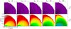 |
Fig. A.2 CR ionisation rate profiles for the model ℒ (top row) and ℋ (bottom row) in the plane crossing the symmetry axis and perpendicular to the midplane (y = 0). The mass-to-flux ratio is λ = 2.66 and the strength of the toroidal field b0 increases from left to right. |
For the sake of completeness, we show the CR ionisation rate
 obtained adopting the spectra corresponding to the cases k = ℒ and
k = ℋ in Fig. 1. These represent
two extreme behaviours of CR ionisation as a function of column density. For both cases,
we compute the dependence of
on the density profile and the magnetic field configuration for the semi-analytical cloud
models described in Sect. 3. In particular we show
results for λ = 8.38,2.66, and 1.63 with
b0 = 10 (Fig. A.1) and
for λ = 2.66 with
b0 = 0,1,5,10,
and 50 (Fig. A.2). As expected, the CR ionisation
rate for the case k = ℒ is independent of the value of the mass-to-flux
ratio and the toroidal-to-poloidal ratio since the exponential regime
(N(H2) ≳ 1025 cm-2) is not attained
and
obtained adopting the spectra corresponding to the cases k = ℒ and
k = ℋ in Fig. 1. These represent
two extreme behaviours of CR ionisation as a function of column density. For both cases,
we compute the dependence of
on the density profile and the magnetic field configuration for the semi-analytical cloud
models described in Sect. 3. In particular we show
results for λ = 8.38,2.66, and 1.63 with
b0 = 10 (Fig. A.1) and
for λ = 2.66 with
b0 = 0,1,5,10,
and 50 (Fig. A.2). As expected, the CR ionisation
rate for the case k = ℒ is independent of the value of the mass-to-flux
ratio and the toroidal-to-poloidal ratio since the exponential regime
(N(H2) ≳ 1025 cm-2) is not attained
and  is substantially independent of the column density.
On the other hand, the CR ionisation rate for the model ℋ is comparable with that of the
model ℳ described in the main text. However, as shown in Fig. A.2, even when the toroidal field is strong
(b0 = 50), in the inner region of the toroid below 0.1 pc,
 is of the order of 10-16 s-1, about one order of magnitude higher
than the values estimated from observations. For this reason, the model ℳ has been chosen
as the fiducial model.
is of the order of 10-16 s-1, about one order of magnitude higher
than the values estimated from observations. For this reason, the model ℳ has been chosen
as the fiducial model.
All Tables
Parameters of the simulations described in the text (from Joos et al. 2012): mass-to-flux ratio, initial angle between the magnetic field direction and the rotation axis, time after the formation of the first Larson’s core (core formed in the centre of the pseudo-disc with n ≳ 1010 cm-3 and r ~ 10−20 AU), maximum mass of the protostellar core and of the disc. Last column gives information about the disc formation.
All Figures
|
Fig. 1 CR ionisation rate as a function of the molecular hydrogen column density for the three models described in the text. |
| In the text | |
|
Fig. 2 Magnetic field lines of the λ = 2.66 toroid with b0 = 0 (purely poloidal, upper plot), b0 = 1 (middle plot), and b0 = 10 (lower plot). Iso-density contours are shown in grey scales in unit of cm-3 in logarithmic scale, while the magnetic field module is shown in colour scale in unit of μG. Field line plots are generated using the visualisation software package MAYAVI (Ramachandran & Varoquaux 2011). |
| In the text | |
|
Fig. 3 Contributions to the ionisation rate as a function of the position along the symmetry axis for the model ℳ and a flux tube enclosing 1 M⊙. |
| In the text | |
|
Fig. 4 CR ionisation rate profiles for the model ℳ in the plane crossing the symmetry axis and perpendicular to the midplane (y = 0). The mass-to-flux ratio is λ = 2.66 and the strength of the toroidal field b0 increases from left to right. |
| In the text | |
|
Fig. 5 CR ionisation rate maps for the model ℳ in the central 0.1 pc region in the plane y = 0 for λ = 2.66 and increasing b0. Black and white solid lines show the iso-ionisation rate contours. |
| In the text | |
|
Fig. 6 CR ionisation rate maps for the model ℳ in the plane y = 0 for a fixed toroidal-to-poloidal ratio b0 = 10 and different values of the mass-to-flux-ratio. White and black contours represent the iso-density contours and the labels show log 10 [n/cm-3]. |
| In the text | |
|
Fig. 7 CR ionisation maps and iso-density contours (black solid lines) for the case A1 in Table 1. Upper and middle left panels show the entire computational domain while upper and middle right panels show a zoom in the inner region. Upper panels show a slice of a plane parallel to the magnetic field direction, while middle panels refer to a slice of a perpendicular plane. Both planes contain the density peak and labels show log 10 [n/cm-3]. The lower plot shows the magnetic field line morphology in the central 600 AU of the RAMSES data cube. The colour bar shows the magnetic field module in Gauss units. |
| In the text | |
|
Fig. 8 CR ionisation maps and iso-density contours (black solid lines) for the case A2 in Table 1. See Fig. 7 for further information. |
| In the text | |
|
Fig. 9 CR ionisation maps and iso-density contours (black solid lines) for the case B in Table 1. See Fig. 7 for further information. |
| In the text | |
|
Fig. 10 CR ionisation maps and iso-density contours (black solid lines) for case C in Table 1. See Fig. 7 for further information. |
| In the text | |
|
Fig. 11 CR ionisation maps and iso-density contours (black solid lines) for case D in Table 1. See Fig. 7 for further information. |
| In the text | |
|
Fig. 12 CR ionisation maps and iso-density contours (black solid lines) for case E in Table 1. See Fig. 7 for further information. |
| In the text | |
|
Fig. 13 Comparison between the CR ionisation rate distribution obtained by using the fitting formula (Eq. (16)) from Umebayashi & Nakano (2009) considering rectilinear propagation, black contours, and Eq. (5), white contours, for rectilinear propagation (left panels) and following the path of CRs along field lines with the inclusion of mirroring and focusing effects (right panels). The three concentric black contours in all the panels as well as the white contours in the left panels refer to log 10 (ζH2/s-1) = −17.5, −18, −21 going inwards. Labels are on a logarithmic scale and the colour coding shows the density distribution. Upper panels: model C; lower panels: model E of Table 1. |
| In the text | |
|
Fig. 14 Maps of the ratio ℛ between the CR ionisation rates in the magnetic and non-magnetic case for the case E in Table 1. Left panels show the entire computational domain while right panels show a zoom in the inner region. Upper panels show a slice of a plane parallel to the magnetic field direction, while lower panels refer to a slice of a perpendicular plane. Iso-contours of ℛ are shown in cyan (ℛ = 0.1), yellow (ℛ = 0.3), orange (ℛ = 0.5), and purple (ℛ = 0.7). |
| In the text | |
|
Fig. 15 Comparison between the CR ionisation rate evaluated with the code described in the paper, solid contours, and with Eq. (23), dashed contours for the case C in Table 1. The grey shaded area shows the region where the difference among contours is larger than a factor of 3 and the black solid contour refers to the region where | B| = 1 G. Green, orange, blue, cyan, and red contours are related to log 10(ζH2/s-1) = −17, −17.5, −18, −19, and −20, respectively. |
| In the text | |
|
Fig. A.1 CR ionisation rate maps for the model ℒ (left column) and ℋ (right column) in the plane y = 0 for a fixed toroidal-to-poloidal ratio b0 = 10 and different values of the mass-to-flux-ratio. White and black contours represent the iso-density contours and the labels show log 10 [n/cm-3]. |
| In the text | |
|
Fig. A.2 CR ionisation rate profiles for the model ℒ (top row) and ℋ (bottom row) in the plane crossing the symmetry axis and perpendicular to the midplane (y = 0). The mass-to-flux ratio is λ = 2.66 and the strength of the toroidal field b0 increases from left to right. |
| In the text | |
Current usage metrics show cumulative count of Article Views (full-text article views including HTML views, PDF and ePub downloads, according to the available data) and Abstracts Views on Vision4Press platform.
Data correspond to usage on the plateform after 2015. The current usage metrics is available 48-96 hours after online publication and is updated daily on week days.
Initial download of the metrics may take a while.