| Issue |
A&A
Volume 560, December 2013
|
|
|---|---|---|
| Article Number | A31 | |
| Number of page(s) | 7 | |
| Section | The Sun | |
| DOI | https://doi.org/10.1051/0004-6361/201322396 | |
| Published online | 02 December 2013 | |
Excitation of an outflow from the lower solar atmosphere and a co-temporal EUV transient brightening⋆
1
Armagh Observatory,
College Hill,
Armagh
BT61 9DG,
UK
e-mail:
This email address is being protected from spambots. You need JavaScript enabled to view it.
2
School of Mathematics and Statistics, University of
Sheffield, Hicks Building,
Hounsfield Road, Sheffield
S3 7RH,
UK
Received: 30 July 2013
Accepted: 30 October 2013
Abstract
Aims. We analyse an absorption event within the Hα line wings, which has been identified as a surge, and the co-spatial evolution of an EUV brightening, with spatial and temporal scales analogous to a small blinker.
Methods. We conduct a multi-wavelength, multi-instrument analysis using high-cadence, high-resolution data, collected by the Interferometric BIdimensional Spectrometer on the Dunn Solar Telescope, as well as the space-borne Atmospheric Imaging Assembly and Helioseismic and Magnetic Imager instruments on board the Solar Dynamics Observatory.
Results. One large absorption event situated within the plage region trailing the lead sunspot of AR 11579 is identified within the Hα line wings. This event is found to be co-spatially linked to a medium-scale (around 4′′ in diameter) brightening within the transition region and corona. This ejection appears to have a parabolic evolution, first forming in the Hα blue wing before fading and reappearing in the Hα red wing, and comprises a number of smaller fibril events. The line-of-sight photospheric magnetic field shows no evidence of cancellation leading to this event.
Conclusions. Our research has identified clear evidence that at least a subset of transient brightening events in the transition region is linked to the influx of cooler plasma from the lower solar atmosphere during large eruptive events, such as surges. These observations agree with previous numerical researches on the nature of blinkers and, therefore, suggest that magnetic reconnection is the driver of the analysed surge events; however, further research is required to confirm this.
Key words: Sun: photosphere / Sun: chromosphere / Sun: transition region / Sun: corona
A movie attached to Fig. 2 is available in electronic form at http://www.aanda.org
© ESO, 2013
1. Introduction
The solar atmosphere is a dynamic environment that has been observed to ubiquitously change on ever smaller scales with the advancement of observational techniques. The complex interactions between the strong, inferred magnetic fields and plasma flows are believed to lead to the formation of a number of structures that are easily identified from the photosphere to the corona (e.g., spicules, macro-spicules, surges, coronal loops, prominences). Many such solar structures have been widely studied in recent years, thanks to their assumed influence in heating the corona to multi-million Kelvin temperatures.
Blinkers, both small-scale (often between 3′′ and 10′′ in diameter) and short-lived (less than 20 min) brightening events, have been extensively researched in the past two decades owing to their dynamic nature. First observed with the Coronal Diagnostic Spectrometer (CDS; described by Harrison et al. 1995) instrument, on board the Solar and Heliospheric Observatory (SOHO), blinkers are often discussed with respect to chromospheric and coronal extreme UV (EUV) lines (see, for example, Harrison 1997; Berghmans et al. 1998; Doyle et al. 2004). The nature of these transient brightenings in the EUV was analysed by Harrison et al. (1999), who hypothesized that blinkers in the upper atmosphere were caused by an increase in density or filling factor, rather than by a localized temperature enhancement (a result supported by, e.g., Teriaca et al. 2001; Bewsher et al. 2003; Madjarska & Doyle 2003).
Combining SOHO/CDS observations with magnetograms inferred using the Michelson Doppler Imager (MDI; Scherrer et al. 1995) instrument, Bewsher et al. (2002) and Parnell et al. (2002) analysed the links between blinkers and the underlying photospheric magnetic field within the quiet Sun (QS) and active regions (AR), respectively. It was found that a high proportion of blinkers (approximately 75%) occurred co-spatially to strong uni-polar fields, so it was inferred that magnetic reconnection within the upper atmosphere was unlikely to be the driver of these events. These results agreed with the interpretations of Priest et al. (2002), who suggested that the forced interactions of cooler plasma from the lower solar atmosphere and warmer transition region plasma through a driver in the photosphere could lead to the formation of blinkers due to density enhancements. Indeed, five specific scenarios were discussed, and a cartoon was presented that detailed each of the proposed mechanisms.
Within QS research, it has often been reported that there is rarely a signature of blinker events within coronal lines (see, e.g., Harrison 1997; Bewsher et al. 2002; Madjarska & Doyle 2003). A study of AR events, however, by Parnell et al. (2002) found that a significant number of blinkers were co-spatial to intensity enhancements in coronal lines (such as the Mg ix and Mg x ions, which sample plasma at approximately 106). It was hypothesized that the increased intensity within these lines corresponded to the higher background emission of the corona within ARs and that, therefore, higher sensitivity within the QS may return similar results. Indeed, more recent work by Madjarska et al. (2009) and Subramanian et al. (2012) shows that the term blinker covers a range of phenomena with blinkers originating at both chromospheric, transition region and coronal heights.
One suggested mechanism (see Priest et al. 2002) by which blinkers could be formed is by the ejection of cool plasma into the upper atmosphere (potentially manifesting as, e.g., spicules). An example of a larger scale eruptive phenomena observed to propagate from the lower solar atmosphere into the transition region and corona are solar surges. These events have been observed for several decades (see, for example, Roy 1973b,a, and references therein) and manifest as long, thin, dark jets in the Hα line wings, often associated with transition region and coronal brightenings (e.g., Jiang et al. 2007; Madjarska et al. 2009; Kayshap et al. 2013). Due to the strong correlation between surge formation and strong, opposite polarity field regions, it has been widely suggested that these events are formed through magnetic reconnection in the lower atmosphere. Yokoyama & Shibata (1996) performed numerical simulations of the solar atmosphere, finding evidence of both slow shocks and plasma ejections, analogous to surges, away from a magnetic reconnection site leading to simultaneous X-ray brightenings and Hα surge flows.
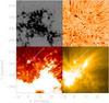 |
Fig. 1 Snapshot of data used in this study at 17:30:01 UT. (Top left) SDO/HMI, (Top right) Hα blue wing, (Bottom left) SDO/AIA 304 Å, and (Bottom right) SDO/AIA 171 Å. The plotted arrow indicates the event which we discuss in this article. |
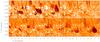 |
Fig. 2 Temporal evolution in the blue and red wings of the Hα line profile. (Top row) Evolution of this event through time (from 17:29:42 UT to 17:35:35 UT) in the blue wing (each frame is separated by approximately 70 s). (Bottom row) Corresponding FOV and frames in the red wing showing the apparent parabolic trajectory of this event. The white line indicates an artificial slit used to enable a time-distance plot (shown in Fig. 3). |
Due to the many similarities in morphology, a concerted effort has been made in recent years to test whether eruptive events, such as surges or macro-spicules, and blinker phenomena, are linked. O’Shea et al. (2005) analysed data at the limb and found events analogous to blinkers occurring co-spatially to regions of dynamic motions, including the ejection of cool photospheric plasma through spicules. It was suggested that the most likely cause of blinkers was the heating of spicular mass within the upper-atmosphere. This work was continued by Madjarska et al. (2006), who studied lightcurves from two on disc blinkers and one limb event finding comparable evolutions through time. To fully understand this link, Priest et al. (2002) suggested co-spatial and co-temporal Hα and EUV observations (such as the He ii ion) would be required.
The results in this article are obtained using high-resolution, high-cadence data from both ground-based and space-borne instruments to analyse the formation of a single event in the Hα line wings, which is co-spatial with a brightening at EUV wavelengths in both the transition region and the corona. We format our research as follows: in Sect. 2, we discuss the observations used in this article and Sect. 3 presents the results of our analysis. Finally, we make a short discussion of the implications of this study in Sect. 4.
2. Observations
In this article, co-temporal datasets from three instruments are analysed. We make use of ground-based data collected using the Interferometric BIdimensional Spectrometer (IBIS; Cavallini et al. 2000) instrument situated at the National Solar Observatory, New Mexico. These data were collected during a period of good seeing on the 30 September 2012 between 17:22:02 UT and 17:37:06 UT and consist of 377 speckled frames (see Wöger et al. 2008) in both the blue and red wings (approximately ±0.75 Å) of the Hα line profile. IBIS was set to sample the plasma in a 97′′ by 97′′ field-of-view (FOV), trailing a large sunspot in AR 11579, which contained a small, dynamic pore. This FOV contained a large network structure co-spatial to strong, uni-polar magnetic fields and appeared to be relatively stable throughout these observations. The final, fully reduced cadence of these data is 2.4 s, with pixel sizes and approximate spatial resolutions of 0.097′′ and 0.2′′, respectively.
Data from the Atmospheric Imaging Assembly (AIA; as described by Golub 2006) on board the Solar Dynamics Observatory (SDO) are also studied to conduct a multi-wavelength analysis of the upper atmosphere. A number of wavelengths are analysed, from the 1700 Å photospheric continuum (used to align the instruments) to the transition region and coronal wavelengths. These data have a cadence of 24 s (for the 1700 Å) and 12 s, pixel sizes of 0.6′′ and, hence, a spatial resolution of around 1.5′′. Each SDO/AIA wavelength is cropped and de-rotated to follow the same 97′′ by 97′′ FOV through time.
To infer the topology of the under-lying magnetic field, a two-hour period (between 16:00:33 UT and 17:59:48 UT) of data from the Helioseismic and Magnetic Imager (HMI; Graham et al. 2003) are also analysed. Over the period of these observations, the magnetic flux within the region studied in this article appeared stable and consisted of a negative polarity plage structure, which trailed a large, positive polarity sunspot. HMI data have a cadence of around 45 s and pixel sizes and spatial resolutions of approximately 0.5′′ and 1′′, respectively. In Fig. 1, we present a zoomed FOV of these data, including the background magnetic field from the HMI instrument, the Hα blue wing, SDO/AIA 304 Å, and 171 Å filters. The event studied in detail in this article is indicated by the white arrow.
3. Results
3.1. Evolution within the Hα wings
The event studied in this article is first observed in the Hα blue wing as a medium-sized ejection emanating from the edge of a large region of network. In Fig. 2, we plot the evolution of this event through time for both the blue (top row) and the red (bottom row) wings of the Hα line; each column images co-temporal frames between the wings. Note the apparent parabolic shape of the event, where the strong absorption firstly occurs in the blue wing before fading away and then occurring in the red wing. Although these data only cover a period of 15 min, the full evolution of the event in the blue wing is observable, however, the absorption in the red wing still covers a significant area in the final frame. As the emission in the SDO/AIA lines returns to normal well before the end of these observations, we assume that the lack of information for the end of the lifetime of the event does not interfere with our conclusions.
The apparent morphology of this event, in the Hα blue wing, shows rapid changes in both length and width over time. The event begins as a small number of fine threads, analogous to the near ubiquitous fibrils observed at the right of the FOV in Fig. 1, being emitted from similar spatial positions before forming a small “blob”, around 1′′ by 1′′ in area, as seen in the initial frame of Fig. 2. This “blob” then expands in width and length to nearly 4′′ by 4′′ at its peak, before the absorption fades. Interestingly, once the event reaches a peak length, it propagates away from the footpoint, as seen in the third frame of Fig. 2, suggesting an ejection of a finite amount of mass evacuated away from the driver over time. The white line over-plotted on the blue wing images indicates the axis parallel to the direction of propagation analysed in this article.
In Fig. 3, we plot a time-distance diagram for a slit taken parallel to the axis of the event. Over time, the absorption propagates outwards from a footpoint at a steady speed (indicated by the white line), estimated to be around 14 km s-1, which is close to the sound speed for the photosphere and lower chromosphere. It is interesting to note that as the absorption feature fades away from the footpoint, approximately the same apparent velocity can be measured. The vertical component of the propagation would also be required to calculate an accurate total velocity. A large increase in the actual velocities compared to the apparent velocities is found if a significant vertical component of motion exists, by assuming a constant direction of propagation parallel to the axis of the event as observed in the Hα blue wing. For example, a 30° angle of propagation would be required for an increase in velocity to 16 km s-1. Larger angles such as 60° or 85° would lead to velocities of 28 km s-1 and 163 km s-1, respectively. We note that 3D data would be required to accurately calculate such a velocity, however, a brief search indicated that no Solar Terrestrial Relations Observatory (STEREO) co-spatial data is available and that, therefore, we are unable to make any bolder assertions.
3.2. Small-scale structuring
Throughout the lifetime of the event as depicted in Fig. 2 (the full temporal evolution is available as a movie in the online edition), small thread-like structures can be observed within the larger “blob”. These threads are reminiscent of the common fibrils which are easily seen in Fig. 1, however, their apparent length is shorter. Unfortunately, it is impossible to infer whether the difference in length is a morphological trait or a line-of-sight issue and, therefore, we do not discuss it further. In the second and third frames of Fig. 2, several of these thin structures are evident within the larger structure. In Fig. 4, time-distance plots taken for a co-spatial slit in the blue (left) and red (right) wings are presented showing the existence of small-scale structures across the event. Each time-distance diagram is calculated by analysing a slit perpendicular to the propagation of the “blob” through time. From these plots, it is simple to calculate that the absorption between the wings is separated by approximately 100 s; we suggest that this gap indicates the position of the peak height, where the mass slows, and then falls.
A black line in the blue wing plot of Fig. 4 indicates the time frame used in the final (bottom) frame of Fig. 4. A number of rapid intensity changes are observed to exist along the slit, which are evidence of fine-scale structuring within the larger event. Between 1′′ and 2.5′′, four minima can be found (indicated with arrows), each with widths of approximately 0.4′′, consistent with other fibril structures within the feature. This small-scale structuring is similar to evidence presented during observations of surges (see, for example, Lin et al. 2008), where a number of thin-threads are observed within the larger event. We suggest that the absorption structure researched within this article is evidence of an on disc surge, comprising of a number of smaller scale ejections, originating from a strong uni-polar plage region.
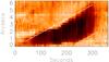 |
Fig. 3 Time-distance plot showing the apparent horizontal velocity of this event. White lines are over-plotted and are used to calculate the gradient of the motion, and hence the velocity within the Hα blue wing. The slit position is shown in Fig. 2. |
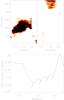 |
Fig. 4 Emission of the Hα line wings for a slit perpendicular to the event, highlighting the small-scale structuring within the events. (Top row) Time-distance plots taken for a slit across the event in the blue wing (left) and red wing (right). We emphasize the threads in this plot by enhancing the contrasts of the image. A black slit is over-plotted to indicate the region plotted with respect to intensity (bottom row). Note, the quadruple intensity minima between 1′′ and 2.5′′ indicated by the arrows. |
To further highlight these smaller structures, difference images were analysed frame-by-frame. We implemented a running difference technique, whereby Diff [x,y,t + 1] = Frame [x,y,t + 1] −Frame [x,y,t], to identify changes in intensity between consecutive frames. In Fig. 5, we plot a representative example of the output of such an analysis, including the image analysed in the bottom frame of Fig. 4, the consecutive frame, and the returned difference image. The white line plotted in the image on the left indicates the slit analysed by Fig. 4. Within the imaging data, it is difficult to see the rapid changes in intensity between the individual fibril events, however, the difference image clearly shows the existence of the small-scale structures. Each of these structures appears to evolve in a similar manner to normal fibrils, showing a marked increase in length (as shown in Fig. 3) and a parabolic shape. Such evolutions have been widely observed within Type I spicules and agree with current theories on p-mode buffeting (de Pontieu et al. 2004) and magnetic reconnection (Yokoyama & Shibata 1996).
 |
Fig. 5 Evolution of the event through time highlighting the fine structured nature of this event. (Left frame) Hα blue wing emission at 17:32:25 UT; the white line indicates the slit selected for analysis in Fig. 4. (Centre frame) Hα blue wing emission at 17:32:27 UT (i.e., the consecutive frame). (Right frame) Difference image between the frames highlighting the fine structures within this event. |
3.3. Links to the photospheric magnetic field
The relationship between surges and strong photospheric magnetic fields has been well documented in recent years (see, for example, Roy 1973a; Madjarska et al. 2009; Kayshap et al. 2013). Often, bright features identified as Ellerman bombs (EBs; first reported by Ellerman 1917) are observed at the footpoints of surges and have been interpreted as evidence of the dynamic nature of the magnetic field co-spatial to the apparent footpoint of these events (for example, Roy 1973b). More recently, links between surges and flux cancellation within an AR have been presented by Chae et al. (1999) and Chen et al. (2009) who suggested that cancellation was evidence supporting reconnection as a driver for the ejection of plasma from the lower chromosphere.
The surge identified in Sects. 3.1 and 3.2 is observed to form co-spatially to a large uni-polar plage region (as is easily seen in the first frame of Fig. 1). The magnetic field within this FOV appears to be stable throughout the course of these data, showing no evidence of flux emergence or cancellation. As has been discussed, the majority of surges analysed by previous researches have found evidence of significant dynamics within co-spatial magnetic fields, however, our results show no such activity. Despite small-scale restructuring of the magnetic field within the plage region being evident co-temporally with the beginning of the absorption feature, it is difficult to quantify how much influence, if any, this has on the ejection.
We, therefore, further analyse the magnetic evolution of this FOV over the course of a two-hour period surrounding the data discussed in this article. This set of data confirms that no bi-polar fields interact to form this event and that only small-scale restructuring occurs within the large uni-polar plage region. This result means that we are unable to present any evidence of magnetic cancellation, or reconnection, leading to the formation of this event. It should be noted that although there are few dynamic changes within the FOV, significant topological complexities of the magnetic field can be inferred through the number and frequency of network bright points, which are often used as a proxy for the vertical magnetic field (see, e.g., Leenaarts et al. 2006). It is, therefore, possible that magnetic structuring on scales smaller than are currently resolvable using the HMI instrument is occuring during this period and leading to reconnection of complex topologies, but the set of data analysed here shows no evidence of this.
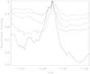 |
Fig. 6 Lightcurves showing the evolution of the upper-atmosphere during the course of this event. Plotted, from bottom to top in the first frame, are the SDO/AIA 304 Å (solid line), 131 Å (long-dashed), 211 Å (dot-dashed), 171 Å (short-dashed), and 193 Å (dot-dot-dot-dashed) filters. |
3.4. Signatures in the transition region and corona
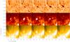 |
Fig. 7 Evolution of the event analysed in this article in the Hα blue wing (top row), SDO/AIA 304 Å (middle row), and 171 Å (bottom row) filters. The difference between each frame is approximately 48 s (starting at 17:28:26 UT and ending at 17:31:37 UT); we estimate that the temporal difference between each wavelength is below 10 s. |
Finally, we assess the effect this event has on the upper atmosphere through an analysis of the SDO/AIA EUV filters. It can be easily inferred from Fig. 1, that a co-spatial brightening event can be seen within the AIA 304 Å and 171 Å filters during a period of strong absorption within the Hα blue wing. Within the 304 Å filter, the peak area of this brightening is approximately 4′′ by 4′′, consistent with the area of a small blinker event (as discussed by, e.g., Chae et al. 2000; Parnell et al. 2002; Madjarska & Doyle 2003). We note, however, that the spatial resolution of the SDO/AIA instrument is significantly higher than the SOHO/CDS instrument used by those researches and, hence, that the scale of this event may appear smaller due to instrumental improvements and not a physical difference.
The evolution of the area of this brightening within the 304 Å filter is roughly parabolic, showing a steady rise to the peak area, before dropping off once again to the background intensity. This parabolic evolution is also apparent within all other SDO/AIA upper atmospheric filters co-temporally, implying that these brightenings are formed as a result of increased density or filling factor in the transition region and corona, rather than a localized heating event, as has been widely suggested in previous researches (see, e.g., Priest et al. 2002). We suggest that the large absorption feature observed within the Hα blue wing is linked to the supply of mass from the lower atmosphere into the upper atmosphere. This presents the open question which is not answered by this article; do smaller fibril structures which are observed within the line wings have a similar, albeit smaller, influence on the upper atmosphere?
The temporal evolution of this event is plotted in Fig. 6 for a number of SDO/AIA filters. A 7′′ by 6′′ box was selected around this apparent small-scale blinker such that no other localized brightening events occurred within the FOV during this period. The average intensity of this box was then calculated for each frame during these observations and plotted for each of five EUV SDO/AIA filters (from bottom to top in the original frame: 304 Å; 131 Å; 211 Å; 171 Å; and 193 Å). The localized brightening event occurs for approximately four minutes which is, once again, the lower boundary for lifetimes of blinkers. The improved cadence of the SDO/AIA instrument over the SOHO/CDS instrument may explain this.
It is interesting to note, that the original brightening in the SDO/AIA filters occurs co-temporally with the initial stages of the formation of the Hα event (similar to the numerical results of Yokoyama & Shibata 1996), before fading entirely whilst there is still strong absorption in the blue wing. In Fig. 7, we plot a visualization of this process. The second frame of Fig. 7 highlights the delay of absorption in the Hα blue wing perfectly. Only the initial stages of development within the Hα blue wing are observed in this frame, but near peak emission in the SDO/AIA 304 Å data are inferred. One possible reason for the time lag within these data could be that we only observe one specific spectral position in each wing within the Hα line and that, therefore, we only receive a snapshot of the whole physical process which is occurring. We note that if full Hα line scan data were available to analyse during this event, a better picture of the observed coupling may have been inferred. We do, however, suggest that this strong absorption feature in the Hα line wing is intrinsically linked to the possible blinker event observed within the SDO/AIA images.
We suggest that the brightening observed within these SDO/AIA data is analogous to a blinker. Although the spatial and temporal scales of this event are on the lower limit of previously observed blinkers (such as those observed by, for example, Harrison 1997; Harrison et al. 1999; Bewsher et al. 2002), the improved spatial and temporal resolutions of the data used within this study may account for this. Combining this result with the large absorption feature within the Hα line wings, interpreted as an on disc surge, presents additional evidence that at least a subset of transient brightening features within the transition region and corona are linked to mass supply from the lower atmosphere. Due to the co-temporal reaction of the Hα line wings and the EUV filters, we suspect that the increased filling factor in the upper atmosphere is caused by a slow shock, propagating away from a reconnection site in the lower atmosphere (in a way described by Yokoyama & Shibata 1996).
4. Discussion
In this article, we have presented a single large-scale absorption feature which is co-temporal to an increased emission from the SDO/AIA transition region and coronal filters. We find strong evidence implying that the absorption feature in the Hα line wings is analogous to jet events, such as surges and macro-spicules, as observed at limb, as well as being linked to the potential small-scale blinker event within the corona.
A question to be addressed is the blinker formation mechanism. Doyle et al. (2004) discussed blinker phenomena being associated with brightenings in pre-existing coronal loops. The brightenings appeared to occur during the emergence of new magnetic flux. These authors suggested that the blinker activity was triggered by interchange reconnection, serving to provide topological connectivity between newly emerging flux and pre-existing flux with the EUV Imaging Telescope (EIT) images showing the existence of loop structures prior to the onset of the blinker activity. The temperature interfaces created in the reconnection process between the cool plasma of the newly emerging loop and the hot plasma of the existing loop was suggested to cause the observed activity seen in both the SUMER and CDS data. As the temperature interfaces propagate with the characteristic speed of a conduction front they heat up the cool chromospheric plasma to coronal temperatures and increase the volume which brightens to transition region temperatures. This was followed-up by Subramanian et al. (2008) who analysed several blinkers and found that in most instances they were associated with the emergence of magnetic flux which gave rise to the appearance of multiple magnetic reconnection events, across an upper atmosphere (coronal) magnetic null point, along with a loop structure as observed with the TRACE 171 Å filter. In a more recent study, Subramanian et al. (2012) classified blinkers into two categories, one associated with coronal counterparts and other with no coronal counterparts as seen in XRT images and EIS 195 Å raster images. Around two-thirds of the blinkers show coronal counterparts and correspond to various events like EUV/X-ray jets, brightenings in coronal bright points or foot-point brightenings of larger loops. The present event fits into those showing a coronal component and matches the slow-shock model presented by Yokoyama & Shibata (1996) suggesting that magnetic reconnection may be the driver of this event.
It should be noted, however, that the lower atmosphere shows no evidence supporting the occurrence of magentic reconnection. Due to the lack of activity within the observed vertical magnetic field, and the structured nature of the absorption event, magnetic reconnection is potentially not the driver of this surge. It is, however, possible that magnetic reconnection is occuring within the lower solar atmosphere, in a manner similar to Ellerman bombs (EBs; see, e.g., Ellerman 1917; Nelson et al. 2013). Both Lee et al. (2003) and Kayshap et al. (2013) found evidence of energy release in the upper solar atmosphere following potential reconnection events in the photosphere. To fully test whether this is the mechanism observed here, we would require a larger statistical sample of surges occuring around uni-polar regions.
Online material
Movie of Fig. 2 Access Supplementary Material
Acknowledgments
Research at the Armagh Observatory is grant-aided by the N. Ireland Dept. of Culture, Arts and Leisure. We thank the National Solar Observatory/Sacramento Peak for their hospitality and in particular Doug Gilliam for his excellent help during the observations. IBIS data reductions were accomplished with help from Kevin Reardon. We thank the UK Science and Technology Facilities Council for CJN’s studentship, PATT T&S support, plus support from STFC grant ST/J001082/1 and the Leverhulme Trust. HMI data are courtesy of SDO (NASA) and the HMI consortium. We would also like to thank Friedrich Wöger for his image reconstruction code.
References
- Berghmans, D., Clette, F., & Moses, D. 1998, A&A, 336, 1039 [NASA ADS] [Google Scholar]
- Bewsher, D., Parnell, C. E., Brown, D. S., & Hood, A. W. 2002, in SOLMAG 2002, Proceedings of the Magnetic Coupling of the Solar Atmosphere Euroconference, ed. H. Sawaya-Lacoste, ESA SP, 505, 239 [Google Scholar]
- Bewsher, D., Parnell, C. E., Pike, C. D., & Harrison, R. A. 2003, Sol. Phys., 215, 217 [NASA ADS] [CrossRef] [Google Scholar]
- Cavallini, F., Berrilli, F., Cantarano, S., & Egidi, A. 2000, in The Solar Cycle and Terrestrial Climate, Solar and Space weather, ed. A. Wilson, ESA SP, 463, 607 [Google Scholar]
- Chae, J., Qiu, J., Wang, H., & Goode, P. R. 1999, ApJ, 513, L75 [NASA ADS] [CrossRef] [Google Scholar]
- Chae, J., Wang, H., Goode, P. R., Fludra, A., & Schühle, U. 2000, ApJ, 528, L119 [NASA ADS] [CrossRef] [PubMed] [Google Scholar]
- Chen, H., Jiang, Y., & Ma, S. 2009, Sol. Phys., 255, 79 [NASA ADS] [CrossRef] [Google Scholar]
- de Pontieu, B., Erdélyi, R., & James, S. P. 2004, Nature, 430, 536 [NASA ADS] [CrossRef] [PubMed] [Google Scholar]
- Doyle, J. G., Roussev, I. I., & Madjarska, M. S. 2004, A&A, 418, L9 [NASA ADS] [CrossRef] [EDP Sciences] [Google Scholar]
- Ellerman, F. 1917, ApJ, 46, 298 [NASA ADS] [CrossRef] [Google Scholar]
- Golub, L. 2006, Space Sci. Rev., 124, 23 [NASA ADS] [CrossRef] [Google Scholar]
- Graham, J. D., Norton, A., López Ariste, A., et al. 2003, in Solar Polarization, eds. J. Trujillo-Bueno, & J. Sanchez Almeida, ASP Conf. Ser., 307, 131 [Google Scholar]
- Harrison, R. A. 1997, Sol. Phys., 175, 467 [NASA ADS] [CrossRef] [Google Scholar]
- Harrison, R. A., Sawyer, E. C., Carter, M. K., et al. 1995, Sol. Phys., 162, 233 [NASA ADS] [CrossRef] [Google Scholar]
- Harrison, R. A., Lang, J., Brooks, D. H., & Innes, D. E. 1999, A&A, 351, 1115 [NASA ADS] [Google Scholar]
- Jiang, Y. C., Chen, H. D., Li, K. J., Shen, Y. D., & Yang, L. H. 2007, A&A, 469, 331 [NASA ADS] [CrossRef] [EDP Sciences] [Google Scholar]
- Kayshap, P., Srivastava, A. K., & Murawski, K. 2013, ApJ, 763, 24 [NASA ADS] [CrossRef] [Google Scholar]
- Lee, J., Gallagher, P. T., Gary, D. E., et al. 2003, ApJ, 585, 524 [NASA ADS] [CrossRef] [Google Scholar]
- Leenaarts, J., Rutten, R. J., Sütterlin, P., Carlsson, M., & Uitenbroek, H. 2006, A&A, 449, 1209 [NASA ADS] [CrossRef] [EDP Sciences] [Google Scholar]
- Lin, Y., Martin, S. F., Engvold, O., Rouppe van der Voort, L. H. M., & van Noort, M. 2008, Adv. Space Res., 42, 803 [NASA ADS] [CrossRef] [Google Scholar]
- Madjarska, M. S., & Doyle, J. G. 2003, A&A, 403, 731 [NASA ADS] [CrossRef] [EDP Sciences] [Google Scholar]
- Madjarska, M. S., Doyle, J. G., Hochedez, J.-F., & Theissen, A. 2006, A&A, 452, L11 [NASA ADS] [CrossRef] [EDP Sciences] [Google Scholar]
- Madjarska, M. S., Doyle, J. G., & de Pontieu, B. 2009, ApJ, 701, 253 [CrossRef] [Google Scholar]
- Nelson, C. J., Doyle, J. G., Erdélyi, R., et al. 2013, Sol. Phys., 283, 307 [NASA ADS] [CrossRef] [Google Scholar]
- O’Shea, E., Banerjee, D., & Doyle, J. G. 2005, A&A, 436, L43 [NASA ADS] [CrossRef] [EDP Sciences] [Google Scholar]
- Parnell, C. E., Bewsher, D., & Harrison, R. A. 2002, Sol. Phys., 206, 249 [NASA ADS] [CrossRef] [Google Scholar]
- Priest, E. R., Hood, A. W., & Bewsher, D. 2002, Sol. Phys., 205, 249 [NASA ADS] [CrossRef] [Google Scholar]
- Roy, J. R. 1973a, Sol. Phys., 32, 139 [NASA ADS] [CrossRef] [Google Scholar]
- Roy, J. R. 1973b, Sol. Phys., 28, 95 [NASA ADS] [CrossRef] [Google Scholar]
- Scherrer, P. H., Bogart, R. S., Bush, R. I., et al. 1995, Sol. Phys., 162, 129 [Google Scholar]
- Subramanian, S., Madjarska, M. S., Maclean, R. C., Doyle, J. G., & Bewsher, D. 2008, A&A, 488, 323 [NASA ADS] [CrossRef] [EDP Sciences] [Google Scholar]
- Subramanian, S., Madjarska, M. S., Doyle, J. G., & Bewsher, D. 2012, A&A, 538, A50 [NASA ADS] [CrossRef] [EDP Sciences] [Google Scholar]
- Teriaca, L., Madjarska, M., & Doyle, J. 2001, Sol. Phys., 200, 91 [NASA ADS] [CrossRef] [Google Scholar]
- Wöger, F., von der Lühe, O., & Reardon, K. 2008, A&A, 488, 375 [NASA ADS] [CrossRef] [EDP Sciences] [Google Scholar]
- Yokoyama, T., & Shibata, K. 1996, PASJ, 48, 353 [NASA ADS] [CrossRef] [Google Scholar]
All Figures
|
Fig. 1 Snapshot of data used in this study at 17:30:01 UT. (Top left) SDO/HMI, (Top right) Hα blue wing, (Bottom left) SDO/AIA 304 Å, and (Bottom right) SDO/AIA 171 Å. The plotted arrow indicates the event which we discuss in this article. |
| In the text | |
|
Fig. 2 Temporal evolution in the blue and red wings of the Hα line profile. (Top row) Evolution of this event through time (from 17:29:42 UT to 17:35:35 UT) in the blue wing (each frame is separated by approximately 70 s). (Bottom row) Corresponding FOV and frames in the red wing showing the apparent parabolic trajectory of this event. The white line indicates an artificial slit used to enable a time-distance plot (shown in Fig. 3). |
| In the text | |
|
Fig. 3 Time-distance plot showing the apparent horizontal velocity of this event. White lines are over-plotted and are used to calculate the gradient of the motion, and hence the velocity within the Hα blue wing. The slit position is shown in Fig. 2. |
| In the text | |
|
Fig. 4 Emission of the Hα line wings for a slit perpendicular to the event, highlighting the small-scale structuring within the events. (Top row) Time-distance plots taken for a slit across the event in the blue wing (left) and red wing (right). We emphasize the threads in this plot by enhancing the contrasts of the image. A black slit is over-plotted to indicate the region plotted with respect to intensity (bottom row). Note, the quadruple intensity minima between 1′′ and 2.5′′ indicated by the arrows. |
| In the text | |
|
Fig. 5 Evolution of the event through time highlighting the fine structured nature of this event. (Left frame) Hα blue wing emission at 17:32:25 UT; the white line indicates the slit selected for analysis in Fig. 4. (Centre frame) Hα blue wing emission at 17:32:27 UT (i.e., the consecutive frame). (Right frame) Difference image between the frames highlighting the fine structures within this event. |
| In the text | |
|
Fig. 6 Lightcurves showing the evolution of the upper-atmosphere during the course of this event. Plotted, from bottom to top in the first frame, are the SDO/AIA 304 Å (solid line), 131 Å (long-dashed), 211 Å (dot-dashed), 171 Å (short-dashed), and 193 Å (dot-dot-dot-dashed) filters. |
| In the text | |
|
Fig. 7 Evolution of the event analysed in this article in the Hα blue wing (top row), SDO/AIA 304 Å (middle row), and 171 Å (bottom row) filters. The difference between each frame is approximately 48 s (starting at 17:28:26 UT and ending at 17:31:37 UT); we estimate that the temporal difference between each wavelength is below 10 s. |
| In the text | |
Current usage metrics show cumulative count of Article Views (full-text article views including HTML views, PDF and ePub downloads, according to the available data) and Abstracts Views on Vision4Press platform.
Data correspond to usage on the plateform after 2015. The current usage metrics is available 48-96 hours after online publication and is updated daily on week days.
Initial download of the metrics may take a while.