© ESO, 2013

1. Introduction

With the recent observations performed with Herschel (e.g. André et al. 2010; Molinari et al. 2010), it has become clearer that filaments are ubiquitous in molecular clouds and that they likely play a central role in star formation. While the exact influence filaments may have on the star formation process remains to be clarified, it is important to understand the properties of these filaments since they are a direct consequence of the physics at play within molecular clouds. In this respect, a particularly intriguing observational result was found by Arzoumanian et al. (2011) who showed that the central widths of the interstellar filaments have a narrow distribution that is peaked around a value of 0.1 pc. Moreover, this characteristic width does not depend on the column density within the filament. Since it is believed that turbulence is important in molecular clouds and largely triggers their evolution, this result is counterintuitive at first sight since turbulence is responsible in a great variety of contexts for producing scale-free power-law distributions. This suggests that there is probably a physical process involved in setting this distribution, which unlike turbulence, presents a characteristic scale.

A recent proposal made by Fischera & Martins (2012, see also Heitsch 2013; Gomez & Vázquez-Semadeni 2013) is that it may result from self-gravitating equilibrium. By solving the hydrostatic equilibrium in an isothermal filament, Fischera & Martins (2012) show that the filament width does not vary significantly and remains on a scale close to the observed 0.1 pc. While this explanation is appealing, a few questions arise. First, it assumes the existence of some confining pressure outside the filament whose nature remains to be specified. Second, it fails to explain why the gravitationally unstable filaments that are collapsing also present this typical width.

In this paper, we explore the idea that the typical width of a self-gravitating filament is due to the combination of accretion-driven turbulence onto the filament, as suggested by the recent velocity dispersion measurements of Arzoumanian et al. (2013), and to the dissipation of this turbulence by ion-neutral friction which does have a characteristic scale. We stress that although ambipolar diffusion is considered here, the underlying idea is totally different from the classical magnetically regulated star formation (e.g. Shu et al. 1987) in which the magnetic field is envisaged as the dominant support and ambipolar diffusion as the process through which the support can be circumvented. In the present picture clouds are typically supercritical. We also note that we do not address the reason why filaments form. As discussed in Hennebelle (2013) this may be due to the shear of the turbulence with a possible further amplification of the anisotropy by gravity for the most massive of them.

The plan of the paper is as follows. In Sect. 2, we present the various assumptions and physical processes used in our simple model. Section 3 describes the results and Sect. 4 concludes the paper.

2. Model and assumptions

2.1. Characteristics of the filament

Herschel observations (e.g. Palmeirim et al. 2013) suggest that the typical average structure of self-gravitating filaments is constituted by i) a central cylinder of nearly uniform density ρ_f and radius r_f; and ii) an envelope whose density profile is ∝r^-2. This radial structure is reminiscent of many self-gravitating objects such as Bonnor-Ebert spheres. More precisely, filaments that are collapsing in a self-similar manner are expected to present an envelope with a profile ∝r^{− 2/(2 − γ)} where γ is the adiabatic index of the gas (Kawachi & Hanawa 1998). As it is likely that self-gravitating filaments are collapsing in a way not too different from, although not identical to, a self-similar collapse, assuming an r^-2 profile is thus a well-motivated assumption, both from observations and theory. One important difference with such self-similar solutions, however, is that the central density plateau does not seem to be shrinking with time.

If L is the length of the filament, the mass of the central part is obviously ${\mathit{M}}_{\mathrm{f}}\mathrm{=}\mathit{\pi }{\mathit{\rho }}_{\mathrm{f}}{\mathit{r}}_{\mathrm{f}}^{\mathrm{2}}\mathit{L}\mathrm{=}{\mathit{m}}_{\mathrm{f}}\mathit{L}$, where M_f is the mass and m_f the mass per unit length. The total mass of the central part plus the surrounding envelope is $\begin{array}{ccc}{\mathit{M}}_{\mathrm{tot}}\mathrm{=}{\mathit{M}}_{\mathrm{f}}\mathrm{[}\mathrm{1}\mathrm{+}\mathrm{2}\ln \mathrm{(}{\mathit{r}}_{\mathrm{ext}}\mathit{/}{\mathit{r}}_{\mathrm{f}}\mathrm{\left)}\mathrm{\right]}\mathrm{\equiv }{\mathit{M}}_{\mathrm{f}}\mathit{\mu }\mathrm{\left(}{\mathit{r}}_{\mathrm{ext}}\mathit{/}{\mathit{r}}_{\mathrm{f}}\mathrm{\right)}\mathit{,}& & \end{array}$(1)where μ(x) = 1 + 2ln(x). It has been assumed that the density outside the filament is ∝1/r² and that the filament stops at some radius r_ext. Below we assume r_ext ≃ L/2.

2.2. Gravitational potential within the filament

The gravitational potential, in the radial direction is obtained by the Gauss’s theorem 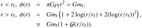$\begin{array}{ccc}\mathit{r}\mathit{<}{\mathit{r}}_{\mathrm{f}}\mathit{,\phi }\mathrm{\left(}\mathit{r}\mathrm{\right)}& \mathrm{=}& \mathit{\pi G}{\mathit{\rho }}_{\mathrm{f}}{\mathit{r}}^{\mathrm{2}}\mathrm{=}\mathit{G}{\mathit{m}}_{\mathrm{f}}\mathit{.}\\ \mathit{r}\mathit{>}{\mathit{r}}_{\mathrm{f}}\mathit{,\phi }\mathrm{\left(}\mathit{r}\mathrm{\right)}& \mathrm{=}& \mathit{G}{\mathit{m}}_{\mathrm{f}}\mathrm{(}\mathrm{1}\mathrm{+}\mathrm{2}\log \mathrm{(}\mathit{r}\mathit{/}{\mathit{r}}_{\mathrm{f}}\mathrm{)}\mathrm{+}\mathrm{2}\mathrm{\left(}\log \mathrm{\right(}\mathit{r}\mathit{/}{\mathit{r}}_{\mathrm{f}}\mathrm{)}{\mathrm{)}}^{\mathrm{2}}\mathrm{)}\mathit{,}\\ & \mathrm{\equiv }& \mathit{G}{\mathit{m}}_{\mathrm{f}}\mathrm{(}\mathrm{1}\mathrm{+}\mathrm{𝒢}\mathrm{(}\mathit{r}\mathit{/}{\mathit{r}}_{\mathrm{f}}\mathrm{\left)}\mathrm{\right)}\mathit{.}\end{array}$(2)where .

2.3. Magnetic field

As the ion-neutral friction dissipation depends on the magnetic field, it is necessary to know its dependence.

We proceed in two steps. First, we discuss the expected value of the magnetic field in the parent clump B_c. Second, we infer the value of the magnetic field in the filament B_f from the value of B_c.

2.3.1. Magnetic field in the parent clump

The magnetic field in the clump is assumed to be proportional to the square root of the density ${\mathit{B}}_{\mathrm{c}}\mathrm{=}{\mathit{B}}_{\mathrm{0}}\sqrt{{\mathit{\rho }}_{\mathrm{c}}\mathit{/}{\mathit{\rho }}_{\mathrm{0}}}$ as has been observed (e.g. Crutcher 1999). Typical values are B₀ ≃ 25  μG and n₀ ≃ 10³ cm^-3, where n₀ = ρ₀/m_p. In the following we will use the ${\mathit{v}}_{\mathrm{A}\mathit{,}\mathrm{0}}\mathrm{=}{\mathit{B}}_{\mathrm{0}}\mathit{/}\sqrt{\mathrm{4}\mathit{\pi }{\mathit{\rho }}_{\mathrm{0}}}\mathrm{\simeq }\mathrm{1}$ km s^-1 as a fiducial value.

We note that the magnetic field dependence is still under debate and that there are alternative choices. First, as suggested by Basu (2000), the magnetic field could scale as $\mathit{\sigma }\sqrt{\mathit{\rho }}$, where σ is the velocity dispersion, rather than just as $\sqrt{\mathit{\rho }}$. Second, Crutcher et al. (2010) now favor B ∝ ρ^2/3. These relations do not represent large variations and would therefore not affect our results very significantly.

2.3.2. Magnetic field in the filament

To link the magnetic field in the filament to the magnetic field in the parent clump, we proceed as follows. First we assume that the magnetic field is perpendicular to the filament. This configuration is well supported by observations in massive filaments such as Taurus (Heyer et al. 2008; Palmeirin et al. 2013) or DR21 (e.g. Kirby 2009), and is also natural on physical grounds as the gas is expected to accumulate preferentially along the field lines. This implies that at least a fraction of the gas accreted by the filament, is not impeded by the magnetic Lorentz force. There may also be gas accreted perpendicularly to the field lines, which is therefore probably slowed down by magnetic pressure. However, if the field is strong, then most of the material is presumably channeled along the field lines, while if the field is weak it also has a weak influence.

Second, we assume flux freezing which at these scales is a reasonable assumption. This implies that the magnetic field in the filament is simply the magnetic field in the clump compressed along the direction perpendicular to the field and the filament axis. Thus B_f ≃ B_c × ηL/r_f since the matter that is inside the radius r_f comes from a distance comparable to the clump’s size, ηL, where η typically varies with time between 0 and 1/2. A similar reasoning can be applied to get a relation between ρ_c and ρ_f since ${\mathit{M}}_{\mathrm{f}}\mathrm{\propto }{\mathit{\rho }}_{\mathrm{f}}{\mathit{r}}_{\mathrm{f}}^{\mathrm{2}}\mathit{L}\mathrm{\simeq }{\mathit{\rho }}_{\mathrm{c}}{\mathit{\eta }}^{\mathrm{2}}{\mathit{L}}^{\mathrm{3}}$. We thus obtain ρ_f = ρ_c(ηL/r_f)². Combining the expression for B_c obtained above with the last expression, we get ${\mathit{B}}_{\mathrm{f}}\mathrm{=}{\mathit{B}}_{\mathrm{0}}\sqrt{\frac{{\mathit{\rho }}_{\mathrm{f}}}{{\mathit{\rho }}_{\mathrm{0}}}}$ that is to say, the magnetic field in the filament is also expected to be nearly proportional to $\sqrt{{\mathit{\rho }}_{\mathrm{f}}}$ implying that the Alfvén velocity should remain nearly constant.

This relation is valid as long as flux freezing can be assumed. While this is a reasonable assumption in the collapsing envelope, which is not magnetically supported, it is not the case in the central part, which is presumably close to equilibrium. The typical ambipolar diffusion timescale is given by Eq. (13) below. For densities on the order of 10^4 − 7 cm^-3, the field is diffused in about 0.1−1 Myr, which is shorter than or comparable to, the accretion time of the filaments. Moreover, as emphasized by Santos-Lima et al. (2012) and Joos et al. (2013), turbulence also tends to diffuse out the field. However since self-gravitating filaments are probably accreting, the magnetic flux cannot leak out far away since it is confined by the infalling gas. Therefore, while the mean magnetic intensity within the central part of these filaments is probably on the order of ${\mathit{B}}_{\mathrm{f}}\mathrm{=}{\mathit{B}}_{\mathrm{0}}\sqrt{\frac{{\mathit{\rho }}_{\mathrm{f}}}{{\mathit{\rho }}_{\mathrm{0}}}}$, it is likely that the magnetic field gradient is greatly reduced with respect to the ideal MHD case.

2.4. Virial equilibrium

The virial theorem is applied to the filament inner part of radius r_f. The expression for a filament is (e.g. Fiege & Pudritz 2000) $\begin{array}{ccc}\mathrm{2}\mathrm{\int }\mathit{P}\mathrm{d}\mathit{V}\mathrm{+}\mathrm{2}{\mathit{E}}_{\mathrm{kin}}^{\mathrm{cyl}}\mathrm{=}{\mathit{W}}_{\mathrm{grav}}\mathrm{+}\mathrm{2}{\mathit{P}}_{\mathrm{ext}}\mathit{V,}& & \end{array}$(3)where W_grav is the gravitational term, P and P_ext are the internal and external pressure, and V the volume; ${\mathit{E}}_{\mathrm{kin}}^{\mathrm{cyl}}\mathrm{=}\mathrm{0.5}{\mathit{M}}_{\mathrm{f}}\mathrm{\left(}\mathrm{2}{\mathit{\sigma }}_{\mathrm{1}\mathrm{D}}^{\mathrm{2}}\mathrm{\right)}$ is the kinetic energy in the direction perpendicular to the filament axis and σ_1D is the non-thermal one-dimensional velocity dispersion. This expression is, however, not strictly valid since our model filament is accreting. Additional terms should be taken into account (see Goldbaum et al. 2011 and Hennebelle 2012) which corresponds to the surface terms that do not cancel out as it is usually the case. When the surface terms are taken into account, the virial expression becomes $\begin{array}{ccc}\frac{\mathrm{1}}{\mathrm{2}}\mathit{Ṁ}\mathrm{2}\frac{\mathrm{d}{\mathit{r}}_{\mathrm{f}}^{\mathrm{2}}}{\mathrm{d}\mathit{M}}\mathrm{+}\mathrm{2}\mathrm{\int }\mathit{P}\mathrm{d}\mathit{V}\mathrm{+}\mathrm{2}{\mathit{E}}_{\mathrm{kin}}^{\mathrm{cyl}}\mathrm{=}{\mathit{W}}_{\mathrm{grav}}\mathrm{+}\mathrm{2}\mathrm{(}{\mathit{P}}_{\mathrm{ext}}\mathrm{+}{\mathit{P}}_{\mathrm{ram}}\mathrm{)}\mathit{V}\mathit{.}& & \end{array}$(4)At this stage we do not consider the influence that the magnetic field may have on the equilibrium because it is not expected to change our conclusions qualitatively. In particular, as discussed in the previous section, the magnetic gradient within the central part of the filament is probably smoothed because of ambipolar diffusion. Another complication arises because the anisotropy introduced by the magnetic field is perpendicular to the filament axis, which would require a bi-dimensional analysis.

Using the different expressions obtained above we get $\begin{array}{ccc}\frac{\mathrm{1}}{\mathrm{2}}\frac{\mathit{ṁ}\begin{array}{c}\mathrm{2}\\ \mathrm{f}\end{array}}{{\mathit{m}}_{\mathrm{f}}}\frac{\mathrm{d}{\mathit{r}}_{\mathrm{f}}^{\mathrm{2}}}{\mathrm{d}{\mathit{m}}_{\mathrm{f}}}\mathrm{+}\mathrm{2}{\mathit{c}}_{\mathrm{s}}^{\mathrm{2}}\mathrm{+}\mathrm{2}{\mathit{\sigma }}_{\mathrm{1}\mathrm{D}}^{\mathrm{2}}\mathrm{=}\mathit{G}{\mathit{m}}_{\mathrm{f}}\mathrm{+}\mathrm{2}\frac{{\mathit{P}}_{\mathrm{ram}}}{{\mathit{\rho }}_{\mathrm{f}}}\mathit{,}& & \end{array}$(5)where P_ram is the ram pressure exerted by the incoming flow and where the pressure of the external medium has not been taken into account. The ram pressure will be estimated below. For the sake of simplicity, we will also use the simplified form of the virial equilibrium $\begin{array}{ccc}\mathrm{2}{\mathit{\sigma }}_{\mathrm{1}\mathrm{D}}^{\mathrm{2}}\mathrm{\simeq }\mathit{G}{\mathit{m}}_{\mathrm{f}}\mathit{.}& & \end{array}$(6)

2.5. Mechanical energy balance

The mechanical energy balance within the cylinder of radius r_f leads to $\begin{array}{ccc}{\mathit{M}}_{\mathrm{f}}\frac{{\mathit{\sigma }}_{\mathrm{3}\mathrm{D}}^{\mathrm{2}}\mathrm{\left(}{\mathit{r}}_{\mathrm{f}}\mathrm{\right)}}{\mathrm{2}{\mathit{\tau }}_{\mathrm{diss}}}\mathrm{\simeq }{\mathit{ϵ}}_{\mathrm{eff}}\mathit{Ṁ}\left(\mathit{\phi }\mathrm{\left(}{\mathit{r}}_{\mathrm{ext}}\mathrm{\right)}\mathrm{-}\mathit{\phi }\mathrm{\left(}{\mathit{r}}_{\mathrm{f}}\mathrm{\right)}\right)\mathit{.}& & \end{array}$(7)Obviously, the left hand-side is the dissipation which can be due either to the turbulence cascade or to the friction between ions and neutrals as described below. We note that it is assumed that the turbulence is isotropic which is why σ_3D is used. The right-hand side describes the source of turbulence which is due to the accretion onto the central part of the filament (Klessen & Hennebelle 2010). The efficiency ϵ_eff is not well known. Klessen & Hennebelle (2010) proposed that it can be related to the density contrast between the density of the incoming flow and the density of the actual gas in which energy is injected. In the present case, the accretion shock may not be clearly defined because of the turbulent nature of the flow. In any case, the present calculation remains largely indicative at this stage. Below, the value ϵ_eff = 0.5 is used because it leads to good agreement with the data. We stress that since our model remains indicative, ϵ_eff could also take into account various other uncertainties. For the sake of simplicity, we have also ignored terms associated to the volume variation and the external pressure (e.g. Goldbaum et al. 2011) as they do not modify the results substantially, but make the mechanical energy balance much more complex.

2.6. Accretion rate

The accretion rate remains uncertain since it is difficult to infer observationally (see however Palmeirim et al. 2013 for an estimate in the case of the Taurus B211/3 filament). Here, we consider two different possibilities. This will allow us to test the robustness of our conclusion.

2.6.1. Gravitational accretion rate

To estimate the accretion rate, we assume that it can be computed from the density within the parent clump and the infall velocity. Assuming that the parent clump has a cylindrical radius of about L/2 and a length equal to L, we get Ṁ = πL²ρ_cV_inf.

The infall velocity is due to the gravitational field of the filament which is given by Eq. (2). We assume that the material which enters the clump at radius r ≃ L/2 has no initial velocity and we estimate the infall velocity at r = L/4 leading for V_inf to $\begin{array}{ccc}{\mathit{V}}_{\inf }\mathrm{\simeq }\sqrt{\mathrm{2}\mathit{G}{\mathit{m}}_{\mathrm{f}}}{\left(\mathrm{𝒢}\left(\frac{\mathit{L}}{\mathrm{2}{\mathit{r}}_{\mathrm{f}}}\right)\mathrm{-}\mathrm{𝒢}\left(\frac{\mathit{L}}{\mathrm{4}{\mathit{r}}_{\mathrm{f}}}\right)\right)}^{\mathrm{1}\mathit{/}\mathrm{2}}\mathrm{·}& & \end{array}$(8)We note that this is again a rough estimate, but since the gravitational potential varies logarithmically with r, this estimate does not depend severely on these assumptions.

The density within the clump is also needed to get the accretion rate and we assume that ρ_c = m_pn_c follows the Larson relations (Larson 1981; Falgarone et al. 2009; Hennebelle & Falgarone 2012), m_p being the mass per particle 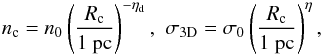$\begin{array}{ccc}{\mathit{n}}_{\mathrm{c}}\mathrm{=}{\mathit{n}}_{\mathrm{0}}{\left(\frac{{\mathit{R}}_{\mathrm{c}}}{\mathrm{1}\mathrm{pc}}\right)}^{\mathrm{-}{\mathit{\eta }}_{\mathrm{d}}}\mathit{,}\hspace{0.17em}\hspace{0.17em}{\mathit{\sigma }}_{\mathrm{3}\mathrm{D}}\mathrm{=}{\mathit{\sigma }}_{\mathrm{0}}{\left(\frac{{\mathit{R}}_{\mathrm{c}}}{\mathrm{1}\mathrm{pc}}\right)}^{\mathit{\eta }}\mathit{,}& & \end{array}$(9)where n_c is the clump gas density and σ_3D the internal rms velocity. The exact values of the various coefficients remain somewhat uncertain. Originally, Larson (1981) estimated η_d ≃ 1.1 and η ≃ 0.38, but more recent estimates (Falgarone et al. 2009) using larger sets of data suggest that η_d ≃ 0.7 and η ≃ 0.45 − 0.5. For the sake of simplicity, we use η_d = 1 and take n₀ = 1000 cm^-3. 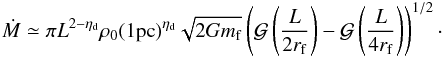$\begin{array}{ccc}\mathit{Ṁ}\mathrm{\simeq }\mathit{\pi }{\mathit{L}}^{\mathrm{2}\mathrm{-}{\mathit{\eta }}_{\mathrm{d}}}{\mathit{\rho }}_{\mathrm{0}}\mathrm{(}\mathrm{1}\mathrm{pc}{\mathrm{)}}^{{\mathit{\eta }}_{\mathrm{d}}}\sqrt{\mathrm{2}\mathit{G}{\mathit{m}}_{\mathrm{f}}}{\left(\mathrm{𝒢}\left(\frac{\mathit{L}}{\mathrm{2}{\mathit{r}}_{\mathrm{f}}}\right)\mathrm{-}\mathrm{𝒢}\left(\frac{\mathit{L}}{\mathrm{4}{\mathit{r}}_{\mathrm{f}}}\right)\right)}^{\mathrm{1}\mathit{/}\mathrm{2}}\mathrm{·}& & \end{array}$(10)The typical accretion timescale is simply given by τ_accret = M/Ṁ. With Eq. (10), it is easy to show that ${\mathit{\tau }}_{\mathrm{accret}}\mathrm{\propto }\sqrt{{\mathit{\rho }}_{\mathrm{f}}}$.

2.6.2. Turbulent accretion rate

As it is not clear what controls the accretion rates onto interstellar filaments, we also consider the turbulent accretion rate constructed from the Larson relations described in Hennebelle (2012), 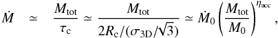$\begin{array}{ccc}\mathit{Ṁ}& \mathrm{\simeq }& \frac{{\mathit{M}}_{\mathrm{tot}}}{{\mathit{\tau }}_{\mathrm{c}}}\mathrm{\simeq }\frac{{\mathit{M}}_{\mathrm{tot}}}{\mathrm{2}{\mathit{R}}_{\mathrm{c}}\mathit{/}\mathrm{(}{\mathit{\sigma }}_{\mathrm{3}\mathrm{D}}\mathit{/}\sqrt{\mathrm{3}}\mathrm{)}}\mathrm{\simeq }\mathit{Ṁ}\mathrm{0}{\left(\frac{{\mathit{M}}_{\mathrm{tot}}}{{\mathit{M}}_{\mathrm{0}}}\right)}^{{\mathit{\eta }}_{\mathrm{acc}}}\mathit{,}\end{array}$(11)where η_acc ≃ 0.7 − 0.8 depending on the exact choice of the parameter η and η_d that is retained. We will adopt η_acc ≃ 0.75 as a fiducial value. We typically have Ṁ₀ = 10^-3  M_⊙ yr^-1 for M₀ = 10⁴  M_⊙.

2.6.3. Ram pressure

The ram pressure which appears in Eq. (5) can be estimated as follows. It is equal to the product of V_inf(r_f)² and ρ_in = Ṁ/(2πr_fLV_inf(r_f)), where ρ_in is the density that is obtained assuming a constant accretion rate. We note that ρ_in < ρ_f, which implies that an accretion shock is connecting the infalling envelope and the central part of the filament. Since the above expression assumes that the flow is isotropic, and since we are assuming the structure of the flow rather than inferring an exact solution, this value remains hampered by large uncertainties and is certainly valid within a factor of a few. We have tested the influence of vaying the ram pressure by a factor of a few and found that it has a limited influence on the solution at low density, while it has no influence at high density.

2.7. Dissipation timescales

The dissipation timescale to be used in Eq. (7) is a crucial issue. Here we emphasize two dissipation mechanisms, the turbulent cascade time and the ambipolar diffusion time. Quantitative estimates of these two timescales have been recently estimated by Li et al. (2012) in turbulent two fluid MHD simulations. They found that under typical molecular cloud conditions both contribute, but the second dominates over the first.

2.7.1. Dissipation by turbulent cascade

First, we consider the standard turbulent cascade timescale, which is the crossing time of the system 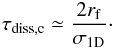$\begin{array}{ccc}{\mathit{\tau }}_{\mathrm{diss}\mathit{,}\mathrm{c}}\mathrm{\simeq }\frac{\mathrm{2}{\mathit{r}}_{\mathrm{f}}}{{\mathit{\sigma }}_{\mathrm{1}\mathrm{D}}}\mathrm{·}& & \end{array}$(12)The energy cascades to smaller and smaller scales until the size of the eddies reaches the viscous scale.

2.7.2. Dissipation by ion-neutral friction

Second, we investigate the dissipation induced by the ion-neutral friction. Its expression was first inferred by Kulsrud & Pearce (1969, see also Lequeux 2005) and is given by $\begin{array}{ccc}{\mathit{\tau }}_{\mathrm{diss}\mathit{,}\mathrm{amb}}\mathrm{=}\frac{\mathrm{2}{\mathit{\gamma }}_{\mathrm{damp}}{\mathit{\rho }}_{\mathit{i}}}{{\mathit{v}}_{\mathrm{A}}^{\mathrm{2}}\mathrm{(}\mathrm{2}\mathit{\pi }\mathit{/}\mathit{\lambda }{\mathrm{)}}^{\mathrm{2}}}\mathrm{=}\frac{\mathrm{2}{\mathit{\nu }}_{\mathrm{ni}}}{{\mathit{v}}_{\mathrm{A}}^{\mathrm{2}}\mathrm{(}\mathrm{2}\mathit{\pi }\mathit{/}\mathit{\lambda }{\mathrm{)}}^{\mathrm{2}}}\mathit{,}& & \end{array}$(13)where v_A is the Alfvén speed, λ is the wavelength assumed to be equal to r_f and ν_ni is the ion-neutral coupling coefficient. The reason we choose λ ≃ r_f is that if most of the energy is dissipated at a scale much smaller than r_f, then the relevant time would be the crossing or cascading time that would be necessary for the energy to cascade from r_f. In this case, the timescale would thus be similar to the turbulent cascade timescale discussed above. The coefficient γ_damp = 3.5 × 10¹³ cm³ g^-1 s^-1 is the damping rate. The ion density, ρ_i is assumed to be ${\mathit{\rho }}_{\mathit{i}}\mathrm{=}\mathit{C}\sqrt{{\mathit{\rho }}_{\mathit{n}}}$ where C = 3 × 10^-16 cm^−3/2 g^1/2. For wavelengths λ < λ_c = πv_A/(γ_dampρ_i), the critical wavelength, the Alfvén waves do not even propagate except at very small wavelengths when the ions and the neutrals are entirely decoupled. With n ≃ 10⁴ cm^-3 and v_A ≃ 1 km s^-1, λ_c ≃ 5 × 10^-2 pc.

We note that the expression stated in Eq. (13) is strictly valid only for Alfvén waves. The corresponding expression for the compressible modes has been inferred by Ferrière et al. (1988). They are slightly more complex as it entails the angle between the field and the direction of propagation, but the order of magnitude is not different.

3. Results

To infer the radius of the filament as a function of the central density ρ_f we have to combine Eqs. (2), (6), and (7) together with the accretion rate given by Eq. (10) or Eq. (11). With the gravitational accretion rate (Eq. (10)), we obtain $\begin{array}{ccc}\frac{{\mathit{\rho }}_{\mathrm{f}}^{\mathrm{1}\mathit{/}\mathrm{2}}{\mathit{r}}_{\mathrm{f}}}{{\mathit{\tau }}_{\mathrm{diss}}}\mathrm{=}\frac{\mathrm{4}}{\mathrm{3}}\sqrt{\mathrm{2}\mathit{\pi }}{\mathit{ϵ}}_{\mathrm{eff}}{\mathit{\rho }}_{\mathrm{0}}\mathrm{\left(}\mathrm{1}\mathrm{pc}\mathrm{\right)}\sqrt{\mathit{G}}{\mathrm{𝒢}}_{\mathrm{1}}\mathrm{(}\mathit{L}\mathit{/}{\mathit{r}}_{\mathrm{f}}\mathrm{)}\mathit{,}& & \end{array}$(14)where . With the turbulent accretion rate (Eq. (11)), we get the relation $\begin{array}{ccc}\frac{\mathrm{(}\mathit{\pi }{\mathit{\rho }}_{\mathrm{f}}{\mathit{r}}_{\mathrm{f}}^{\mathrm{3}}{\mathrm{)}}^{\mathrm{1}\mathrm{-}{\mathit{\eta }}_{\mathrm{acc}}}}{{\mathit{\tau }}_{\mathrm{diss}}}\mathrm{=}\frac{\mathrm{4}{\mathit{ϵ}}_{\mathrm{eff}}\mathit{Ṁ}\mathrm{0}{\mathrm{𝒢}}_{\mathrm{2}}\mathrm{(}\mathit{L}\mathit{/}{\mathit{r}}_{\mathrm{f}}\mathrm{)}}{\mathrm{3}{\mathit{M}}_{\mathrm{0}}^{{\mathit{\eta }}_{\mathrm{acc}}}\mathrm{(}\mathit{L}\mathit{/}{\mathit{r}}_{\mathrm{f}}{\mathrm{)}}^{\mathrm{1}\mathrm{-}{\mathit{\eta }}_{\mathrm{acc}}}}& & \end{array}$(15)where .

3.1. Dynamical equilibrium with turbulent dissipation

Combining Eq. (12) with Eq. (6), we get ${\mathit{\tau }}_{\mathrm{diss}}\mathrm{=}\frac{\mathrm{2}\sqrt{\mathrm{2}}}{\sqrt{\mathit{\pi G}{\mathit{\rho }}_{\mathrm{f}}}}$ which in turn together with Eq. (15) leads to the expression $\begin{array}{ccc}{\mathit{r}}_{\mathrm{f}}\mathrm{=}{\mathit{\rho }}_{\mathrm{f}}^{\frac{{\mathit{\eta }}_{\mathrm{acc}}\mathrm{-}\mathrm{3}\mathit{/}\mathrm{2}}{\mathrm{3}\mathrm{(}\mathrm{1}\mathrm{-}{\mathit{\eta }}_{\mathrm{acc}}\mathrm{)}}}{\left(\frac{\mathrm{8}\sqrt{\mathrm{2}}}{\mathrm{3}{\mathit{\pi }}^{\mathrm{3}\mathit{/}\mathrm{2}\mathrm{-}{\mathit{\eta }}_{\mathrm{acc}}}\sqrt{\mathit{G}}}\frac{{\mathit{ϵ}}_{\mathrm{eff}}\mathit{Ṁ}\mathrm{0}{\mathrm{𝒢}}_{\mathrm{2}}\mathrm{(}\mathit{L}\mathit{/}{\mathit{r}}_{\mathrm{f}}\mathrm{)}}{{\mathit{M}}_{\mathrm{0}}^{{\mathit{\eta }}_{\mathrm{acc}}}\mathrm{(}\mathit{L}\mathit{/}{\mathit{r}}_{\mathrm{f}}{\mathrm{)}}^{\mathrm{1}\mathrm{-}{\mathit{\eta }}_{\mathrm{acc}}}}\right)}^{\frac{\mathrm{1}}{\mathrm{3}\mathrm{(}\mathrm{1}\mathrm{-}{\mathit{\eta }}_{\mathrm{acc}}\mathrm{)}}}\mathrm{·}& & \end{array}$(16)For the canonical value η_acc = 0.75, we find that r_f ∝ 1/ρ_f. That is to say, the typical filament radius decreases with the central density as displayed in Fig. 1 (see the line labeled turbulence). The value ϵ_eff = 0.5 has been used in this calculation. For larger values of η_acc we still get significant variations of r_f with ρ_f. For η_acc = 1 we would even predict that the central density is independent of r_f. A filament radius independent of the central density is obtained only for η_acc ≃ 3/2. The gravitational accretion rate expression leads to a very similar expression with r_f ∝ 1/ρ_f and the corresponding expression is not given here for conciseness as the obvious conclusion is that this behaviour is incompatible with a nearly constant filament width.

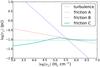Fig. 1 Filament radius as a function of filament density for four models. The curve labeled turbulence shows the result for a turbulent crossing time (Eq. (16)); the three curves labeled friction show results when ion-neutral friction time is assumed to be the energy dissipation time (Eqs. (17)−(18)). Frictions A and C used a gravitational accretion rate and Friction B a turbulent rate.

3.2. Dynamical equilibirum with ion-neutral friction

Combining Eqs. (13) and (6), with (14), we infer $\begin{array}{ccc}{\mathit{r}}_{\mathrm{f}}\mathrm{=}\frac{\mathrm{3}{\mathit{\pi }}^{\mathrm{3}\mathit{/}\mathrm{2}}{\mathit{v}}_{\mathrm{a}\mathit{,}\mathrm{0}}^{\mathrm{2}}}{\mathrm{2}\sqrt{\mathrm{2}}{\mathit{ϵ}}_{\mathrm{eff}}{\mathit{\gamma }}_{\mathrm{damp}}\mathit{C}{\mathit{\rho }}_{\mathrm{0}}\mathrm{\left(}\mathrm{1}\mathrm{pc}\mathrm{\right)}\sqrt{\mathit{G}}{\mathrm{𝒢}}_{\mathrm{1}}\mathrm{(}\mathit{L}\mathit{/}{\mathit{r}}_{\mathrm{f}}\mathrm{)}}\mathit{,}& & \end{array}$(17)where we see that r_f does not depend on ρ_f. That is to say, the width of the filament does not change with its column density as suggested from the results of Arzoumanian et al. (2011). To test the robustness of this result, it is worth investigating what the turbulent accretion rate stated by Eq. (11) is predicting. The corresponding expression is $\begin{array}{ccc}{\mathit{r}}_{\mathrm{f}}\mathrm{=}{\mathit{\rho }}_{\mathrm{f}}^{\frac{{\mathit{\eta }}_{\mathrm{acc}}\mathrm{-}\mathrm{1}\mathit{/}\mathrm{2}}{\mathrm{1}\mathrm{-}\mathrm{3}{\mathit{\eta }}_{\mathrm{acc}}}}{\left(\frac{\mathrm{2}{\mathit{\gamma }}_{\mathrm{damp}}\mathit{C}}{\mathrm{3}{\mathit{\pi }}^{\mathrm{3}\mathrm{-}{\mathit{\eta }}_{\mathrm{acc}}}{\mathit{v}}_{\mathrm{a}\mathit{,}\mathrm{0}}^{\mathrm{2}}}\frac{{\mathit{ϵ}}_{\mathrm{eff}}\mathit{Ṁ}\mathrm{0}{\mathrm{𝒢}}_{\mathrm{2}}\mathrm{(}\mathit{L}\mathit{/}{\mathit{r}}_{\mathrm{f}}\mathrm{)}}{{\mathit{M}}_{\mathrm{0}}^{{\mathit{\eta }}_{\mathrm{acc}}}\mathrm{(}\mathit{L}\mathit{/}{\mathit{r}}_{\mathrm{f}}{\mathrm{)}}^{\mathrm{1}\mathrm{-}{\mathit{\eta }}_{\mathrm{acc}}}}\right)}^{\frac{\mathrm{1}}{\mathrm{1}\mathrm{-}\mathrm{3}{\mathit{\eta }}_{\mathrm{acc}}}}\mathrm{·}& & \end{array}$(18)As can be seen for an accretion rate exponent η_acc of the order of 0.75, we find that ${\mathit{r}}_{\mathrm{f}}\mathrm{\propto }{\mathit{\rho }}_{\mathrm{f}}^{-0.2}$, which implies a very weak dependence on the filament radius r_f. For a value of η_acc = 1, we have ${\mathit{r}}_{\mathrm{f}}\mathrm{\propto }{\mathit{\rho }}_{\mathrm{f}}^{\mathrm{-}\mathrm{1}\mathit{/}\mathrm{4}}$ which is still a shallow dependence as shown in Fig. 1 where the two expressions stated by Eqs. (17) and (18) are displayed (labeled as friction A and B, respectively).

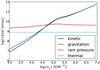Fig. 2 Amplitude of the various terms which appear in the virial equilibrium (Eq. (5)). While at high density the filament equilibrium is due to the balance between gravity and velocity dispersion, it is due to the balance between ram and thermal pressure at low density.

3.3. A more accurate model

Finally, we investigate the solutions where the thermal support and ram pressure are considered as stated in Eq. (5). The corresponding curve is labeled as friction C. Equation (5) is an ordinary differential equation in r_f, which can be solved using a standard Runge-Kutta method. Since it is necessary to specify a radius and a density to start the integration, we have explored various cases. We found that for a large range of radii (r_start ≃ 0.01 − 0.1 pc) at low density, the solutions quickly converge towards the one that is presented here and for which the radius at n = 10³ cm^-3 is equal to about 0.05 pc.

As can be seen, more variability is introduced, particularly at low density, where we see that the filament radius decreases at low density. In order to better understand the physical meaning of this solution we plot in Fig. 2, the values of the various virial terms as a function of density.

While the equilibrium between gravity and turbulent support at high density is robust and independent of the choice of the boundary condition, r_start, the behaviour at low density is less robust and varies with it.

It is important to stress a few points. First, the ram pressure term which causes most of the variation remains uncertain since our model is not fully self-consistent in the sense that the density and velocity fields, although reasonable, are not proper solutions of the problem. Second, in the low density regime, the filament is not gravitationally accreting and it is likely that the validity of the model is questionable.

3.4. Comparison of the two dissipation timescales

It is enlighting to compare the values of the dissipation timescales as a function of density for the filament radius corresponding to model B. As expected, the turbulent dissipation timescale is much longer than the ion-neutral friction timescale for densities lower than 10⁶ cm^-3. It also increases with density while the turbulent timescale decreases with density. This behaviour is the very reason which explains the nearly constant width of the filaments in our model because as can be seen in Fig. 3, the accretion time presents the same dependence.

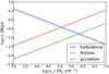Fig. 3 Comparison between the turbulent dissipation and ion-neutral friction times as a function of density. Also shown is the accretion timescale. It scales exactly as the ion-neutral friction time does.

To summarize, assuming that the relevant timescale for energy dissipation within the central part of the filament is the turbulent crossing time, we find under reasonable assumptions for the accretion rate that the width changes significantly with density. This is because τ_diss,c ∝ 1/$\sqrt{{\mathit{\rho }}_{\mathrm{f}}}$. On the other hand, when we assume that the relevant timescale for energy dissipation is the ion-neutral friction time, we find that the width varies much less with the filament density. This is because, ${\mathit{\tau }}_{\mathrm{diss}\mathit{,}\mathrm{amb}}\mathrm{\propto }{\mathit{\rho }}_{\mathit{i}}\mathrm{\propto }\sqrt{{\mathit{\rho }}_{\mathrm{f}}}\mathrm{\propto }{\mathit{\tau }}_{\mathrm{accret}}$. Since the relevant timescale is the shortest one, which corresponds to the smallest value of r_f, one expects ion-neutral friction to be the dominant mechanism for energy dissipation up to densities of a few 10⁵ − 10⁶ cm^-3 (see Fig. 1).

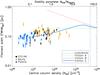Fig. 4 Comparison between the models and the filaments width distribution (adapted from Arzoumanian et al. 2011).

3.5. Comparison with observations

Finally, we confront the present models with the Herschel observational result of Arzoumanian et al. (2011). Figure 4 shows filament width as a function of filament column density. As can be seen, the model based on ion-neutral friction and gravitational accretion (friction B and C) work very well. We note that the model based on turbulent dissipation predicts a constant column density and a variable radius.

4. Conclusion

We have presented a simple model to describe the evolution of accreting self-gravitating filaments within molecular clouds. It assumes virial equilibrium between gravity and turbulence and mechanical energy balance between accretion which drives turbulence in the filament and the dissipation of this energy. We show that while dissipation based on turbulent cascade fails to reproduce the narrow range of radius inferred from Herschel observations, dissipation based on ion-neutral friction leads to a filament width that depends only weakly on the filament density and is very close to the ≃0.1 pc value, although our analytical approach is hampered by significant uncertainties. We conclude that the combination of accretion-driven turbulence and ion-neutral friction is a promising mechanism to explain the structure of self-gravitating filaments and deserves further investigation.

Acknowledgments

We thank the anonymous referee for a constructive and helpful report. We thank Doris Arzoumanian and Evangelia Ntormousi for discussions on this topic. P.H. acknowledge the financial support of the Agence National pour la Recherche through the COSMIS project. This research has received funding from the European Research Council under the European Community’s Seventh Framework Programme (FP7/2007−2013 Grant Agreements No. 306483 and No. 291294).

References

All Figures

	Fig. 1 Filament radius as a function of filament density for four models. The curve labeled turbulence shows the result for a turbulent crossing time (Eq. (16)); the three curves labeled friction show results when ion-neutral friction time is assumed to be the energy dissipation time (Eqs. (17)−(18)). Frictions A and C used a gravitational accretion rate and Friction B a turbulent rate.
In the text

	Fig. 2 Amplitude of the various terms which appear in the virial equilibrium (Eq. (5)). While at high density the filament equilibrium is due to the balance between gravity and velocity dispersion, it is due to the balance between ram and thermal pressure at low density.
In the text

	Fig. 3 Comparison between the turbulent dissipation and ion-neutral friction times as a function of density. Also shown is the accretion timescale. It scales exactly as the ion-neutral friction time does.
In the text

	Fig. 4 Comparison between the models and the filaments width distribution (adapted from Arzoumanian et al. 2011).
In the text

References

- André, P., Men’shchikov, A., Bontemps, S., et al. 2010, A&A, 518, L102 [NASA ADS] [CrossRef] [EDP Sciences] [Google Scholar]
- Arzoumanian, D., André, Ph., Didelon, P., et al. 2011, A&A, 529, L6 [Google Scholar]
- Arzoumanian, D., André, Ph., Peretto, N., & Konyves, V. 2013, A&A, 553, A119 [NASA ADS] [CrossRef] [EDP Sciences] [Google Scholar]
- Basu, S. 2000, ApJ, 540, L103 [NASA ADS] [CrossRef] [Google Scholar]
- Crutcher, R. 1999, ApJ, 520, 706 [NASA ADS] [CrossRef] [Google Scholar]
- Crutcher, R., Wandelt, B., Heiles, C., Falgarone, E., & Troland, T. 2010, ApJ, 725, 466 [NASA ADS] [CrossRef] [Google Scholar]
- Falgarone, E., Pety, J., & Hily-Blant, P. 2009, A&A, 507, 355 [NASA ADS] [CrossRef] [EDP Sciences] [Google Scholar]
- Ferrière, K., Zweibel, E., & Shull, J. 1988, ApJ, 332, 984 [NASA ADS] [CrossRef] [Google Scholar]
- Fiege, J., & Pudritz, R. 2000, MNRAS, 311, 85 [NASA ADS] [CrossRef] [Google Scholar]
- Fischera, J., & Martin, P. 2012, A&A, 542, A77 [NASA ADS] [CrossRef] [EDP Sciences] [Google Scholar]
- Goldbaum, N., Krumholz, M., Matzner, C., & McKee, C. 2011, ApJ, 738, 101 [NASA ADS] [CrossRef] [Google Scholar]
- Gomez, G., & Vàquez-Semadeni, E. 2013, ApJ, submitted [arXiv:1308.6298] [Google Scholar]
- Heitsch, F. 2013, ApJ, 769, 115 [NASA ADS] [CrossRef] [Google Scholar]
- Hennebelle, P. 2012, A&A, 545, A147 [NASA ADS] [CrossRef] [EDP Sciences] [Google Scholar]
- Hennebelle, P. 2013, A&A, 556, A153 [NASA ADS] [CrossRef] [EDP Sciences] [Google Scholar]
- Hennebelle, P., & Falgarone, E. 2012, A&ARv, 20, 55 [NASA ADS] [CrossRef] [Google Scholar]
- Heyer, M., Gong, H., Ostriker, E., & Brunt, C. 2008, ApJ, 680, 420 [NASA ADS] [CrossRef] [Google Scholar]
- Joos, M., Hennebelle, P., Ciardi, A., & Fromang, S. 2013, A&A, 554, A17 [NASA ADS] [CrossRef] [EDP Sciences] [Google Scholar]
- Kawachi, T., & Hanawa, T. 1998, PASP, 50, 577 [Google Scholar]
- Kirby, L. 2009, ApJ, 694, 1056 [NASA ADS] [CrossRef] [Google Scholar]
- Klessen, R., & Hennebelle, P. 2010, A&A, 520, A17 [NASA ADS] [CrossRef] [EDP Sciences] [Google Scholar]
- Kulsrud, R., & Pearce, W. 1969, ApJ, 156, 445 [Google Scholar]
- Larson, R. 1981, MNRAS, 194, 809 [CrossRef] [Google Scholar]
- Lequeux, J. 2005, The interstellar medium (Springer) [Google Scholar]
- Li, P.-S., Myers, A., & McKee, C. 2012, ApJ, 760, 33 [NASA ADS] [CrossRef] [Google Scholar]
- Molinari, S., Swinyard, B., & Bally, J. 2010, A&A, 518, L100 [NASA ADS] [CrossRef] [EDP Sciences] [Google Scholar]
- Palmeirim, P., André, Ph., Kirk, J., et al. 2013, A&A, 550, A38 [NASA ADS] [CrossRef] [EDP Sciences] [Google Scholar]
- Santos-Lima, R., de Gouveia Dal Pino, E., & Lazarian, A. 2012, ApJ, 747, 21 [NASA ADS] [CrossRef] [Google Scholar]
- Shu, F. H., Adams, F. C., & Lizano, S. 1987, ARA&A, 25, 23 [Google Scholar]