| Issue |
A&A
Volume 560, December 2013
|
|
|---|---|---|
| Article Number | A86 | |
| Number of page(s) | 11 | |
| Section | Cosmology (including clusters of galaxies) | |
| DOI | https://doi.org/10.1051/0004-6361/201321618 | |
| Published online | 10 December 2013 | |
Analytic solutions for Navarro-Frenk-White lens models in the strong lensing regime for low characteristic convergences
Instituto de Cosmologia, Relatividade e Astrofísica – ICRA, Centro Brasileiro de Pesquisas Físicas, rua Dr. Xavier Sigaud 150, CEP 22290-180, Rio de Janeiro RJ, Brazil
e-mail: This email address is being protected from spambots. You need JavaScript enabled to view it.
Received: 1 April 2013
Accepted: 23 September 2013
Abstract
Context. The Navarro-Frenk-White (NFW) density profile is often used to model gravitational lenses. For κs ≲ 0.1 (where κs is a parameter that defines the normalization of the NFW lens potential) – corresponding to galaxy and galaxy group mass scales – high numerical precision is required to accurately compute several quantities in the strong lensing regime.
Aims. We obtain analytic solutions for several lensing quantities for circular NFW models and their elliptical (ENFW) and pseudo-elliptical (PNFW) extensions, on the typical scales where gravitational arcs are expected to be formed, in the κs ≲ 0.1 limit, by establishing their domain of validity.
Methods. We approximate the deflection angle of the circular NFW model and derive analytic expressions for the convergence and shear for the PNFW and ENFW models. We obtain the constant distortion curves (including the tangential critical curve), which are used to define the domain of validity of the approximations, by employing a figure-of-merit to compare with the exact numerical solutions. We compute the deformation cross section as a further check of the validity of the approximations.
Results. We derive analytic solutions for iso-convergence contours and constant distortion curves for the models considered here. We also obtain the deformation cross section, which is given in closed form for the circular NFW model and in terms of a one-dimensional integral for the elliptical ones. In addition, we provide a simple expression for the ellipticity of the iso-convergence contours of the pseudo-elliptical models and the connection of characteristic convergences among the PNFW and ENFW models.
Conclusions. We conclude that the set of solutions derived here is generally accurate for κs ≲ 0.1. For low ellipticities, values up to κs ≃ 0.18 are allowed. On the other hand, the mapping among PNFW and the ENFW models is valid up to κs ≃ 0.4. The solutions derived in this work can be used to speed up numerical codes and ensure their accuracy in the low κs regime, including applications to arc statistics and other strong lensing observables.
Key words: gravitational lensing: strong / galaxies: halos / galaxies: groups: general / dark matter
© ESO, 2013
1. Introduction
Gravitational arcs are powerful tools to probe the mass distribution in galaxies (Koopmans et al. 2009; Barnabè et al. 2011; Suyu et al. 2012) and clusters of galaxies (Kovner 1989; Miralda-Escude 1993; Hattori et al. 1997; Comerford et al. 2006). In addition, their abundance can help to constrain cosmological models (Bartelmann et al. 1998; Golse et al. 2002; Bartelmann et al. 2003; Meneghetti et al. 2005; Jullo et al. 2010).
Two techniques have been used to extract information from gravitational arcs. The first is arc-statistics: counting arcs as a function of their properties, such as the length-to-width ratio or angular separation, for a lens sample (Wu & Hammer 1993; Grossman & Saha 1994; Bartelmann & Weiss 1994; Bartelmann et al. 1995; Bartelmann 1995). The second is inverse modeling: using arcs in individual clusters or galaxies aiming to determine the mass distribution of the lens and source properties (Kneib et al. 1993; Keeton 2001b; Golse et al. 2002; Wayth & Webster 2006; Jullo et al. 2007, 2010).
These approaches have motivated arc searches in wide field surveys (Gladders et al. 2003; Estrada et al. 2007; Cabanac et al. 2007; Belokurov et al. 2009; Kubo et al. 2010; Kneib et al. 2010; Gilbank et al. 2011; Wen et al. 2011; More et al. 2012; Bayliss 2012; Wiesner et al. 2012, Erben et al., in prep.), as well as in images targeting clusters (Luppino et al. 1999; Ebeling et al. 2001; Zaritsky & Gonzalez 2003; Smith et al. 2005; Sand et al. 2005; Hennawi et al. 2008; Kausch et al. 2010; Horesh et al. 2011; Furlanetto et al. 2013; Postman et al. 2012) and galaxies (Ratnatunga et al. 1999; Fassnacht et al. 2004; Bolton et al. 2006; Willis et al. 2006; Moustakas et al. 2007; Kubo & Dell’Antonio 2008; Faure et al. 2008; Jackson 2008). Moreover, the upcoming wide-field surveys, such as the Dark Energy Survey1 (Annis et al. 2005, Frieman et al., in prep.; Lahav et al., in prep.), which started taking data in 2012, are expected to detect strong lensing systems in the thousands, about an order of magnitude more than the current homogeneous samples.
A widely used model for representing the radial distribution of dark matter from galaxy to cluster of galaxies mass scales is the Navarro-Frenk-White profile (Navarro et al. 1996, 1997, hereafter NFW), whose mass density is given by  (1)where rs and ρs are the scale radius and characteristic density, respectively. It is useful to define the characteristic convergence
  (2)as a mass parameter, where, Σcrit is the critical surface mass density (Schneider et al. 1992; Petters et al. 2001; Mollerach & Roulet 2002).
Some observational properties of many arcs systems (such as arc multiplicity, relative positions, morphology) imply that the mass distribution of the lens is not axially symmetric. Furthermore, results from N-body simulations predict that dark matter halos are typically triaxial in shape and can be modeled by ellipsoids (Jing & Suto 2002; Macciò et al. 2007). A first approximation to model realistic lenses is to consider elliptical lens models, where the ellipticity is introduced either on the mass distribution (the so-called elliptical models, Schramm 1990; Barkana 1998; Keeton 2001b; Oguri et al. 2003) or on the lensing potential (the so-called pseudo-elliptical models, Blandford & Kochanek 1987; Kassiola & Kovner 1993; Kneib 2002; Golse & Kneib 2002). While elliptical models are generally more realistic, they are usually much more time-consuming for lensing calculations than are pseudo-elliptical ones. As a consequence, both have been used in the literature, depending on the application.
In this work we consider both elliptical and pseudo-elliptical lens models in which the radial mass distribution is given by the projected NFW profile. When used to represent lenses on galactic mass scales (see, e.g., Asano 2000; Davis et al. 2003; Vegetti & Koopmans 2009; Suyu et al. 2012; Ludlow et al. 2013), the characteristic convergence of the NFW model (Eq. (2)) takes very low values. For instance, lensing systems with M200 < 1013 M⊙ h-1, zL ≤ 1 and sources with zS = 2zL, have values2 of κs < 0.05. In this regime high numerical precision is required to accurately compute the functions involved in gravitational lensing, such as the deflection angle and its derivatives. Therefore, the numerical codes become either slower or, worse, they provide unreliable results as we go to low values of κs.
This issue has apparently not been addressed in the literature so far. A solution is to obtain analytical expressions, which are valid in this regime, providing at the same time a fast and reliable way to compute the relevant lensing functions. In this work, we present approximations for the deflection angle, convergence, and shear of the circular, pseudo-elliptical, and elliptical NFW models in the strong lensing regime. We use them to derive analytical solutions for iso-convergence contours, critical curves, and constant distortion curves. We compare these solutions with the exact calculations to determine a domain of validity for these approximations. Moreover, for applications to arc statistics, we apply these solutions to the calculation of the deformation cross section.
The outline of this work is as follows. In Sect. 2 we present a few basic definitions of lensing quantities and introduce the notation used in this paper. In Sect. 3 we show the approximations for the lensing functions of the circular NFW model and their extension to the pseudo-elliptical NFW (PNFW) and elliptical NFW (ENFW) models. We also derive analytical expressions for iso-convergence contours and critical curves for these models. In Sect. 4 we obtain analytical solutions for constant distortion curves and for the deformation cross section. In Sect. 5 we determine a domain of validity of these solutions in terms of the characteristic convergences and ellipticity parameters. In Sect. 6 we obtain a mapping among the PNFW and ENFW model parameters. In Sect. 7 we present the summary and concluding remarks. In Appendix A we present the expressions for the potential derivatives of elliptical models. In Appendix B we provide fitting functions giving upper limits of κs for the validity of the analytical solutions as a function of ellipticity.
2. Definitions and notation
We present below some basic definitions of gravitational lensing in order to set up the notation throughout this work. More details on the subject can be found, say, in Schneider et al. (1992); Petters et al. (2001); and Mollerach & Roulet (2002).
The lensing properties are encoded in the lens equation, which relates the observed image position ξ to a given source position η (both with respect to the optical axis). By defining the length scales ξ0 on the lens plane and η0 = ξ0DOS/DOL on the source plane, where DOS and DOL are the angular-diameter distances to the lens and source planes, respectively, the lens equation is given in its dimensionless form by  (3)where y = η/η0, x = ξ/ξ0 and
  , where
  is the deflection angle due to the lensing mass distribution.
Properties of the local mapping are described by the Jacobian matrix of Eq. (3)  (4)The two eigenvalues of this matrix are written as
  (5)where
  (6)is the convergence and
  , is the shear, which has components
  (7)Magnification in the radial direction is given by
  and in the tangential by
  . Points satisfying the conditions λr(x) = 0 and λt(x) = 0 are the radial and tangential critical curves, respectively. Mapping these curves onto the source plane, we obtain the corresponding caustics.
3. Solutions for iso-convergence contours and critical curves
In this section we present the approximations for the lensing functions of the the circular NFW (Sect. 3.1), the PNFW (Sect. 3.2), and the ENFW (Sect. 3.3) models.
3.1. Circular NFW model
Following Bartelmann (1996), from the density profile (1) and taking ξ0 = rs, the dimensionless deflection angle is given by 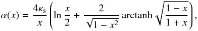 (8)from which the convergence and shear are derived. In the limit of κs ≲ 0.1, the typical scales corresponding to the strong lensing regime (e.g., the size of critical curve and caustics) are much smaller than unity. In this case high numerical precision is required to accurately compute lensing quantities, such as the shear and convergence. However, simple analytic expressions can be found in this regime by avoiding such numerical difficulties. Keeping the first terms in a series expansion of (8) for x ≪ 1 leads to
 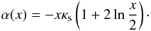 (9)In this case, the convergence and shear are given by
 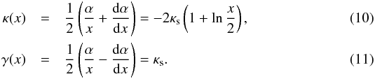 Allowing a relative deviation of less than 1% (0.1%) with respect to the exact expression, we found that Eq. (9) is a good approximation to the deflection angle for x ≤ 0.12 (x ≤ 0.04), while the same holds for Eqs. (10) and (11) for the convergence and shear for x ≤ 0.08 and x ≤ 0.05 (x ≤ 0.025 and x ≤ 0.015), respectively.
From Eq. (10) and fixing a value for the iso-convergence contour as κconst., the equation κ(x) = κconst. has the solution  (12)From Eqs. (5), (10), and (11) it follows that
  (13)such that the determinant of the Jacobian matrix is
  (14)The solutions for the tangential and radial critical curves follow from the equations above. The radial coordinates of these curves are3
 The expressions for the caustics are obtained straightforwardly by inserting the expressions above in the lens equation with the deflection angle given in Eq. (9). The validity of these solutions is discussed in Sect. 5.
3.2. Pseudo-elliptical NFW model
The construction of pseudo-elliptical models is made by replacing the radial coordinate of the lensing potential by  (17)where aϕ and bϕ are two parameters that define the lensing potential ellipticity. Adopting the approach of the angle deflection method introduced by Golse & Kneib (2002; see also Dúmet-Montoya et al. 2012, hereafter DCM), from Eqs. (9)–(11), the deflection angle, convergence, and components of the shear of the PNFW model are
 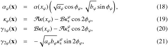 where
where  (22)and we denote the NFW characteristic convergence, Eq. (2), by
  .
.
From Eq. (19) and fixing a value for the iso-convergence contour as κconst., the equation κϕ(x) = κconst. has the solution 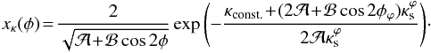 (23)Therefore, the iso-convergence contours are not elliptical, as is well known for pseudo-elliptical models.
The solutions for critical curves are a bit more involved. From Eqs. (19)–(21), the determinant of the Jacobian matrix is  (24)Then, solving the equation det J(x) = 0 for κ(xϕ), defining
  and inverting
  , using Eq. (17), we obtain
 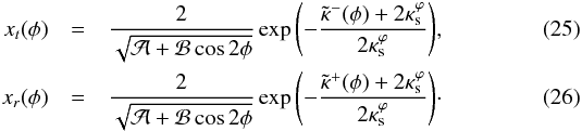 These curves are mapped onto the source plane by using the lens equation with the deflection angle given in Eq. (18). The validity of these solutions is discussed in Sect. 5.
3.3. Elliptical NFW model
We construct the ENFW model by replacing the radial coordinate of the surface mass density, Eq. (10), by 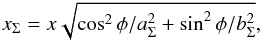 (27)where aΣ and bΣ define the ellipticity of the mass distribution.
The lensing functions of this model can be written as (see Appendix A) ![Mathematical equation: \begin{eqnarray} \alpha_{1\Sigma}(\vec{x}) & = & a_{\Sigma}b_{\Sigma} x\left[ \mathcal{J}_0\kappa(x)-2\kappa^\Sigma_{\rm s}\mathcal{L}_0(\phi)\right] \cos{\phi}, \label{alpha1_enfw} \\ \alpha_{2\Sigma}(\vec{x}) & = & a_{\Sigma}b_{\Sigma} x \left[\mathcal{J}_1\kappa(x)-2\kappa^\Sigma_{\rm s}\mathcal{L}_1(\phi)\right] \sin{\phi}, \label{alpha2_enfw} \\ \kappa_\Sigma(\vec{x})& \equiv &\kappa(x_\Sigma)=1-\frac{1}{2}\left[\mathcal{P} +\mathcal{Q}-a_{\Sigma}b_{\Sigma}(\mathcal{J}_0+\mathcal{J}_1)\kappa(x) \right], \label{kappa_enfw}\\ \gamma_{1\Sigma}(\vec{x})&=&\frac{1}{2}\left[a_{\Sigma}b_{\Sigma} (\mathcal{J}_0-\mathcal{J}_1)\kappa(x)+\mathcal{Q}-\mathcal{P}\right], \label{g1_enfw}\\ \gamma_{2\Sigma}(\vec{x})&=&-a_{\Sigma}b_{\Sigma}\kappa_{\rm s}^\Sigma\sin{2\phi}\mathcal{K}_1(\phi), \label{g2_enfw} \end{eqnarray}](/articles/aa/full_html/2013/12/aa21618-13/aa21618-13-eq69.png) where we denote the characteristic convergence, Eq. (2), by
where we denote the characteristic convergence, Eq. (2), by  and define
 ![Mathematical equation: \begin{eqnarray} \mathcal{P}&=&1+2a_{\Sigma}b_{\Sigma}\kappa_{\rm s}^\Sigma\left[\mathcal{K}_0(\phi)\cos^2{\phi}+\mathcal{L}_0(\phi) \right], \label{p_enfw}\\ \mathcal{Q}&=&1+2a_{\Sigma}b_{\Sigma}\kappa_{\rm s}^\Sigma \left[\mathcal{K}_2(\phi)\sin^2{\phi}+\mathcal{L}_1(\phi) \right]. \label{q_enfw} \end{eqnarray}](/articles/aa/full_html/2013/12/aa21618-13/aa21618-13-eq71.png) We computed the accuracy of Eqs. (28) and (29) with respect to the exact expressions (Eq. (A.1)) for the angles φ in which the deviations are maximal. For a percentile deviation less than 1% (0.1%), such expressions are good approximations of the exact components of the deflection angle for x ≤ 0.11 (x ≤ 0.03) and x ≤ 0.10 (x ≤ 0.025), respectively, within the ellipticity parameter range 0.1–0.6.
We computed the accuracy of Eqs. (28) and (29) with respect to the exact expressions (Eq. (A.1)) for the angles φ in which the deviations are maximal. For a percentile deviation less than 1% (0.1%), such expressions are good approximations of the exact components of the deflection angle for x ≤ 0.11 (x ≤ 0.03) and x ≤ 0.10 (x ≤ 0.025), respectively, within the ellipticity parameter range 0.1–0.6.
For an iso-convergence contour value κconst., the solution for κΣ(x) = κconst. is 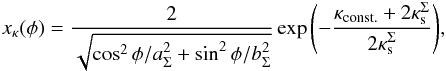 (35)which are ellipses, as expected.
From the definitions in (5) and Eqs. (30)–(32), the determinant of the Jacobian matrix is  (36)Following a similar procedure to obtain the critical curves for the PNFW model, the solutions of the equation det J(x) = 0 are
 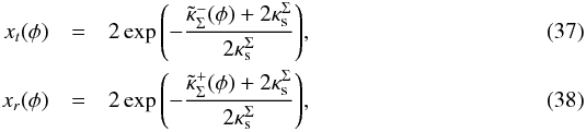 where we define
 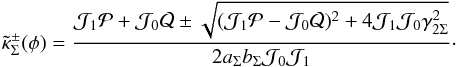 The corresponding caustics are obtained by using the lens equation with the deflection angle given in Eqs. (28) and (29). The validity of these solutions is discussed in Sect. 5.
4. Solutions for the deformation cross section
Gravitational arcs are usually defined as images with length-to-width ratio, L/W, greater than a threshold Rth. For fast calculations in arc statistics, it is useful to approximate L/W to the ratio of the eigenvalues of the Jacobian matrix (Wu & Hammer 1993; Bartelmann & Weiss 1994; Hamana & Futamase 1997)  (39)where Rλ = λr/λt. This approximation holds for infinitesimal circular sources and breaks down for arcs generated by the merger of multiple images (Rozo et al. 2008) or by large or noncircular sources.
In this section, using the approximation above, we derive analytical solutions for constant distortion curves for the NFW models (Sect. 4.1). We thereafter employ these solutions to compute the arc cross section (Sect. 4.2).
4.1. Constant distortion curves
A typical arc-forming region in the lens plane is determined by the so-called constant distortion curves, corresponding to the | Rλ | = Rth contours. An often used value for Rth is 10. As the value of Rth is decreased, the inner curve (corresponding to Rλ = −Rth) gets closer to the center, while the outer enclosing curve (Rλ = + Rth) reaches higher radii, where the analytic approximations derived in Sect. 3 are less accurate. Therefore by using a lower value of Rth to determine the limit of validity of these approximations, we are assuring they are even more accurate in the arc formation region. For this reason, we adopt Rth = 5 when we make the numerical comparisons to the exact solution throughout this paper.
From the approximations given in Sect. 3, it is possible to obtain analytical solutions for the radial coordinates of constant distortion curves. For the circular NFW model, from Eq. (13), the equation Rλ(x) = Rth has the solution 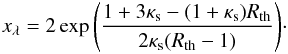 (40)For the PNFW model, calculating the radial coordinates of the constant distortion curves is a bit more complicated. From Eqs. (19)–(21), solving the equation
  for κ(xϕ), we obtain
  (41)where
  with
with  where φϕ is given in Eq. (22). Inverting Eq. (41) and using Eq. (17), we obtain for any angular position
  (42)Following the same procedure as above, for the ENFW model, from Eqs. (30)–(32), we obtain for each angular position
  (43)where we have defined
  with
with ![Mathematical equation: \begin{eqnarray*} \mathcal{R}_{1\Sigma} &=& \mathcal{P}+\mathcal{Q}+Q_{\rm th}(\mathcal{P}-\mathcal{Q}), \\ \mathcal{R}_{2\Sigma} &=& \mathcal{P}+\mathcal{Q}-Q_{\rm th}(\mathcal{P}-\mathcal{Q}), \\ Q_{1\Sigma} &=& a_\Sigma b_\Sigma[\mathcal{J}_0+\mathcal{J}_1+Q_{\rm th}(\mathcal{J}_0-\mathcal{J}_1)],\\ Q_{2\Sigma}& =& a_\Sigma b_\Sigma[\mathcal{J}_0+\mathcal{J}_1-Q_{\rm th}(\mathcal{J}_0-\mathcal{J}_1)], \end{eqnarray*}](/articles/aa/full_html/2013/12/aa21618-13/aa21618-13-eq98.png) where
where  ,
,  , and
, and  are given in Eqs. (33), (34), and (A.8), respectively.
In Eqs. (40), (42), and (43) the solution for the equation Rλ(x) = −Rth is obtained by replacing Rth by − Rth. Also, at the limits Rth → ∞ and Rth → 0, these expressions yield the radial coordinates of the tangential (Eqs. (15), (25), and (37)) and radial (Eqs. (16), (26), and (38)) critical curves of the corresponding models.
4.2. Arc cross section
The arc cross section, σRth, is defined as the weighted area in the source plane, such that sources within it will be mapped into arcs with L/W ≥ Rth. This cross section is usually computed using a large sample of arcs obtained from ray-tracing an even larger number of finite sources and is computationally demanding. An alternative for fast calculations is to use the approximation (39). In this case, the arc cross section is calculated in the lens plane as (Fedeli et al. 2006, DCM)  (44)where the quantity
  is known as (dimensionless) deformation cross section.
For low values of the characteristic convergences, the determinant of the Jacobian (see Eqs. (14), (24), and (36)) takes the form  where A, B, and C are independent of the radial coordinates. It is possible to reduce the calculation of (44) to a one-dimensional integral. Inserting the expression above into Eq. (44) and integrating over the radial coordinate, within the lower and upper limits given by the constant distortion curves (i.e., from − Rth to Rth), we obtain
 ![Mathematical equation: \begin{eqnarray} \tilde{\sigma}_{R_{\rm th}}=\frac{1}{2}\int_{0}^{2\pi}\left[\mathcal{S}(x_{+})+\mathcal{S}(x_{-})-2\mathcal{S}(x_t)\right]{\rm d}\phi \label{sigma_medio}, \end{eqnarray}](/articles/aa/full_html/2013/12/aa21618-13/aa21618-13-eq114.png) (45)where
(45)where  , is a function (given below) resulting from the integration of det J(x) over the radial coordinate, x± = x±(φ) are the solutions for the radial coordinate of the constant distortion curves for − Rth and Rth, and xt = xt(φ) is the solution for the radial coordinate of the tangential critical curve.
For the circular NFW model we have ![Mathematical equation: \begin{eqnarray} \mathcal{S}=x^2\left[1-\kappa_{\rm s}-\kappa(x)\right]^2, \end{eqnarray}](/articles/aa/full_html/2013/12/aa21618-13/aa21618-13-eq119.png) (46)such that Eq. (45) gives
(46)such that Eq. (45) gives ![Mathematical equation: \begin{eqnarray} \tilde{\sigma}_{R_{\rm th}}=\frac{4\pi\kappa^2_{\rm s}}{(R^2_{\rm th}-1)^2}\left[(R_{\rm th}+1)^2x^2_{+}+(R_{\rm th}-1)^2x^2_{-} \right] \label{dcs_nfw_analytic} \end{eqnarray}](/articles/aa/full_html/2013/12/aa21618-13/aa21618-13-eq120.png) (47)where x± are given in Eq. (40) for Rth and − Rth, respectively. This expression shows the exponential dependence of the cross section on κs (Caminha et al. 2013). For instance, varying κs from 0.01 to 0.1,
(47)where x± are given in Eq. (40) for Rth and − Rth, respectively. This expression shows the exponential dependence of the cross section on κs (Caminha et al. 2013). For instance, varying κs from 0.01 to 0.1,  changes approximately by 41 orders of magnitude. Further,
  for Rth ≫ 1 as expected from the behavior of sources near the caustics (Mollerach & Roulet 2002; Caminha et al. 2013).
For the PNFW model we have ![Mathematical equation: \begin{eqnarray} \mathcal{S}(\phi)=x^2\left[a_{\varphi} b_{\varphi} \mathcal{S}^{2}_{1\varphi}-(a_{\varphi} +b_{\varphi} )\mathcal{S}_{1\varphi}+\mathcal{S}_{0\varphi}\right], \label{S_pnfw} \end{eqnarray}](/articles/aa/full_html/2013/12/aa21618-13/aa21618-13-eq126.png) (48)where
(48)where  In this case, this function must be evaluated at xt and x± given in Eqs. (25) and (42), respectively.
For the ENFW model we have ![Mathematical equation: \begin{equation} \mathcal{S}(\phi)\!=\!x^2\left[(a_\Sigma b_\Sigma)^2(\mathcal{J}_0\mathcal{J}_1) \!\times\! \mathcal{S}^2_{1\Sigma}-a_\Sigma b_\Sigma(\mathcal{J}_1\mathcal{P}+\mathcal{J}_0\mathcal{Q})\mathcal{S}_{1\Sigma}\!+\!\mathcal{S}_{0\Sigma}\right], \label{S_enfw} \end{equation}](/articles/aa/full_html/2013/12/aa21618-13/aa21618-13-eq129.png) (49)with
(49)with 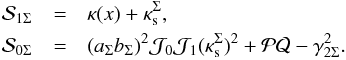 This function must be evaluated at xt, Eq. (37), and x± Eq. (43).
5. Domain of validity of the solutions
In this section we quantify the deviation of the analytic solutions (Sects. 3 and 4) with respect to their corresponding exact calculations, seeking to determine their domains of validity in terms of the model parameters (Sect. 5.1). Then, aiming to test the domain of validity of these solutions for computing other lensing quantities, we compare the deformation cross sections in Sect. 5.2.
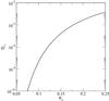 |
Fig. 1 Mean weighted squared radial fractional difference |
5.1. Limits for constant distortion curves and critical curves
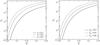 |
Fig. 2 Mean weighted squared radial fractional difference |
To compare the analytic solutions for critical curves and constant distortion curves to their exact calculations, we use as a figure-of-merit the mean weighted squared fractional difference between the two curves (Dúmet-Montoya et al. 2013) ![Mathematical equation: \begin{eqnarray} \mathcal{D}^2 = \frac{\sum_{i=1}^N w_i\left[x_{\rm ex}(\phi_i) - x_{\rm app}(\phi_i) \right]^2}{\sum_{i=1}^N w_i x^2_{\rm ex}(\phi_i)}, \label{D2_funct} \end{eqnarray}](/articles/aa/full_html/2013/12/aa21618-13/aa21618-13-eq133.png) (50)where N is the number of points of the curves, φi is their polar angle, wi = φi − φi − 1 is a weight (to account for a possible non-uniform distribution of points), xex(φi) and xapp(φi) are the radial coordinates of the curves curves obtained from the exact and approximated calculations, respectively. We notice that, the
(50)where N is the number of points of the curves, φi is their polar angle, wi = φi − φi − 1 is a weight (to account for a possible non-uniform distribution of points), xex(φi) and xapp(φi) are the radial coordinates of the curves curves obtained from the exact and approximated calculations, respectively. We notice that, the  in Eq. (50) is independent both on the lens length scale and on the discretization.
Choosing a maximum value for , we can define upper values for the characteristic convergences (for a given ellipticity) such that the contour curves obtained with both the exact and approximated calculations will be close enough to each other. This maximum value is chosen by visually comparing the approximated and exact solutions for critical curves and constant distortion curves for several values of and combinations of the NFW model parameters.
We compute on the Rλ = + Rth curves since their points are the farthest from the lens center. Thus, imposing a limit on the NFW parameters to match the Rλ = Rth curve, we automatically match the curves enclosed by it. We have checked that for a broad range of the NFW model parameters and ellipticities (for both elliptical and pseudo-elliptical models), a good visual matching of the exact and approximated curves if obtained for a maximum value of  (for Rth = 5). This value also ensures a good matching of the critical curves, and we found that the corresponding curves in the source plane are well-matched, too. We thus fix this as the upper value of throughout this work.
In Fig. 1 we show for the Rth = 5 curve as a function of κs for the circular NFW model. Setting the above upper value for leads to a maximum value of κs = 0.18, for which all curves | Rλ | = Rth ( ≥ 5), and the radial critical curves are well matched.
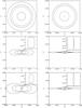 |
Fig. 3 Constant distortion curves Rλ = + Rth (dot-dashed lines), Rλ = −Rth (dot-dot-dashed lines) for Rth = 5, tangential curves (dashed lines), and radial curves (dash-dash-dotted lines) obtained with the exact (thick gray lines) and approximated (black lines) calculations in the lens plane (left panels) and source plane (right panels). Upper panels: NFW model for κs = 0.15. Middle panels: PNFW model for |

For the PNFW model, we chose the convention (Blandford & Kochanek 1987; Golse & Kneib 2002)  (51)where the ellipticity parameter ε is defined in the range 0 ≤ ε < 1. As shown in DCM, for low values of
  we must have ε ≲ 0.5 to avoid dumbbell-shape mass distributions. In the forthcoming analyses, we therefore adopt an upper value of ε = 0.5. In the left panel of Fig. 2 we show as a function of for some values of ε. For the higher value of ε considered, is reached for
  , providing an upper limit for the characteristic convergence for the validity of the approximations. However, higher values of are allowed as ε decreases. For instance, when ε → 0, we find that
  (in agreement with the result for the circular NFW model).
For the ENFW model, we chose the parametrization  (52)where the ellipticity εΣ is defined in the range 0 ≤ εΣ < 1. In the right hand panel of Fig. 2 we show as a function of
  for some values of εΣ. The behavior of , as well as the maximum values of εΣ for each , is qualitatively similar to that of the PNFW model. In this case, we find that a maximum value of
  is allowed for εΣ = 0.7. Again the maximum value
  as εΣ → 0.
In Appendix B we present fitting functions for the maximum values of ε (εΣ) as a function of () for which the approximation is accurate following the criteria of this section. In Fig. 3 we show the constant distortion curves (including tangential and radial critical curves) in both the lens and source planes, for some values of the NFW, PNFW, and ENFW parameters, both using the approximations introduced in this work, as well as through the numerical computation with no approximations. The parameters were chosen such that  , i.e. less than our cut
  . We see that the exact and approximated curves are almost indistinguishable, visually illustrating the validity of using to determine the domain of validity of the approximations.
5.2. Comparison between deformation cross sections
We compare the exact calculations and the solutions derived in Sect. 4.2, in order to verify that the limits derived in Sect. 5.1 also give a domain of validity for the deformation cross section. To quantify this comparison, we compute the relative difference  (53)where the subscripts ex and app refer to the exact and approximated calculations, respectively.
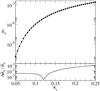 |
Fig. 4 Deformation cross section for the circular NFW lens model as a function of κs. Solid line corresponds to expression (47). Filled circles correspond to the exact (numerical) calculation. |
In Fig. 4 we show (upper panel) and  (bottom panel) as a function of κs for both the exact and approximated calculations. Considering the limit of the previous section, i.e., κs ≤ 0.18, Eq. (47) deviates from the exact calculation by at most 2.5%.
In the left panels of Fig. 5 we show (upper panel) and (bottom panel) as a function of for the PNFW model for both the exact and the approximated calculations. Considering the limit of applicability obtained in the previous section ( and ε ≤ 0.5), Eq. (45), with Eq. (48), deviates at most 2.6% from the exact calculation. A very similar result is found for the ENFW model. In this case, for
  and εΣ ≤ 0.7, we find that ( calculated by Eq. (45) with Eq. (49)) is at most 2.5%.
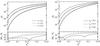 |
Fig. 5 Deformation cross sections for the PNFW model (left panel) and ENFW model (right panel). Symbols correspond to the exact calculations. |
6. Mapping among PNFW and ENFW parameters
As mentioned in the introduction, elliptical models are more physically motivated than pseudo-elliptical ones. However, determination of lensing quantities, such as the shear, for the former requires evaluating integrals (Schramm 1990; Keeton 2001a, see also Appendix A), which generally have to be computed numerically. On the other hand, pseudo-elliptical models do not require such integrals to be evaluated (see, e.g., Eqs. (18)–(21)) allowing for fast calculations for the same quantities. However, it is well known that pseudo-elliptical models have two main limitations: their surface mass density can assume negative values in some regions (Blandford & Kochanek 1987) and may present a “dumbbell” shape for high ellipticities (Kovner 1989; Schneider et al. 1992; Kassiola & Kovner 1993). At least in the case of the NFW model, the first problem does not affect the region of arc formation (DCM). Regarding the shape of the iso-convergence contours, for each value of , there is a range in ε for which the contours are approximately elliptical (DCM). In principle, within this range of parameters, the pseudo-elliptical models could be employed instead of elliptical ones in studies that require numerous evaluations of lensing quantities. For this sake, a correspondence among model parameters has to be established, which associates a pair of the PNFW parameters (ε,  ) to a pair of the ENFW ones (εΣ,
  ).
).
To obtain εΣ from the PNFW model we use the same procedure as in Golse & Kneib (2002, see also DCM). From Eq. (23) we define the semi-major axis a by xκ(φ = 0) and the semi-minor axis b by xκ(φ = π/2) such that ![Mathematical equation: \begin{eqnarray} \varepsilon_\Sigma = 1-\frac{b}{a} & = & 1-\sqrt{\frac{a_{\varphi} }{b_{\varphi} }}\exp{\left[\frac{(a_{\varphi} -b_{\varphi} )}{(a_{\varphi} +b_{\varphi} )} \right]}, \nonumber \\ & =& 1-\sqrt{\frac{1-\varepsilon}{1+\varepsilon}}\exp{\left[-\frac{\varepsilon}{2} \right]}\cdot \label{ellip_gk} \end{eqnarray}](/articles/aa/full_html/2013/12/aa21618-13/aa21618-13-eq181.png) (54)This expression has no dependence on Rth or on .
(54)This expression has no dependence on Rth or on .
The qualitative behavior of εΣ(ε) from this equation is very similar to what was found numerically for generic values of in DCM (see, e.g., their Fig. 6). For ε ≪ 1, the expression above gives εΣ ≃ 2ε, in agreement with DCM (see, e.g., Eq. (B.2), which gives εΣ = 1.97ε, for  ).
).
Interestingly, Eq. (54) is a good approximation of the exact relation for values of well above the limit of validity of the approximation derived in Sect. 5. Indeed, the relative deviation with respect to the exact calculation of  (see the elliptical fit method in Sect. 4 of DCM) is at most 5% for
  , with ε ≤ 0.5 and Rth ≥ 5.
To associate a value of to a pair (, ε), we require that the tangential critical curves of the PNFW and ENFW models match at φ = 0. This condition, from Eqs. (25) and (37), gives ![Mathematical equation: \begin{eqnarray} \kappa_{\rm s}^\Sigma=\frac{b_{\varphi} \kappa_{\rm s}^\varphi}{a_\Sigma b_\Sigma\left[\mathcal{J}_1 +b_{\varphi} \kappa^\varphi_{\rm s}(\mathcal{J}_1\log{a_{\varphi} }-\mathcal{J}_1-2\mathcal{L}_1(0))\right]}\cdot \label{ka_rela_gk} \end{eqnarray}](/articles/aa/full_html/2013/12/aa21618-13/aa21618-13-eq192.png) (55)For ε = εΣ = 0 the expression above reduces to
(55)For ε = εΣ = 0 the expression above reduces to  , as it should be.
We determine the upper value of such that the expression above deviates by at most 5% with respect to the exact calculation. This yields  for ε ≤ 0.5 and Rth ≥ 5. Again, the domain of validity of the approximate mapping is greater than for the lensing equations.
7. Summary and concluding remarks
When considering low values of the characteristic convergence of the NFW model (i.e., on the galactic and galaxy group mass scales), some strong lensing quantities require high numerical precision to yield accurate results, which can demand a lot of time. Motivated by this issue, we obtained analytic solutions for several strong lensing quantities for elliptical and pseudo-elliptical NFW models and quantified their corresponding limits of validity.
The starting point is approximation (8) for the deflection angle of the circular NFW model. This approximation was applied to the standard prescriptions for obtaining the convergence and shear for circular, elliptical, and pseudo-elliptical models, leading to analytic solutions for these quantities (Sect. 3). Those were in turn used to derive analytic expressions for iso-convergence contours and critical curves (see Sect. 3) and for the constant distortion curves as a function of Rth (Sect. 4.1).
As a practical application of these results, we computed the deformation cross section (σRth). In the case of the circular NFW model, we obtained an analytical formula for σRth (Eq. (47)), which reproduces the behavior with respect to κs and the scaling with Rth obtained numerically in previous works (see, e.g., Caminha et al. 2013). We have shown that the computation of this cross section is reduced to a one-dimensional integral for both the PNFW and ENFW models (Eq. (45) with either Eq. (48) or Eq. (49), respectively). These expressions speed up the numerical computations by two orders of magnitude for the PNFW model and one order of magnitude for the ENFW one, independently of the values of the ellipticity parameter.
We used the figure-of-merit , Eq. (50), to quantify the deviation of the solutions of the constant distortion curves with respect to their exact calculations. Setting a maximum value of , we find that Eqs. (42), (43), match its corresponding exact calculation up to  (
( ) for ε ≤ 0.5 (εΣ ≤ 0.7) and Rth > 5. In particular, we find that the characteristic convergence can go up to 0.18 as the ellipticity parameters tend to zero, as expected from the limit derived for the circular NFW model. In Appendix B we provide fitting functions for the maximum ellipticity allowed as a function of the characteristic convergences (in the range
  ) to ensure the validity of the approximations. We emphasize that these limits also ensure a good match for critical curves and the Rλ = −Rth curves to their corresponding exact calculations, since these curves are enclosed by the Rλ = Rth curve. We verified that the corresponding curves in the source plane also match the exact solution for the parameters within the limits derived above.
We compared the deformation cross sections (obtained from both the exact and approximated calculations) in order to check that the domain of validity derived for the constant distortion curves also holds for this quantity (Sect. 5.2), which we found to be the case. For instance, for the circular NFW model, for κs ≤ 0.18 and Rth = 5, Eq. (47) deviates at most 2.5% from the exact calculation, while for the PNFW and ENFW,  /
/ (Eq. (53)) is at most 2.5%, for and ε < 0.5, and
  and εΣ < 0.7, respectively.
Overall, the approximate solutions presented here are accurate for all strong lensing quantities that were addressed in this work, within the considered parameter ranges, for κs ≤ 0.1. In some cases they are valid for higher κs, such as for low ellitpcities. Furthermore, some derived quantities are valid up to much higher characteristic convergences. For example, the ellipticity of the iso-convergence contours of the PNFW model is reproduced well by the simple analytic form of Eq. (54) up to  . We found that in this range the relation εΣ(ε) is independent of and of the chosen value of the contour. To complete the association of the PNFW to ENFW model parameters we derived a relation among characteristic convergences, Eq. (55), which also matches the values obtained in DCM for
  and Rth ≥ 5.
The analytic solutions presented here allow for a robust and fast computation of several strong lensing quantities to be carried out in the low characteristic convergence regime. They may thus be useful for the lensing community and could be readily included in strong lensing codes, considering the domain of applicability derived in this work.
In principle, the approximate solutions derived in this paper could be extended to other quantities, such as the lensing magnification and the magnification cross section. They might also be applied to finding solutions of the lens equation, for multiple images and arcs. One way of finding approximate solutions for arcs, for low ellitpicities, is through the perturbative approach (Alard 2007, 2008; Peirani et al. 2008), for which the Einstein ring solution (given analytically in Eq. (15)) is the starting point. Therefore, analytic solutions for arcs might be derived in this framework. The investigation of these and other possible extensions is left for future work.
To obtain this value of κs we use the expressions in Caminha et al. (2013) with the same choices for the NFW and cosmological parameters as described in Sect. 2.2 of Dúmet-Montoya et al. (2012).
These solutions are shown in Meneghetti et al. (2003). However, there is a typo in this reference as they appear in their Eq. (11) as the eigenvalues of the Jacobian matrix.
Acknowledgments
We thank the anonymous referee for useful suggestions that helped improve this manuscript. We thank the anonymous referee of DCM for pushing us to consider the low κs regime. H. S. Dúmet-Montoya is funded by the Brazilian agency CNPq. G. B. Caminha is funded by CNPq and CAPES. M. Makler is partially supported by CNPq (grant 309804/2012-4) and FAPERJ (grant E-26/110.516/2012).
References
- Alard, C. 2007, MNRAS, 382, L58 [NASA ADS] [Google Scholar]
- Alard, C. 2008, MNRAS, 388, 375 [NASA ADS] [CrossRef] [Google Scholar]
- Annis, J., Bridle, S., Castander, F. J., et al. 2005 [arXiv:astro-ph/0510195] [Google Scholar]
- Asano, K. 2000, PASJ, 52, 99 [NASA ADS] [Google Scholar]
- Barkana, R. 1998, ApJ, 502, 531 [NASA ADS] [CrossRef] [Google Scholar]
- Barnabè, M., Czoske, O., Koopmans, L. V. E., Treu, T., & Bolton, A. S. 2011, MNRAS, 415, 2215 [NASA ADS] [CrossRef] [Google Scholar]
- Bartelmann, M. 1995, A&A, 299, 11 [NASA ADS] [Google Scholar]
- Bartelmann, M. 1996, A&A, 313, 697 [NASA ADS] [Google Scholar]
- Bartelmann, M., & Weiss, A. 1994, A&A, 287, 1 [NASA ADS] [Google Scholar]
- Bartelmann, M., Steinmetz, M., & Weiss, A. 1995, A&A, 297, 1 [NASA ADS] [Google Scholar]
- Bartelmann, M., Huss, A., Colberg, J. M., Jenkins, A., & Pearce, F. R. 1998, A&A, 330, 1 [NASA ADS] [Google Scholar]
- Bartelmann, M., Meneghetti, M., Perrotta, F., Baccigalupi, C., & Moscardini, L. 2003, A&A, 409, 449 [NASA ADS] [CrossRef] [EDP Sciences] [Google Scholar]
- Bayliss, M. B. 2012, ApJ, 744, 156 [NASA ADS] [CrossRef] [Google Scholar]
- Belokurov, V., Evans, N. W., Hewett, P. C., et al. 2009, MNRAS, 392, 104 [NASA ADS] [CrossRef] [Google Scholar]
- Blandford, R. D., & Kochanek, C. S. 1987, ApJ, 321, 658 [NASA ADS] [CrossRef] [Google Scholar]
- Bolton, A. S., Burles, S., Koopmans, L. V. E., Treu, T., & Moustakas, L. A. 2006, ApJ, 638, 703 [NASA ADS] [CrossRef] [Google Scholar]
- Cabanac, R. A., Alard, C., Dantel-Fort, M., et al. 2007, A&A, 461, 813 [NASA ADS] [CrossRef] [EDP Sciences] [Google Scholar]
- Caminha, G. B., Estrada, J., & Makler, M. 2013, ApJ, submitted [arXiv:1308.6569] [Google Scholar]
- Comerford, J. M., Meneghetti, M., Bartelmann, M., & Schirmer, M. 2006, ApJ, 642, 39 [NASA ADS] [CrossRef] [Google Scholar]
- Davis, A. N., Huterer, D., & Krauss, L. M. 2003, MNRAS, 344, 1029 [NASA ADS] [CrossRef] [Google Scholar]
- Dúmet-Montoya, H. S., Caminha, G. B., & Makler, M. 2012, A&A, 544, A83 (DCM) [NASA ADS] [CrossRef] [EDP Sciences] [Google Scholar]
- Dúmet-Montoya, H. S., Caminha, G. B., Moraes, B., et al. 2013, MNRAS, 433, 2975 [NASA ADS] [CrossRef] [Google Scholar]
- Ebeling, H., Edge, A. C., & Henry, J. P. 2001, ApJ, 553, 668 [Google Scholar]
- Estrada, J., Annis, J., Diehl, H. T., et al. 2007, ApJ, 660, 1176 [NASA ADS] [CrossRef] [Google Scholar]
- Fassnacht, C. D., Moustakas, L. A., Casertano, S., et al. 2004, ApJ, 600, L155 [NASA ADS] [CrossRef] [Google Scholar]
- Faure, C., Kneib, J.-P., Covone, G., et al. 2008, ApJS, 176, 19, Erratum 2008, 178, 382 [NASA ADS] [CrossRef] [Google Scholar]
- Fedeli, C., Meneghetti, M., Bartelmann, M., Dolag, K., & Moscardini, L. 2006, A&A, 447, 419 [NASA ADS] [CrossRef] [EDP Sciences] [Google Scholar]
- Furlanetto, C., Santiago, B. X., Makler, M., et al. 2013, MNRAS, 432, 73 [NASA ADS] [CrossRef] [Google Scholar]
- Gilbank, D. G., Gladders, M. D., Yee, H. K. C., & Hsieh, B. C. 2011, AJ, 141, 94 [NASA ADS] [CrossRef] [Google Scholar]
- Gladders, M. D., Hoekstra, H., Yee, H. K. C., Hall, P. B., & Barrientos, L. F. 2003, ApJ, 593, 48 [NASA ADS] [CrossRef] [Google Scholar]
- Golse, G., & Kneib, J.-P. 2002, A&A, 390, 821 [NASA ADS] [CrossRef] [EDP Sciences] [Google Scholar]
- Golse, G., Kneib, J.-P., & Soucail, G. 2002, A&A, 387, 788 [NASA ADS] [CrossRef] [EDP Sciences] [Google Scholar]
- Grossman, S. A., & Saha, P. 1994, ApJ, 431, 74 [NASA ADS] [CrossRef] [Google Scholar]
- Hamana, T., & Futamase, T. 1997, MNRAS, 286, L7 [NASA ADS] [CrossRef] [Google Scholar]
- Hattori, M., Watanabe, K., & Yamashita, K. 1997, A&A, 319, 764 [NASA ADS] [Google Scholar]
- Hennawi, J. F., Gladders, M. D., Oguri, M., et al. 2008, AJ, 135, 664 [NASA ADS] [CrossRef] [Google Scholar]
- Horesh, A., Maoz, D., Hilbert, S., & Bartelmann, M. 2011, MNRAS, 418, 54 [NASA ADS] [CrossRef] [Google Scholar]
- Jackson, N. 2008, MNRAS, 389, 1311 [NASA ADS] [CrossRef] [Google Scholar]
- Jing, Y. P., & Suto, Y. 2002, ApJ, 574, 538 [NASA ADS] [CrossRef] [Google Scholar]
- Jullo, E., Kneib, J.-P., Limousin, M., et al. 2007, New J. Phys., 9, 447 [Google Scholar]
- Jullo, E., Natarajan, P., Kneib, J.-P., et al. 2010, Science, 329, 924 [NASA ADS] [CrossRef] [PubMed] [Google Scholar]
- Kassiola, A., & Kovner, I. 1993, ApJ, 417, 450 [NASA ADS] [CrossRef] [Google Scholar]
- Kausch, W., Schindler, S., Erben, T., Wambsganss, J., & Schwope, A. 2010, A&A, 513, A8 [NASA ADS] [CrossRef] [EDP Sciences] [Google Scholar]
- Keeton, C. R. 2001a [arXiv:astro-ph/0102341] [Google Scholar]
- Keeton, C. R. 2001b [arXiv:astro-ph/0102340] [Google Scholar]
- Kneib, J.-P. 2002, in Proc. The shapes of galaxies and their dark halos, ed. P. Natarajan, 50 [Google Scholar]
- Kneib, J. P., Mellier, Y., Fort, B., & Mathez, G. 1993, A&A, 273, 367 [NASA ADS] [Google Scholar]
- Kneib, J.-P., Van Waerbeke, L., Makler, M., & Leauthaud, A. 2010, CFHT programs 10BF023, 10BC02, 10BB009 [Google Scholar]
- Koopmans, L. V. E., Bolton, A., Treu, T., et al. 2009, ApJ, 703, L51 [NASA ADS] [CrossRef] [Google Scholar]
- Kovner, I. 1989, ApJ, 337, 621 [NASA ADS] [CrossRef] [Google Scholar]
- Kubo, J. M., & Dell’Antonio, I. P. 2008, MNRAS, 385, 918 [NASA ADS] [CrossRef] [Google Scholar]
- Kubo, J. M., Allam, S. S., Drabek, E., et al. 2010, ApJ, 724, L137 [NASA ADS] [CrossRef] [Google Scholar]
- Ludlow, A. D., Navarro, J. F., Boylan-Kolchin, M., et al. 2013, MNRAS, 432, 1103 [NASA ADS] [CrossRef] [Google Scholar]
- Luppino, G. A., Gioia, I. M., Hammer, F., Le Fèvre, O., & Annis, J. A. 1999, A&AS, 136, 117 [NASA ADS] [CrossRef] [EDP Sciences] [Google Scholar]
- Macciò, A. V., Dutton, A. A., van den Bosch, F. C., et al. 2007, MNRAS, 378, 55 [NASA ADS] [CrossRef] [Google Scholar]
- Meneghetti, M., Bartelmann, M., & Moscardini, L. 2003, MNRAS, 340, 105 [NASA ADS] [CrossRef] [Google Scholar]
- Meneghetti, M., Baccigalupi, C., Bartelmann, M., et al. 2005, in Gravitational lensing impact on cosmology, eds. Y. Mellier & G. Meylan, IAU Symp., 225, 185 [Google Scholar]
- Miralda-Escude, J. 1993, ApJ, 403, 497 [NASA ADS] [CrossRef] [Google Scholar]
- Mollerach, S., & Roulet, E. 2002, Gravitational lensing and microlensing (World Scientific Publishing Co. Pte. Ltd.) [Google Scholar]
- More, A., Cabanac, R., More, S., et al. 2012, ApJ, 749, 38 [Google Scholar]
- Moustakas, L. A., Marshall, P., Newman, J. A., et al. 2007, ApJ, 660, L31 [NASA ADS] [CrossRef] [Google Scholar]
- Navarro, J. F., Frenk, C. S., & White, S. D. M. 1996, ApJ, 462, 563 [NASA ADS] [CrossRef] [Google Scholar]
- Navarro, J. F., Frenk, C. S., & White, S. D. M. 1997, ApJ, 490, 493 [NASA ADS] [CrossRef] [Google Scholar]
- Oguri, M., Lee, J., & Suto, Y. 2003, ApJ, 599, 7, Erratum 2004, 608, 1175 [NASA ADS] [CrossRef] [Google Scholar]
- Peirani, S., Alard, C., Pichon, C., Gavazzi, R., & Aubert, D. 2008, MNRAS, 390, 945 [NASA ADS] [CrossRef] [Google Scholar]
- Petters, A. O., Levine, H., & Wambsganss, J. 2001, Singularity theory and gravitational lensing (Berlin: Birkhäuser) [Google Scholar]
- Postman, M., Coe, D., Benítez, N., et al. 2012, ApJS, 199, 25 [NASA ADS] [CrossRef] [Google Scholar]
- Ratnatunga, K. U., Griffiths, R. E., & Ostrander, E. J. 1999, AJ, 117, 2010 [NASA ADS] [CrossRef] [Google Scholar]
- Rozo, E., Nagai, D., Keeton, C., & Kravtsov, A. 2008, ApJ, 687, 22 [NASA ADS] [CrossRef] [Google Scholar]
- Sand, D. J., Treu, T., Ellis, R. S., & Smith, G. P. 2005, ApJ, 627, 32 [NASA ADS] [CrossRef] [Google Scholar]
- Schneider, P., Ehlers, J., & Falco, E. E. 1992, Gravitational lenses (Berlin: Springer-Verlag) [Google Scholar]
- Schramm, T. 1990, A&A, 231, 19 [NASA ADS] [Google Scholar]
- Smith, G. P., Kneib, J.-P., Smail, I., et al. 2005, MNRAS, 359, 417 [NASA ADS] [CrossRef] [Google Scholar]
- Suyu, S. H., Hensel, S. W., McKean, J. P., et al. 2012, ApJ, 750, 10 [NASA ADS] [CrossRef] [Google Scholar]
- Vegetti, S., & Koopmans, L. V. E. 2009, MNRAS, 392, 945 [NASA ADS] [CrossRef] [Google Scholar]
- Wayth, R. B., & Webster, R. L. 2006, MNRAS, 372, 1187 [NASA ADS] [CrossRef] [Google Scholar]
- Wen, Z.-L., Han, J.-L., & Jiang, Y.-Y. 2011, RA&A, 11, 1185 [Google Scholar]
- Wiesner, M. P., Lin, H., Allam, S. S., et al. 2012, ApJ, 761, 1 [NASA ADS] [CrossRef] [Google Scholar]
- Willis, J. P., Hewett, P. C., Warren, S. J., Dye, S., & Maddox, N. 2006, MNRAS, 369, 1521 [NASA ADS] [CrossRef] [Google Scholar]
- Wu, X.-P., & Hammer, F. 1993, MNRAS, 262, 187 [NASA ADS] [CrossRef] [Google Scholar]
- Zaritsky, D., & Gonzalez, A. H. 2003, ApJ, 584, 691 [NASA ADS] [CrossRef] [Google Scholar]
Appendix A: Lensing functions for elliptical lens models
The lensing functions of models with elliptical mass distribution can be obtained following the expressions derived in Schramm (1990) and Keeton (2001a), which were generalized for any choice of the ellipticity parameterization in Caminha et al. (2013) and are given by  where aΣ and bΣ are defined in Eq. (27),
 ![Mathematical equation: \appendix \setcounter{section}{1} \begin{eqnarray} J_n := \int_0^1 \frac{\kappa(m(u))}{[1 - (1 - b^2_\Sigma)u]^{1/2 + n}[1 - (1 - a^2_\Sigma)u]^{3/2 - n}} \end{eqnarray}](/articles/aa/full_html/2013/12/aa21618-13/aa21618-13-eq216.png) (A.5)and
(A.5)and ![Mathematical equation: \appendix \setcounter{section}{1} \begin{eqnarray} K_n := \int_0^1 \frac{u\kappa^\prime(m(u))}{[1 - (1 - b^2_\Sigma)u]^{1/2 + n}[1 - (1 - a^2_\Sigma)u]^{5/2 - n}}, \end{eqnarray}](/articles/aa/full_html/2013/12/aa21618-13/aa21618-13-eq217.png) (A.6)where κ is the convergence of the circular model,
(A.6)where κ is the convergence of the circular model,  and we have defined the variable m2 = x2g(u,φ) such that
  For the ENFW model, with the approximation (10), we can rewrite the potential derivatives as
  (A.7)where
 ![Mathematical equation: \appendix \setcounter{section}{1} \begin{eqnarray} \mathcal{J}_n &=& \int_0^1 \frac{{\rm d}u}{[1 - (1 - b^2_\Sigma)u]^{1/2 + n}[1 - (1 - a^2_\Sigma)u]^{3/2 - n}}, \label{an_enfw}\\ \mathcal{K}_n(\phi) &=&\int_0^1 \frac{ug(\phi,u)^{-2}{\rm d}u}{[1 - (1 - b^2_\Sigma)u]^{1/2 + n}[1 - (1 - a^2_\Sigma)u]^{5/2 - n}}\cdot \label{dn_enfw} \\ \mathcal{L}_n(\phi) &=&\int_0^1 \frac{\log{g(\phi, u) {\rm d}u}}{[1 - (1 - b^2_\Sigma)u]^{1/2 + n}[1 - (1 - a^2_\Sigma)u]^{3/2 - n}}, \label{bn_enfw} \label{Ln} \end{eqnarray}](/articles/aa/full_html/2013/12/aa21618-13/aa21618-13-eq223.png) Substituting the expressions above in Eq. (A.1) we obtain Eqs. (28) and (29). Similarly, by substituting Eqs. (A.7)–(A.10) in (A.2)–(A.4) and using the definitions (6) and (7) we obtain Eqs. (30)–(32).
Substituting the expressions above in Eq. (A.1) we obtain Eqs. (28) and (29). Similarly, by substituting Eqs. (A.7)–(A.10) in (A.2)–(A.4) and using the definitions (6) and (7) we obtain Eqs. (30)–(32).
Appendix B: Fitting functions
Results from the regression analysis using the Padé approximant for  .
.
Applying the procedure outlined in Sect. 5.1, we obtained the maximum values of ε (εΣ) as a function of () such that the analytic solutions derived in the paper are accurate. We find that these functions are well fitted by a Padé approximant of the form  (B.1)where
  and κs correspond either to
  (for the PNFW) or
  (for the ENFW), and the values of coefficients are given in Table B.1.
All Tables
All Figures
|
Fig. 1 Mean weighted squared radial fractional difference |
| In the text | |
|
Fig. 2 Mean weighted squared radial fractional difference |
| In the text | |
|
Fig. 3 Constant distortion curves Rλ = + Rth (dot-dashed lines), Rλ = −Rth (dot-dot-dashed lines) for Rth = 5, tangential curves (dashed lines), and radial curves (dash-dash-dotted lines) obtained with the exact (thick gray lines) and approximated (black lines) calculations in the lens plane (left panels) and source plane (right panels). Upper panels: NFW model for κs = 0.15. Middle panels: PNFW model for |
| In the text | |
|
Fig. 4 Deformation cross section for the circular NFW lens model as a function of κs. Solid line corresponds to expression (47). Filled circles correspond to the exact (numerical) calculation. |
| In the text | |
|
Fig. 5 Deformation cross sections for the PNFW model (left panel) and ENFW model (right panel). Symbols correspond to the exact calculations. |
| In the text | |
Current usage metrics show cumulative count of Article Views (full-text article views including HTML views, PDF and ePub downloads, according to the available data) and Abstracts Views on Vision4Press platform.
Data correspond to usage on the plateform after 2015. The current usage metrics is available 48-96 hours after online publication and is updated daily on week days.
Initial download of the metrics may take a while.