| Issue |
A&A
Volume 560, December 2013
|
|
|---|---|---|
| Article Number | A70 | |
| Number of page(s) | 14 | |
| Section | Extragalactic astronomy | |
| DOI | https://doi.org/10.1051/0004-6361/201321284 | |
| Published online | 06 December 2013 | |
The unusual afterglow of the gamma-ray burst 100621A⋆,⋆⋆
1 Max-Planck-Institut für extraterrestrische Physik, Giessenbachstrasse 1, 85748 Garching, Germany
e-mail: This email address is being protected from spambots. You need JavaScript enabled to view it.
2 Dark Cosmology Centre, Niels Bohr Institute, University of Copenhagen, Juliane Maries Vej 30, 2100 Copenhagen, Denmark
3 Universitá degli studi di Milano-Bicocca, Piazza della Scienza 3, 20126 Milano, Italy
4 Institute of Experimental and Applied Physics, Czech Technical University in Prague, Horska 3a/22, 128 00 Prague 2, Czech Republic
5 International Centre for Radio Astronomy Research, Curtin University, GPO Box U1987, Perth, WA 6845, Australia
6 Shanghai Astronomical Observatory, Chinese Academy of Sciences (SHAO), 80 Nandan Road, 200030 Shanghai, PR China
7 ESO, Alonso de Córdoba 3107, Vitacura, Casilla 19001, Santiago, Chile
8 ALMA JAO, Alonso de Cordova 3107, Vitacura, Casilla 19001, Santiago, Chile
9 Thüringer Landessternwarte Tautenburg, Sternwarte 5, 07778 Tautenburg, Germany
10 American River College, Physics Dept., 4700 College Oak Drive, Sacramento, CA 95841, USA
11 Argelander-Institut für Astronomie, Auf dem Hügel 71, 53121 Bonn, Germany
12 Max-Planck-Institut für Radioastronomie, Auf dem Hügel 69, 53121 Bonn, Germany
13 European Southern Observatory, Schwarzschild-Str. 2, 85748 Garching, Germany
14 Roger Williams Univ., One Old Ferry Road, Bristol, RI 02809, USA
15 CSIRO Astronomy & Space Science, Locked Bag 194, Narrabri, NSW 2390, Australia
Received: 13 February 2013
Accepted: 17 April 2013
Abstract
Aims. With the afterglow of GRB 100621A being the brightest detected so far in X-rays, and superb GROND coverage in the optical/near-infrared during the first few hours, an observational verification of basic fireball predictions seemed possible.
Methods. In order to constrain the broad-band spectral energy distribution of the afterglow of GRB 100621A, dedicated observations were performed in the optical/near-infrared with the 7-channel Gamma-Ray Burst Optical and Near-infrared Detector (GROND) at the 2.2 m MPG/ESO telescope, in the sub-millimeter band with the large bolometer array LABOCA at APEX, and at radio frequencies with ATCA. Utilizing also Swift X-ray observations, we attempt an interpretation of the observational data within the fireball scenario.
Results. The afterglow of GRB 100621A shows a very complex temporal and spectral evolution. We identify three different emission components, the most spectacular one causing a sudden intensity jump about one hour after the prompt emission. The spectrum of this component is much steeper than the canonical afterglow. We interpret this component using a two-shell collision prescription after the first shell has been decelerated by the circumburst medium. We use the fireball scenario to derive constraints on the microphysical parameters of the first shell. Long-term energy injection into a narrow jet seems to provide an adequate description. Another noteworthy result is the large (AV = 3.6 mag) line-of-sight host extinction of the afterglow in an otherwise extremely blue host galaxy.
Conclusions. Some GRB afterglows have shown complex features, and that of GRB 100621A is another good example. Yet, detailed observational campaigns of the brightest afterglows promise to deepen our understanding of the formation of afterglows and the subsequent interaction with the circumburst medium.
Key words: gamma-ray burst: general / gamma-ray burst: individual: GRB 100621A / techniques: photometric
Based on data acquired with the Atacama Pathfinder Experiment (APEX) under ESO programme 285.D-5035(A).
Tables of the photometry are only available at the CDS via anonymous ftp to cdsarc.u-strasbg.fr (130.79.128.5) or via http://cdsarc.u-strasbg.fr/viz-bin/qcat?J/A+A/560/A70
© ESO, 2013
1. Introduction
1.1. The fireball scenario
Gamma-ray bursts (GRBs) are generally accepted to be related to the death of massive stars. Because of their large gamma-ray luminosity, GRBs can be detected to very high redshift, and thus provide a unique probe into the early universe. Understanding the emission mechanism and geometry is crucial for deriving the burst energetics and number density, and observing and understanding the afterglow emission is of the utmost importance for deciphering the burst environmental properties (e.g. gas density profile, metallicity, dust), as well as for deriving constraints on the progenitor (e.g. mass, rotation, binarity, supernova relation).
The late emission at X-ray to optical/radio wavelengths, the so-called afterglow, is dominated by synchrotron emission from the external shock, i.e. emission from relativistic electrons gyrating in a magnetic field (Meszaros & Rees 1997; Wijers et al. 1997; Wijers & Galama 1999). This synchrotron shock model is widely accepted as the major radiation mechanism in the external shock, and the macroscopic properties of these shocks are largely understood. Under the implicit assumptions that the electrons are Fermi accelerated at the relativistic shocks to a power-law distribution with an index p upon acceleration, their dynamics can be expressed in terms of four main parameters: (1) the total internal energy in the shocked region as released in the explosion; (2) the electron density and radial profile of the surrounding medium; (3) fraction of the shock energy going into the ISM electrons ϵe; and (4) the fraction of energy density in the magnetic field ϵB. Measuring the energetics and the energy partition (ϵe/ϵB) was possible only for a handful of the more than 900 GRB afterglows so far, as it requires truly multi-wavelength observations between X-rays and radio frequencies. Moreover, there are large uncertainties in the microphysics. How are the relativistic particles accelerated? How is the magnetic field in the shocked region generated? What is its structure and evolution? Addressing these questions is even more challenging.
According to standard synchrotron theory, the radiation power of an electron with co-moving energy γemc2 is  , so that high energy electrons cool more rapidly. For a continuous injection of electrons, which is the case for ongoing plowing of the forward shock into the interstellar medium (ISM), there is a break in the electron spectrum, above which the spectrum is steepened because of cooling. This energy is time-dependent, so this frequency break moves to lower energies for the ISM case and higher energies for a wind medium. Since the spectral slope and the temporal decay slope are identical for the two density profiles, it is the direction of the cooling break movement that allows us to distinguish between ISM and wind density profile surrounding the GRB.
Besides the cooling frequency νc, there is the injection frequency νm, corresponding to the electrons accelerated in the shock to a power-law distribution with a minimum Lorentz factor, and the self-absorption frequency, νsa. The final GRB afterglow spectrum is thus a four-segment broken power law (Meszaros et al. 1998; Sari et al. 1998) separated by νsa, νm, and νc. The order of νm and νc defines two types of spectra, namely the slow cooling case with νm < νc, and the fast cooling case νm > νc. For each case, and depending on wind vs. ISM density profile, theory predicts different slopes of the power-law segments and speeds at which νm and νc should be moving (Sari 1999). For standard parameters, νm should be moving from 1014 Hz to 1012 Hz within the first day, and νc from 1017 Hz to 1014 Hz. Because of sensitivity limitations in the sub-mm range, and lack of coordinated multi-wavelength observations, there is not a single GRB data set sufficient (in terms of wavelength and temporal coverage) to unambiguously verify these predictions for both frequencies, and just two GRBs where the high-frequency break (interpreted as cooling break) has been unambiguously shown to move (Blustin et al. 2006; Filgas et al. 2012).
1.2. GROND and GRB 100621A
The GROND instrument, a simultaneous 7-channel optical/near-infrared imager (Greiner et al. 2008) mounted at the 2.2 m telescope of the Max-Planck-Gesellschaft (MPG), operated by MPG and ESO (European Southern Observatory) at La Silla, Chile, started operation in May 2007. Built as a dedicated GRB follow-up instrument, GROND has observed basically every GRB visible from La Silla (weather allowing) since April 2008. The spectral energy distribution (SED) obtained with GROND between 400−2400 nm allows us to not only find high-z candidates (Greiner et al. 2009a; Krühler et al. 2011a), but also to measure the extinction and the power-law slope (Greiner et al. 2011). In the majority of all cases, this allows for a relatively accurate extrapolation of the SED into the sub-mm band, and consequently a prediction of the flux for sub-mm instruments, provided that νm has already passed the sub-mm band (which will be shown to be the case for the majority of GRBs after about one day).
 |
Fig. 1 GROND i′-band finding chart of GRB 100621A, including the photometric comparison stars (roman and arabic letters). North is up, and east to the left. |
Gamma-ray burst 100621A triggered the Burst Alert Telescope (BAT) on the Swift satellite (Gehrels et al. 2004) on June 21, 2010 at To = 03:03:32 UT (Ukwatta et al. 2010a). The prompt emission consists of a bright (25 000 cts/s peak count rate in the 15−350 keV band), smooth, triple-peak burst with a duration of nearly 70 s. Swift slewed immediately and started taking data with the XRT and UVOT telescopes at 76 s after the trigger. A bright X-ray afterglow was found at RA (2000.0) = 21h01m13.s24, Dec (2000.0) = −51°06′21.′′7 with an error radius of 1.′′7 (Evans et al. 2010). In fact, GRB 100621A had the brightest X-ray afterglow ever detected: with an initial count rate in excess of ≈140 000 cts/s, it saturated the XRT CCD for several minutes. Starting 80 seconds after the burst, the X-ray light curve in the 0.3−10 keV band can be modelled with four power laws1, with decay indices and temporal breaks as follows: α1 = 3.87 ± 0.02, tbreak1 = 439 ± 10 s,  ,
,  ks, α3 = 1.0 ± 0.1,
  ks, and α4 = 1.73 ± 0.08 (Ukwatta et al. 2010b).
Gamma-ray burst 100621A was also detected with INTEGRAL/SPI-ACS2 and Konus-Wind, providing a time-integrated spectrum with best-fit low-energy power-law index − 1.7, high-energy index − 2.45, and a peak energy  keV (Golenetskii et al. 2010). At z = 0.54 and standard cosmology (Ho = 70 km s-1 Mpc-1, ΩM = 0.27, ΩΛ = 0.73), this implies an isotropic energy release of Eiso = (2.8 ± 0.3) × 1052 erg (Golenetskii et al. 2010).
Initially, no UVOT counterpart was detected, and also rapid ground-based imaging with robotic telescopes (like ROTSE, Pandey et al. 2010) did not find an afterglow. Prompted by the discovery of a very red afterglow with GROND (Updike et al. 2010, but see below), a spectrum taken with X-Shooter at the VLT determined a redshift of z = 0.542 (Milvang-Jensen et al. 2010), and also faint UVOT detections were recovered (Ukwatta et al. 2010b).
Here, we describe our multi-wavelength observations and results for GRB 100621A, and present an analysis of the data in the framework of the fireball scenario.
2. Observations
Secondary standards used for the GROND data.
APEX/LABOCA observations at 345 GHz in photometry mode.
ATCA observations.
2.1. GROND observations
 |
Fig. 2 Afterglow light curve of GRB 100621A as observed with Swift in X-rays (top) and GROND in its seven filter bands (bottom). The J-band data points at 14 ks are from SOFI imaging, and the HKs-band data at 20 ks from a GROND observation in morning twilight at which the J-band was already saturated by the rising Sun. The seven vertical lines mark the times at which spectral energy distributions have been extracted (see text and Fig. 3). |
 |
Fig. 3 Multi-epoch SEDs (different colours) of the late-time afterglow of GRB 100621A as measured by Swift/XRT (right; not NH-corrected), GROND (middle; not AV-corrected)), APEX/LABOCA (middle left), and ATCA (far left), together with a broad-band model which fits all data available for the given epoch. The times of these SEDs are marked with vertical lines in Fig. 2, and the resulting break energies given in Table 4. Since the optical/NIR and X-ray fluxes in epochs 1−3 are very similar, epoch 3 (jump component at 6.8 ks) has been scaled upwards by a factor of 20, and epoch 2 (flares) down-scaled by a factor of 4. The curvature in the GROND data is due to strong extinction of the afterglow light in the host galaxy (dotted line). The breaks seemingly show erratic variations in frequency – see text for an interpretation. We do not consider the fits in this plot to be the final physical interpretation of the data, as it links emission components at different wavelength regions that do not belong together (see text). |
Some of the GROND data of this burst, in particular the J-band light curve and the host measurements, have already been reported in (Krühler et al. 2011b). Here, we report the full data set, including the multi-band light curve, and the SED evolution.
Exposures with GROND automatically started 230 s after the Swift trigger, one of the fastest reactions of 2.2 m/GROND so far. Simultaneous imaging in g′r′i′z′JHKs continued for 3.05 h, and was resumed on nights 2, 4, and 10 after the burst. The GROND data have been reduced in the standard manner using pyraf/IRAF (Tody 1993; Küpcü Yoldaş et al. 2008b). The optical/near-infrared (NIR) imaging was calibrated against the primary SDSS3 standard star network, or cataloged magnitudes of field stars from the SDSS in the case of g′r′i′z′ observations or the 2MASS catalog for JHKS imaging. This results in typical absolute accuracies of ±0.03 mag in g′r′i′z′ and ±0.05 mag in JHKS. The light curve of the GRB 100621A afterglow in all seven GROND filters is shown in Fig. 2.
2.2. Swift XRT data
Swift/XRT data have been reduced using the XRT pipeline provided by the Swift team. The X-ray spectra were flux-normalized to the epoch corresponding to the GROND observations using the XRT light curves from Evans et al. (2007, 2009). We then combined XRT and Galactic foreground extinction (E(B − V) = 0.03 mag; Schlegel et al. 1998) corrected GROND data to establish broad-band spectral energy distributions which are shown in Fig. 3.
2.3. NTT observations
The Son of ISAAC (SOFI) instrument on the New Technology Telescope (NTT) at La Silla was used to obtain NIR-spectroscopy. After recognizing the sharp drop in intensity at about To + 10 ks, we took four 60-s J-band images starting at 07:05 UT, on 21 Jun. 2010. While the results of the spectroscopy are deferred to a later publication (they are of no relevance to this paper), the imaging provides an additional photometric data point at a time when GROND observations were not longer possible because of visitor mode regulations. The SOFI images were reduced in the same manner as the GROND JHK data (actually within the same GROND pipeline), and calibrated against the 2MASS catalog.
2.4. APEX observations
Since the SED slope was steep, even after extinction correction, the predicted sub-mm flux density of ≈50 mJy at 1 day after the GRB led us to submit a director’s discretional time (DDT) proposal to ESO for observations with LABOCA (Siringo et al. 2009) on the Atacama Pathfinder Experiment (APEX)4 which was accepted at very short turn-around time.
The Large APEX Bolometer Camera LABOCA is an array of 295 composite bolometers. The system is optimized to work at the central frequency of 345 GHz with a bandwidth of about 60 GHz.
The first APEX/LABOCA observation was obtained 1.08 days after the GRB, leading to a clear detection. Two additional observations were performed at 2 days (another clear detection) and 4 days (upper limit only) after the GRB. This makes GRB 100621A one of the rare cases with a sub-mm light curve (see Sect. 5.3). These observations were all carried out in photometry mode.
Immediately after the first epoch observation (done in photometry mode), at 5:32−6:26 UT we obtained a complementary observation of GRB 100621A in mapping mode, for an exposure of 7 × 420 s and reaching a 1σ sensitivity of 14 mJy/beam. While no source was detected in this less sensitive observing mode, it verifies that there is no strong, unrelated source close to the GRB position, which otherwise could cause problems with the photometry mode data.
Reduction of the photometric data was done with the software BoA (Schuller 2012) using standard routines for photometry mode. Subscans were checked individually before averaging them in order to identify and remove outliers. The raster map was reduced with the CRUSH (Kovács 2008) software package. Flux density calibration was done against Neptune, G45.1, and B13134.
2.5. ATCA observations
In response to the initial detections of a bright afterglow of GRB 100621A (Ukwatta et al. 2010a; Evans et al. 2010; Updike et al. 2010; Milvang-Jensen et al. 2010), we also initiated observations of GRB 100621A with the Australia Telescope Compact Array (ATCA) in Narrabri, Australia, at the frequencies of 5.5 and 9.0 GHz with an observing bandwidth of 2 GHz. The observation sessions were carried out between June 24−26 and July 17−18 2010. The radio counterpart of the afterglow of GRB 100621A was detected during the sessions carried out in June 2010 at both 5.5 and 9.0 GHz at a position coincident with those of the X-ray and optical counterparts, and it was undetected in the July 2010 session.
It is possible that the observed decay between the first and second epoch, or part thereof, is due to interstellar scintillation, rather than the intrinsic decay of the afterglow. Otherwise, the fading at 5.5 GHz would have been unusually early, indicating a low energy and/or ϵB.
3. Overall light curve behaviour
The overall temporal evolution of the afterglow at X-rays and the optical/NIR is shown in Fig. 2. The light curve in the X-ray band is typical of X-ray afterglows as seen by Swift, with a steep decline (slope in the range −3...−4) during the first ≈400 s, followed by a shallow decay until about 122 ks, after which the decay steepens to a slope of 1.73 ± 0.08 (Ukwatta et al. 2010b). In contrast, the temporal evolution of the optical/NIR afterglow is considerably more complex. From the start of the GROND exposures at 230 s post-trigger, the light curve shows a rapid rise with  . From about 400 s (consistent within errors with the end of the steep X-ray decline) to about 700 s, the light curve is more or less flat (α2 = 0.05 ± 0.05) with just a few wiggles. The subsequent decay has α3 = 1.15 ± 0.15, significantly steeper than the X-ray decay at that time. After a short flattening (3−4 ks post-trigger), an extremely steep increase in optical/NIR brightness is observed from 4 to 5 ks after the trigger which has also been reported by the SIRIUS/IRSF team (Naito et al. 2010). This intensity jump is larger in the NIR than in the optical, reaching an amplitude of 1.9 mag in the Ks-band. A formal fit results in
  , the steepest flux rise we have ever seen in a GRB afterglow (at any time), both in the literature as well as in our GROND data over recent years. After a short-lived (5−9 ks) slow decline with α5 = 0.42 ± 0.05, a steep decay with α6 = 2.3 ± 0.1 sets in which flattens into the host flux level at around 3 × 10⁵ s.
4. Broad-band afterglow SED modelling
4.1. Fitting framework, spectral breaks, and cooling stage
In the following, we will analyse our data in the framework of the fireball scenario, in particular in the formalism described in Granot & Sari (2002). From the single-epoch spectra in certain wavebands we can derive some basic boundary conditions.
We start by fitting the GROND-data of the first 1 ks on its own. The SED built from the seven GROND filters is very steep, but also clearly curved (right of centre in Fig. 3), indicating substantial host-intrinsic extinction. As is standard practice, we apply a power-law (as one segment of the fireball scenario) and fit the power law slope together with the dust extinction AV in the rest-frame of the GRB (z = 0.542). The resulting best-fit spectral slope in the optical/NIR range (well before the strong intensity jump at 4 ks) is measured to be β ~ 0.8 ± 0.1. Any slope flatter than β ~ 0.7, in particular the theoretical prediction of β = 0.5 for certain conditions (Granot & Sari 2002), is safely excluded by the data. We note that there is no ambiguity with the intrinsic host extinction AV = 3.6 mag (see next section).
Similarly, we fit the Swift/XRT data on its own, and reproduce a slope of βX = 1.4 ± 0.2 and NH = 6.5 × 1021 cm-2 as given in Ukwatta et al. (2010b). Since we observe a steeper spectral slope in X-rays, this excludes the fast cooling options (spectrum 4 and 5 in Granot & Sari 2002) at early times, and by construction (evolution from fast cooling to slow cooling) at late times.
The steepest possible fit to the GROND optical/NIR data is β ~ 1.1, but the X-ray spectrum is significantly steeper than this, so we are forced to introduce a break between the optical/NIR and X-ray data at intermediate times. Since at early times a single power law for the combined GROND and Swift/XRT data is sufficient, this break has moved into the covered bandpass. We interpret this break as νc, because the observed slope difference of 0.6 ± 0.2 is consistent with the predicted value of 0.5. If this break had moved from the infrared through the optical, the optical/NIR slope should have become bluer − which is not observed. In addition, the X-ray spectrum steepens, consistent with νc moving from high energies down through the X-ray band. We therefore conclude that the external density profile is constant (ISM-like).
The simultaneous 5.5 and 9.0 GHz measurements at 4 and 5 days after the GRB suggest a relatively flat slope of β ≈ − 0.25 (with relatively larger error), implying that the self-absorption frequency νsa is below 5.5 GHz.
An interpretation according to spectrum 2 or spectrum 3 (Granot & Sari 2002) with the self-absorption frequency slightly above 9.0 GHz (i.e. near its peak at the transition between ν(1 − p)/2/ν− p/2 to ν5/2) is impossible. Such an interpretation would not allow any further break at higher frequencies, while we observe (at certain times) a spectral break between the optical/NIR and the X-ray bands. Thus, we are left with the option of spectrum 1 (Granot & Sari 2002), for which the fireball prediction is β = −1/3 above the self-absorption frequency, in reasonable agreement with the measured β = −0.25. While this conclusion is formally valid for the time of the radio measurements at 4 and 5 days after the GRB, any other spectral phases (spectrum 2 to spectrum 5 from Granot & Sari 2002) have been excluded by the above considerations. We therefore conclude that already at early times (To + 500 s) the afterglow is in the slow cooling phase.
We continue with the conceptual interpretation of slow cooling throughout our full data set, and the frequency ordering as νsa < νm < νc, i.e. with the break between the optical/NIR and the X-ray part of the spectrum interpreted as the cooling break νc, and the break longwards of the optical/NIR as the injection frequency νm.
We will model the SED at various epochs with a three-component power law, with slopes β1 describing the radio range, β2 the GROND range, and β3 the X-ray range. According to the standard prescription (Granot & Sari 2002), we fix the slope difference to 0.5 around the cooling frequency νc, i.e. β3 = β2 + 0.5. We also fix β1 = −1/3 because of the otherwise large effect on νm. The three power-law segments are smoothly connected with a fixed smoothness parameter of 15 (see Beuermann et al. 1999).
4.2. Broad-band SED fitting
For the following discussion, we define seven epochs that are sequential in time: epoch 1 = 450−600 s (diagonal-hatched region in Fig. 4), epoch 2 = the sum of the time intervals 650−750 s, 900−1150, and 1350−1800 s (cross-hatched regions in Fig. 4), epoch 3 = 5.5−8.5 ks, epoch 4 = 94 ks, epoch 5 = 196 ks, epoch 6 = 352 ks, epoch 7 = 416 ks, where the last three epochs are primarily determined by the times of the APEX and/or ATCA observations. In these last three cases the optical flux has been determined by interpolating the GROND light curve which looks smooth at these late times. The last three GROND epochs come with considerable systematic uncertainty as a result of the host subtraction. Because of the bright X-ray emission even at late times, no assumptions on the slope of the X-ray spectrum had to be made.
A fit of these seven SEDs with the assumptions listed at the end of the previous section and using all the available data at a given epoch is shown in Fig. 3. The most obvious result is that the injection frequency (and there are good reasons why this is not a different break frequency, see above) moves to higher frequencies between epochs 5 (196 ks) and 6 (352 ks). This evolution is inconsistent with any prediction of the fireball scenario. While this is not a reason to condemn the fireball scenario, we discuss two possible options to explain this behaviour, both within the framework of the fireball scenario.
-
(1)
If one relaxes the usual assumption that the microphysicalparameters are constant, the break frequencies would follow amore complicated evolution than described in Granot &Sari (2002). While such a recourse has beenoffered for the description of selected GRBs(e.g. Filgaset al. 2012), in the present case onewould have to invoke an increase ofϵe proportional to t1, or of ϵB as fast as t3...t4. Moreover, this temporal evolution would be required only for the time between epochs 5 and 6, but not for the evolution as seen between epochs 4 and 5, or 6 and 7. Thus, we consider this option physically implausible.
-
(2)
Another option is that the true model, which results in the determination of the break frequencies, contains two (or more) different emission components which dominate at different frequency bands, or at different times. Already relatively small changes in flux of one component would lead to substantial changes in the break frequencies, even at constant slopes. A good example in our case is epoch 3. Assigning either all observed X-ray flux or just 50% of it (because the other 50% might be the normal underlying afterglow) to the component which produces the large intensity jump in the optical/NIR will change the best-fit cooling break frequency by one order of magnitude.
Thus, we conclude that a model-independent analysis of our data set is largely impossible, despite the broad frequency coverage and the multiple epochs available in all frequency bands. Moreover, as described above, the behaviour of the GRB 100621A afterglow is so complex that we are also not able to test some predictions of (for example) the fireball scenario by our multi-epoch SEDs.
 |
Fig. 4 (Top panel) Comparison of the fluxed X-ray light curve at 10 keV; (middle panel) the GROND J (yellow), H (blue), Ks (green) bands; (bottom panel) the photon index of the X-ray spectrum (black, left y-axis scale) and the residuals of the model fit (see text) to the GROND JHK data (colour as in the middle panel, right y-axis scale). The diagonal-hatched region denotes epoch 1, the cross-hatched regions epoch 2. The dashed vertical lines mark the maxima in the photon spectral index Γ (Γ = β + 1) to guide the eyes. |
Instead, the only approach left is to develop an interpretation that is as simple as possible within a given framework (and we chose the fireball scenario for this) which describes the data to a large (possibly full) extent. In what follows we use our data together with some basic arguments derived from the fireball scenario to disentangle the complex behaviour of the GRB 100621A afterglow into several different components, the sum of which explain the observed features. Our driving principle was to minimize the number of assumptions, as well as emission components. This is probably not a unique description, and a more sophisticated interpretation is not excluded.
We consider three different components, (1) a canonical underlaying afterglow; (2) flares during the first 1000 s; and (3) a jump component, most prominently visible in the optical/NIR at 5.5−8.5 ks. Each of these components is allowed to have a different electron distribution p, and a different set of microphysical parameters such that the break frequencies in each are different. For most of the time, at least two of these three components overlap, and care has to be taken to assess which of the components dominates at which time or in which spectral range. Our results, discussed below, suggest the following superposition of components, where the break frequencies are given for the dominant component in that frequency band:
-
epoch 1: optical/NIR and X-rays dominated by canonical afterglow; sub-mm and radio unconstrained; neither νc nor νm for SED of canonical afterglow are covered.
-
epoch 2: optical/NIR dominated by flares; X-rays are superposition of flares and canonical afterglow; sub-mm and radio unconstrained.
-
epoch 3: optical/NIR dominated by jump component; X-rays are about 50:50 superposition of canonical afterglow and jump component; sub-mm and radio unconstrained; neither νc nor νm of jump component covered.
-
epoch 4 and 5: optical/NIR dominated by jump component; X-rays dominated by canonical afterglow; sub-mm is probably the jump component; νm of jump component in sub-mm.
-
epoch 6 and 7: optical/NIR still dominated by jump component; X-rays and radio dominated by canonical afterglow; sub-mm not constrained; νm of the SED of canonical afterglow is in the radio.
4.2.1. Epochs 1 and 2
At first glance, the rise time in the optical is too fast for a forward shock (Panaitescu & Vestrand 2008), and the temporal and spectral parameters are not consistent with any closure relation (neither wind nor ISM density structure, with either standard or a jetted afterglow). Also, the subsequent part of the optical/NIR light curve (To + 300 to To + 600 s) is surprisingly flat. However, we note that the X-ray spectrum oscillates on a timescale of a few hundred seconds between a steep (β ~ 1.3) and a flat (β ~ 0.8) slope during the first few ks after the GRB. More interestingly, two of the three instances of steep spectral slopes coincide with flux depressions in the (fluxed) X-ray light curve and flux enhancements (which could be described as optical flares) in the GROND data (lower panel in Fig. 4, at 300 and 700−800 s). This suggests that the evolution of the afterglow between To + 200 s to To + 2000 s is the superposition of two components, a normal afterglow and a flare component.
In order to disentangle these two components, we fit the X-ray spectral index evolution (lower panel of Fig. 4) with a constant plus a number of separate Gaussians, whenever the spectral index deviates more than 3σ from the constant. We then apply a model composed of the rise and decline of a forward shock and the multiple Gaussians as derived in the previous step to the GROND light curve, now with fixed times of occurrence of the Gaussian components, but allowing different widths and normalizations. As a result of better temporal resolution and S/N-ratio we concentrate on the JHKs data. The residuals of such a fit without the Gaussians, i.e. the best-fit Gaussians to the GROND light curve on top of the forward shock, are plotted over the X-ray slope variation in the lower panel of Fig. 4. While there is no perfect agreement in all slope-oscillations, there is a surprisingly tight coincidence in the first two, at To + 300 s and To + 700 s. The results of this exercise are:
-
the early rise in the GROND light curve is probably dominated bya flare, making the rising slope of the light curve particularlysteep; when including a flare at To+300 s in the fit, the rise of the normal afterglow in the on-axis case is consistent with t2, suggestive of the canonical forward shock. This is additional evidence for a constant density profile, as the rise in a wind profile would be much slower (t0.5 to t1.0) (Panaitescu & Vestrand 2008).
-
The relatively flat light curve during the interval at 300−800 s after the GRB trigger is due to the contribution, and probable superposition, of flares. Once subtracted, the decay of the standard afterglow is flatter, namely α = 0.69 ± 0.03, where a systematic error of ± 0.05 should be added because of the ambiguity of choice of the strength and width of the flares.
-
The optical/NIR emission during the intervals To + 450 s − To + 600 s (and To + 2500 s − To + 3000 s) are the only times when GROND sees normal afterglow at early times. This corresponds to our definition of epoch 1. A combined fit of the GROND and Swift/XRT data results in a single power law of β = 0.81 ± 0.02 with no spectral break being preferred over a fit with a break. Taking the corresponding Galactic contributions into account, the best-fit rest-frame dust extinction and effective hydrogen absorption are AV = 3.65 ± 0.06 mag, and NH = (1.8 ± 0.3) × 1022 cm-2. The inferred slope above νc would be β3 = 1.31, with νc > 8 keV, and the corresponding electron spectral index p = 2.62 ± 0.04.
-
The peak of the forward shock is at 380 ± 30 s, corresponding to an initial Lorentz factor of 71 ± 3 (according to the new prescription of Ghirlanda et al. 2012 which returns values about a factor of two lower than the previously used ones, e.g. Molinari et al. 2007).
-
The emission during the flares is much steeper in X-rays, with best-fit spectral slopes in the 1.2−1.8 range. A combined GROND and Swift/XRT fit results in the need of a spectral break (at ~3 keV), with low- and high-energy power-law slopes of β2 = 0.86 ± 0.06 and β3 = 1.36 ± 0.06 (with fixed Δβ = 0.5). It is interesting to note that the spectrum alternates four times during the first 1000 s between this steep flare spectrum and the flatter normal spectrum.
Considering these results for the normal afterglow, i.e. with αO = 0.69 ± 0.06, αX = 0.74 ± 0.02 (note that we deviate from Ukwatta et al. (2010b) in that we fit the To + 700 s to To + 100 ks interval with one straight power law, but omit the higher-flux portion at To + 6 ks, see below and Fig. 6), and β2 = β3 = 0.81 ± 0.02 with inferred p = 2.62, we find consistency in the optical/NIR and X-ray decay slopes, but also note that this is much flatter than one would expect with the canonical closure relations for a standard afterglow with the given p in either wind (α = 1.72) or ISM (α = 1.22) environment. This suggests some form of energy injection. If the addition of energy is a power law in the observer time, Ei( <t) ∝ te, then the flattening is by Δα = e × 1.41(0.91) for ISM (wind) density profile at ν < νc (Panaitescu et al. 2006). Thus, with e = 0.35 − 1, depending on the circumburst density structure, consistency could be reached. As we will show below, our data are not compatible with a wind medium, so we adopt an energy injection according to Ei( < t) ∝ t0.35 until To + 4 ks.
 |
Fig. 5 Early part of the GROND J-band light curve with a (slightly stretched in time) model of the two-shell collisions overplotted (case 4, Fig. 7 in Vlasis et al. 2011). Though this model was not aimed at reproducing the behaviour of the GRB 100621A afterglow, the similarity of the rise, structure at the peak, and the decay slope is striking. The early part of the model should be ignored, as it depends on the relative timing of the forward shock of the first shell, the ISM density, and the initial Lorentz factor. |
4.2.2. Epoch 3 − the intensity jump
While the short interval of the steep rise between 4.0−4.5 ks after the trigger is not covered by the Swift/XRT because of Earth limb constraints, the time of the first optical peak including the following slow decay phase until To + 8 ks is covered with Swift/XRT observations, but shows only a marginal X-ray flux enhancement, on the order of 50% compared to earlier and later times. This is in full agreement with the chromaticity seen within the GROND band (after host subtraction and extinction correction), where the flux enhancement ranges between 200% (0.8 mag) in the g′-band and 570% (1.9 mag) in the Ks band, implying a very red/soft spectral shape. A combined GROND/XRT spectral fit of the overlapping time interval 5.5−8.5 ks returns a single power law as best fit with a slope of β = 0.98 ± 0.02 when fitting the whole X-ray flux, or β = 1.0 ± 0.03 when fitting just 50% of the X-ray flux (under the assumption that the other 50% belongs to the normal afterglow). Two notes are in order: first, the SED can also be fit with a broken power law, with the break somewhere between the GROND and the Swift/XRT data. However, the improvement in reduced χ2 is only marginal, so we adopt the simpler model. Consequently, we assume νc > 8 keV in the following. Second, the above decomposition assumed similar spectral slopes, which cannot be proven unambiguously. However, if the X-ray spectrum of the jump component had been steeper by 0.5, with the corresponding νc between the GROND and Swift/XRT ranges, then one would not have expected to see any X-ray flux increase at all.
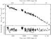 |
Fig. 6 X-ray light curve of the GRB 100621A afterglow with a broken power-law fit, ignoring the enhanced emission at 5−8 ks which we assign to the jump component (see Sect. 4.2.2). The decay slope from around 1 ks nicely continues until 80 ks, when it steepens to α = 1.54 ± 0.06. |
The overall shape of the rise, short shallow decay and subsequent fast decay is very similar to the behaviour of the afterglow of GRB 081029 (Nardini et al. 2011), where an analogous behaviour has been associated with the intrinsic properties of the GRB and not to changes in the intervening dust content. In the meantime, but independent of these observations, Vlasis et al. (2011) expanded the kinetic energy dominated energy injection scenario from Zhang & Meszaros (2002) and presented numerical simulations of the collision of an ultra-relativistic shell in a constant density environment with the external forward shock, which produce similar flare light curves. Figure 5 shows their case 4 model (with 2° half-opening angle; from their Fig. 7) plotted over the GROND J-band light curve. In this scenario, the fast rise occurs when a second shell reaches the back of the first, self-similar Blandford-McKee shell. The steepness and amplitude of the rise depend on the half-opening angle of the jet, the Lorentz factor of the two colliding shells, and most likely more parameters such as the energy, the occurrence time relative to the jet break, and ϵB. A much more extensive parameter study than that in Vlasis et al. (2011) is needed to be able to derive some of these parameters (or ranges thereof) for GRB 100621A. However, a qualitative conclusion would most likely be that GRB 100621A has a large Lorentz factor or a small half-opening angle, or both. Among the sample of a handful of GRBs showing such features (Greiner 2011), GRB 100621A shows the steepest rise in time: a formal fit with To at the GRB trigger results in αrise = 14 (which, because of its late appearance, is also insensitive to any possible change in To of the fit).
According to Vlasis et al. (2011), the rather flat part after the jump is then due to the merging of the two shells, the heating of which compensates the fading flux from the forward shock of the first shell. After the jump, the light curves should follow the predicted slopes for the normal, single forward shock, but at a higher intensity level because of the additional energy injection by the colliding second shell. While this is difficult to test convincingly with our data since the normal decay is not constrained accurately enough, the rise and the observed structure in the flat part of the light curve is surprisingly similar to the modelling in Vlasis et al. (2011), particularly their Fig. 6. We defer a more detailed comparison of this behaviour in GRB 100621A with this shell-collision model to a future paper.
 |
Fig. 7 Visualization of the spectral energy distributions at the five epochs as discussed in the text, with panel 1 to 3 showing epochs 1−3, panel 4 showing epochs 4 and 5, and panel 5 showing epochs 6 and 7. The frequency/energy ranges covered by our observations are marked as shaded bands. Dashed lines mark the different emission components: afterglow (blue), flares (green), jump component (red). The thick line is the sum of these components. |
4.2.3. The light curve beyond 20 ks
We have shown in Sect. 4.2.1 that the normal afterglow decay slope in the optical/NIR at a few ks after the GRB was αO = 0.69 ± 0.06. An extrapolation of this decay at the same decay rate, i.e. with continued energy injection at the same temporal rate, underpredicts the later GROND data by at least a factor of 2. Thus, the rate of energy injection would have had to increase over the early rate, if it were to explain the optical/NIR emission at To+20 ks. We consider this unlikely, and thus conclude that at late times, i.e. t > To + 20 ks, the optical/NIR fluxes are dominated by the process which led to the huge intensity jump at 4 ks. As the spectral shape of this emission was redder than that of the canonical afterglow, this statement will also be true for the sub-mm and radio bands (see next section). At X-rays, we have shown in the previous section that the contribution of the large intensity jump was marginal, at most 50%, during the peak emission of the intensity jump. If the X-ray emission associated to the jump component subsequently dropped the same way as the optical emission, then it faded by a factor of 20 in the interval from To+10 ks to To+30 ks. The total X-ray emission faded by just a factor of 2, implying that the X-ray emission beyond about To+10 ks can be solely attributed to the normal afterglow.
The fit to the X-ray light curve using a broken power law and ignoring the enhanced emission at 5−8 ks describes the overall behaviour very well. The break time is derived to be 80 ks, at which point the decay steepens to α = 1.54 ± 0.06 (Fig. 6).
This steepening of the light curve could be due to the cessation of the energy injection. However, for our value of β, a full cessation should lead to the canonical decay slopes of α = 1.72 (wind) or α = 1.22 (ISM) in the standard afterglow scenario, or α = 1.96 or steeper for any jet model (see below). Thus, only a partial cessation of energy injection would be a viable solution. Alternatively, the steepening could be due to the passage of the cooling break at continued energy injection. This would not work for the standard afterglow scenario of a spherical afterglow (i.e. Γ > 1/θ, where θ is the jet half-opening angle), since the predicted slope change is just Δα = 0.25. However, the predicted change is larger for a jetted outflow. Following Panaitescu et al. (2006), we consider two options, (i) a jet whose edge is visible and which does not expand laterally, and (ii) a jet with sharp edges which spreads laterally and is observed when Γ × θ < 1. In their Eqs. (34) and (35), Panaitescu et al. (2006) provide the flattening of light curves due to energy injection for the frequency range above and below νc. For option (i), the slopes depend on the circumburst medium density profile. Thus, we have three cases, each with a separate closure relation above and below νc. We start with the three cases for ν < νc and determine e, the power of the energy injection (see above) such that the observed early decay slope of α = 0.72 is reproduced (we choose to take the value consistent with both our measured αO and αX, though this would not change our upcoming conclusion). With each of the three different values of e, we then check the predicted slope at ν > νc for each of the three cases. Option (i) in the constant density environment returns the steepest slope, with αpred = 1.2 (for e = 0.75). This is still flatter than the observed αX = 1.54 ± 0.06 (Fig. 6). The predicted slope depends only very weakly on β, so also the trend of steepening βX towards the end of the observed X-ray light curve will not lead to consistency. We note that in this interpretation the energy injection is still active at the end of the X-ray light curve, i.e. at 2 × 10⁶ s, as we see no further steepening to a slope of α > 2.2 (depending on any further softening of βX).
Last, but not least, we note the coincidence of the measured slope of α = 1.54 ± 0.06 and the predicted αX = 1.48 for the decay of the ν > νc part of the afterglow in the spherical case. Thus, the steepening of the X-ray light curve at 80 ks could be due to the combination of both cessation of energy injection and passage of the cooling break in an ISM environment for an afterglow which is still in its spherical expansion phase (i.e. Γ > 1/θ) when the collimation is not yet detectable. Admittedly, the need for this coincidence is not an attractive solution. At the moment, we do not have a more satisfactory explanation for the amount of the steepening of X-ray light curve at To + 80 ks. However, a break of this kind in the X-ray light curve is very common in the sample of ≈700 Swift GRB afterglows, and so is a more generic problem (Nousek et al. 2006) rather than a problem related to the specifics of GRB 100621A.
4.2.4. Epochs 4 and 5
The two APEX/LABOCA detections correspond to a flux decay according to ~t-0.5 which then must accelerate considerably in order to be compatible with the upper limit at epoch 6. In the standard fireball scenario, the maximum in the sub-mm light curve is associated with the passage of the injection frequency. Since the observed decay slope is still considerably flatter than the expected t3(1 − p)/4 for ν < νm, the injection frequency of the dominating component should be near the LABOCA observing frequency during epochs 4 and 5. This is compatible with our best-fit SEDs: for epoch 4, the extrapolation of the GROND optical/NIR SED almost exactly reproduces the APEX/LABOCA measurement, while for epoch 5 the optical/NIR flux (determined from an interpolation between two GROND measurements) has faded more rapidly than the sub-mm flux, resulting in a move of νm to lower frequencies. The speed of this frequency displacement between epoch 4 and 5 is measured as t− 1.15 ± 0.55, consistent with the fireball prediction of t− 3/2. The observed optical/NIR flux is about a factor of 2 above the extrapolation of the decay of the canonical afterglow, thus we assign this emission to the jump component. In contrast, as shown in the previous sub-section, the X-ray emission is due to the canonical afterglow component. Curiously, despite the steeper X-ray spectrum, a formal SED fit including the X-rays is possible because of the large gap between the optical and X-ray bands. Since the X-ray spectrum has a steeper slope than the optical/NIR/sub-mm at this time, the large range allowed for νc can accommodate this bright X-ray component.
Thus, with the two assumptions that (i) the contemporaneously measured X-ray emission is a separate emission component, and is therefore left out from fitting; and (ii) the long-wavelength portion is dominated by the jump component, we make a combined spectral fit of epochs 3−6, where only epoch 3 contains X-ray data. We fix β1 = 1/3 and Δβ = 0.5 between the GROND and the Swift/XRT band, and also fix the host extinction at the value of AV = 3.65 mag as derived from the fit of epoch 3. With the lower S/N ratio of the later GROND SEDs, the slope in the GROND range is largely dominated by epoch 3, with a best-fit value for the combined fit of β2 = 0.90 ± 0.04. The ATCA measurements then define the break energy νm as summarized in Table 4. We note that a fireball-compliant evolution of νm from these values extrapolated backwards in time does not conflict the limit on νm set by the NIR data at 5.5 ks (see dashed line labelled t− 3/2 in Fig. 10).
4.2.5. Epochs 6 and 7
For these two epochs, we have the radio fluxes at two frequencies from the ATCA measurements. As described earlier, they are compatible with the ν1/3 slope as expected for the segment between νsa and νm. At sub-mm, the APEX/LABOCA upper limit is well above this spectral component, and does not constrain the SED.
The more or less unchanged radio flux in epochs 6 and 7 (formal fit results in t-0.5, although the large error bars of epoch 7 also allow a slightly rising flux) implies that the injection frequency is in the range of a few GHz (near our radio data). This conclusion is supported by two other observational constraints, namely that the radio spectral slope is somewhat flatter than ν1/3, and that the radio flux must decline within the following 20 days in order to be compatible with the ATCA upper limits (see Table 3).
A combined fit of the radio and optical/NIR data results in a best-fit injection frequency of the order of 2 × 10¹² Hz, a factor 1000 larger than our estimate above, and also a factor of 10 larger than one would expect from the fireball-compliant evolution of the jump component. This suggests that the radio emission belongs to the canonical afterglow component, while the optical/NIR belongs to the jump component (as argued above). This picture is again consistent with a fireball-compliant prediction of the early evolution of νm, i.e. that νm is at frequencies shortward of the GROND NIR measurements at very early times (see the blue dashed line in Fig. 10).
4.3. Characterization of the three emission components
First, Table 5 summarizes the discussion from the above sections with respect to the three emission components, and not according to the epoch of observation, and Fig. 7 provides a visualization of the evolution of these three components with time.
Epochs at which the three emission components are seen at different frequency bands.
With these constraints on the varying combination of the three emission components at a given epoch, the combined fitting results in a total reduced  (162 for 145 degrees of freedom), and so is an acceptable fit. The best fit power-law slope in the GROND range for the canonical afterglow (fully described in Sect. 4.2.1) is β2 = 0.82 ± 0.02 with a strong host extinction of AV = 3.65 ± 0.06 mag, as already indicated by the very red colours of the afterglow.
With the generic picture that the typical afterglow spectrum evolves from fast to slow cooling, we will now use the constraints for each of the components, and try to infer a consistent picture of the evolution of the GRB 100621A afterglow. The discussion is based on the formalism described in Granot & Sari (2002), and we use the same nomenclature of E52 = E/1052 erg, and  .
.
4.3.1. The canonical afterglow
The SED of epoch 1 provides four constraints on the fireball parameters of the canonical afterglow: (i) a lower limit on the frequency of νc at that time (>8 keV); (ii) an upper limit on the flux density at νc (<0.035 mJy); (iii) an upper limit on νm based on the non-detection of νm (or a break in general) in the GROND range, i.e. νm < 1.25 × 10¹⁴ Hz (<2.4 μm); and (iv) a lower limit on the flux at this limit frequency (>9 mJy). Using the two equations each in lines 3 and 5 of Table 2 of Granot & Sari (2002), these measurements translate into the four conditions ![Mathematical equation: \begin{equation} \begin{array}{l} {\rm ~~(i)} \hspace{1.cm} \epsilon_B^{-3/2} \cdot n^{-1} \cdot E_{52}^{-1/2} > 2.82\times10^4, \\[1mm] {\rm ~(ii)}\hspace{1.cm} \epse^{1.62} \cdot \epsilon_B^{2.12} \cdot n^{1.31} \cdot E_{52}^{1.81} < 7.17\times10^{-9}, \\[1mm] {\rm (iii)} \hspace{1.cm} \epse^2 \cdot \epsilon_B^{1/2} \cdot E_{52}^{1/2} < 6.46\times10^{-6}, \\[1mm] {\rm (iv)} \hspace{1.cm} \epsilon_B^{1/2} \cdot n^{1/2} \cdot E_{52} > 0.195. \\ \end{array} \end{equation}](/articles/aa/full_html/2013/12/aa21284-13/aa21284-13-eq196.png) (1)These equations define an upper limit on
(1)These equations define an upper limit on  (which translates into ϵe < 0.16 for our p = 2.64), and combined lower limits for ϵB and the external density as shown by the lines of arrows in Fig. 8.
 |
Fig. 8 Constraints on the microphysical parameters of the canonical afterglow component from the SED of epoch 1 at 520 s after the GRB (black triangles), and of epoch 6 (coloured arrows/lines). The limits on F(νm) and νc from epoch 1 allow the parameter space above the lines of open triangles (left panel), and an upper limit of |


In principle, there are two more constraints, namely the limit that the time of νm crossing νc (5 → 1 in Granot & Sari 2002) has occured within <520 s, and the transition 1 → 2 (νm crossing νsa) is constrained to >416 ks. However, these limits do not impose any additional constraints as shown in Fig. 8.
Epoch 3 does not provide any further constraint on the canonical afterglow, as the X-ray flux and spectral shape cannot be independently differentiated from that of the jump component, as mentioned above.
At epochs 4 and 5, the X-rays provide the only measurements of the canonical afterglow. Given the somewhat contrived conclusion that the late X-ray light curve after the break at 80 ks is due to a combination of cessation of energy injection and cooling break passage, and that it is still in the spherical phase, we refrain from adding these constraints here.
Epochs 6 and 7, after re-fitting without the GROND optical/NIR data, provide no unambiguous measurement of νm and F(νm) (or νc), because the normalization of the power-law segment that connects the ν− 1/3 segment with the X-ray segment is not constrained. Stepping through νm in the range 1 × 10⁻⁷ keV to 6 × 10⁻⁵ keV reveals equally good fits as long as νm > 5 × 10⁻⁶ keV (250 μm). With this limit we obtain ![Mathematical equation: \begin{equation} \begin{array}{l} {\rm ~~(i)} \hspace{1.cm} \epse^2 \cdot \epsilon_B^{1/2} \cdot E_{52}^{1/2} > 1.1\times10^{-3}, \\[1mm] {\rm ~(ii)} \hspace{1.cm} \epsilon_B^{1/2} \cdot n^{1/2} \cdot E_{52} < 0.017. \\ \end{array} \end{equation}](/articles/aa/full_html/2013/12/aa21284-13/aa21284-13-eq210.png) (2)All combined constraints for the afterglow component are shown in Fig. 8.
(2)All combined constraints for the afterglow component are shown in Fig. 8.
4.3.2. The early flares
The flares are only observed at early times, and for a description we have picked epoch 2 to cover some of them. While we called these events flares, it seems obvious that they are somewhat dissimilar to the canonical X-ray flares observed by Swift/XRT in a large fraction of GRBs. In the case of GRB 100621A, the flares are prominent in the optical, rather than in X-rays. If these have the same origin as the canonical X-ray flares (Margutti et al. 2011), the only difference might be a lower peak energy. The broad-band spectrum between GROND and Swift/XRT is certainly not a single power law (see Sect. 4.2.1). As the low-energy part of a broken power-law fit (β = 0.86) would be very steep for a Band function approach, the peak energy Epeak is instead below the GROND wavelengths, with possibly some exponential cut-off at X-rays. Since the decomposition into the normal afterglow component and the flare component is not unique, no statement can be made on a possible variation of the peak energy with time.
4.3.3. The jump component
As mentioned earlier, the Vlasis et al. (2011) interpretation of the optical/NIR emission at 5−8 ks is via the collision of two ultrarelativistic shells. The SED of the 5−8 ks event exhibits a straight power law of slope 1.1 ± 0.1 covering the GROND optical/NIR and the Swift/XRT region. If interpreted using the Granot & Sari (2002) formalism for afterglows (the applicability of which is not obvious because the medium into which the colliding shell is evolving might be increasing in density, rather than being constant or decreasing), the location of νc and νm remain ambiguous. If νc were longwards of 2.4 μm (GROND Ks-band), then the electron spectral index would be a reasonable p = 2.2. However, in addition to the observed light curve decay at >10 ks being much steeper than the expected t-1.15, there would be further inconsistencies: (1) if the circumburst environment had a wind density profile, νc would evolve to higher frequencies, i.e. into the GROND band, which is not observed; (2) if, alternatively, the circumburst density profile were ISM-like, νc would move towards the LABOCA band. However, at epoch 4 the optical/NIR SED extrapolates almost perfectly to the measured LABOCA flux, thereby not allowing any break. Thus, νc would have to be below 345 GHz at epoch 3. This would imply a later radio flux at least a factor of 103 larger than observed, and therefore can be excluded. We thus conclude that νc at epoch 3 must be >8 keV, implying a steep p = 3.2. Using these constraints, we arrive at the four conditions ![Mathematical equation: \begin{equation} \begin{array}{l} {\rm ~~(i)} \hspace{1.cm} \epsilon_B^{-3/2} \cdot n^{-1} \cdot E_{52}^{-1/2} > 1.58\times10^5, \\[2mm] {\rm ~(ii)}\hspace{1.cm} \epse^{2.2} \cdot \epsilon_B^{-1/2} \cdot n^{1.6} \cdot E_{52}^{2.1} < 2.47\times10^{-10}, \\[2mm] {\rm (iii)} \hspace{1.cm} \epse^2 \cdot \epsilon_B^{1/2} \cdot E_{52}^{1/2} < 2.36\times10^{-4}, \\[2mm] {\rm (iv)} \hspace{1.cm} \epsilon_B^{1/2} \cdot n^{1/2} \cdot E_{52} > 0.358. \\ \end{array} \end{equation}](/articles/aa/full_html/2013/12/aa21284-13/aa21284-13-eq218.png) (3)None of these conditions is violated by the constraints derived below for the emission of the 5−8 ks event.
(3)None of these conditions is violated by the constraints derived below for the emission of the 5−8 ks event.
The SED of this 5−8 ks event is constrained by our measurements of epochs 4 and 5 and 6 and 7. During epoch 4, we measure νm and F(νm), which provides the two equations ![Mathematical equation: \begin{equation} \begin{array}{l} {\rm ~~(i)} \hspace{1.cm} \epse^2 \cdot \epsilon_B^{1/2} \cdot E_{52}^{1/2} = 7.0\times10^{-5}, \\[2mm] {\rm ~(ii)} \hspace{1.cm} \epsilon_B^{1/2} \cdot n^{1/2} \cdot E_{52} = 0.716. \\ \end{array} \end{equation}](/articles/aa/full_html/2013/12/aa21284-13/aa21284-13-eq219.png) (4)Epochs 6 and 7 provide an interesting constraint on the sub-mm/radio regime, despite the non-detections longward of the GROND-K band. The APEX/LABOCA non-detection does not constrain the continuation of the optical/NIR slope into the mm-band, but a fireball-compliant extrapolation would suggest νm ≈ 1 × 10¹¹ Hz at epoch 6. Since we have argued earlier that the radio emission seen at this epoch at 5.5 and 9 GHz must belong to the canonical afterglow, we have to assume that the radio-component of the jump component must be self-absorbed to a level to not exceed the measured fluxes at 5.5 and 9 GHz. This results in νsa 0.8 × 10¹¹ Hz, i.e. νm = νsa at epoch 6 and 7 to within the errors. This is exactly what Vlasis et al. (2011) find during the modelling of the radio light curve: the amplitude is strongly depressed because of self-absorption.
(4)Epochs 6 and 7 provide an interesting constraint on the sub-mm/radio regime, despite the non-detections longward of the GROND-K band. The APEX/LABOCA non-detection does not constrain the continuation of the optical/NIR slope into the mm-band, but a fireball-compliant extrapolation would suggest νm ≈ 1 × 10¹¹ Hz at epoch 6. Since we have argued earlier that the radio emission seen at this epoch at 5.5 and 9 GHz must belong to the canonical afterglow, we have to assume that the radio-component of the jump component must be self-absorbed to a level to not exceed the measured fluxes at 5.5 and 9 GHz. This results in νsa 0.8 × 10¹¹ Hz, i.e. νm = νsa at epoch 6 and 7 to within the errors. This is exactly what Vlasis et al. (2011) find during the modelling of the radio light curve: the amplitude is strongly depressed because of self-absorption.
 |
Fig. 9 Constraints on the microphysical parameters of the jump component, derived from epochs 4 and 5 and 6 and 7 (see text) for the case of a constant ISM density profile. |
In a constant external density profile, νsa is constant, and our above assumption does not violate any observational constraint at earlier or later times. For a wind environment, νsa decreases according to t− 3/5; this is slow enough that it does not conflict with the LABOCA detections at epochs 4 and 5.
Thus, for the ISM case, we derive ![Mathematical equation: \begin{equation} \begin{array}{l} {\rm (iii)} \hspace{1.cm} \epse~^{-1} \cdot \epsilon_B^{1/5} \cdot n^{3/5} \cdot E_{52}^{1/5} = 538, \\[2mm] {\rm (iv)} \hspace{1.cm} \epse~^{-1} \cdot \epsilon_B^{2/5} \cdot n^{7/10} \cdot E_{52}^{9/10} > 123. \\ \end{array} \end{equation}](/articles/aa/full_html/2013/12/aa21284-13/aa21284-13-eq225.png) (5)The combination of the last four equations translates into the two thin stripes of parameter space shown in Fig. 9. The resulting limits on the external density are rather high: since ϵB cannot be larger than 1, the external density must be 20 cm-3. Moreover, the total energy is constrained to E52 > 0.2, and
(5)The combination of the last four equations translates into the two thin stripes of parameter space shown in Fig. 9. The resulting limits on the external density are rather high: since ϵB cannot be larger than 1, the external density must be 20 cm-3. Moreover, the total energy is constrained to E52 > 0.2, and  . We stress again that these constraints are only valid if the Granot & Sari (2002) formalism is applicable.
5. Discussion
5.1. Fitting assumptions and results
The behaviour of the afterglow of GRB 100621A at different epochs and frequencies has been found to be too complex compared to our set of observational data to be able to constrain models. We have therefore adopted the fireball scenario and attempted to construct a consistent picture of the observed features. Before further discussion, we summarize our assumptions here: (i) we assume that the total emission is due to the superposition of three emission components; (ii) we have fixed Δβ = 0.5 between X-ray and GROND power-law slopes (whenever applicable); (iii) we have fixed βradio = −1/3 as derived from the two radio frequencies at epochs 6 and 7; and (iv) we had to assume that the the jump component has to be self-absorbed in the radio. With these assumptions, we find a reasonably consistent picture which describes all of our observational facts (temporal and spectral slopes) except the slow X-ray decay at times >80 ks.
For none of the three emission components in the afterglow of GRB 100621A do we have enough observations at the right time to determine all fireball model parameters in a unique way. The constraints on these parameters derived from our observations are, in general, broadly consistent with expectations. The only inconsistent result is for ϵB of the afterglow component: the lower limits from epoch 1 are about 2 orders of magnitude higher than the upper limits derived from epochs 6 and 7, assuming otherwise equal parameters (in particular total energy and density). There could be several reasons for this, an evolving ϵB with time for example, though we do not consider this. A more obvious reason could be that the energy ejection (which was deduced to make spectral and temporal slopes in the early phases consistent with the fireball scenario) introduces a time-dependent variation between low- and high-frequency segments (at radio wavelength the impact of the energy injection will come later than at X-rays). This invalidates our assumption for epochs 6 and 7 in deriving constraints on νm, in that the radio and X-ray sections of the SED reflect the same internal energy budget. We therefore neglect the νm constraints from epochs 6 and 7 in the following. If we allow νm to be just above 9 GHz during epochs 6 and 7, then conflicting constraints are no longer imposed.
 |
Fig. 10 Location of the two breaks νc (top end) and νm (bottom part) at different epochs in the late-time evolution of the afterglow of GRB 100621A, for each of the three emission components (i) canonical afterglow (black); (ii) flares (red); and (iii) jump component (pink). Vertical bars indicate allowed ranges for νc or νm. The wavelength coverage of our instruments is shown as vertical bars at the very left side. Dashed lines show the expected evolution according to the standard fireball scenario after obeying the limits derived from our observations at various epochs. |
Despite the complex behaviour, we are able to unequivocally deduce a constant ISM-like circumburst density profile. The slow intensity decline of the external forward shock suggests continuous energy injection at a rate proportional to t0.35 during the first hour after the GRB. With the onset of the jump component, another sudden increase in energy happens which lifts the energy budget by a factor of 2−5.
One could imagine that the canonical afterglow and the early flares experience the same external ISM density, i.e. that they originate co-spatially. In this case, the combined constraints imply that the external density n 50 cm-3, otherwise the F(νm) limit for the afterglow component would be violated. This in turn would imply that the energy driving the flares would be of the order of Eiso (1 < E52 < 5), which is surprisingly large though not exceptional. Correspondingly, we deduce  and ϵB > 10-4.
For the jump component, as mentioned above, we derived n 20 cm-3. This is interesting as one could have imagined that this component originates in the wake of the afterglow, i.e. in a region cleared by the forward shock. However, we caution (again) that the interpretation with the Granot & Sari (2002) framework might not be appropriate at all. Further theoretical investigation of such shell collisions are certainly warranted.
5.2. Location of the dust
From multiple SED fits during the early rise and early plateau (around 200−400 s after the GRB trigger) we constrain any variation of the extinction to ΔAV < 10%. It has been repeatedly suggested that the intense radiation of gamma-ray bursts destroys the dust in its near environment through sublimation (Waxman & Draine 2000; Fruchter et al. 2001; Perna & Lazzati 2002) out to distances of a dozen parsec. The large dust column we observe in the afterglow of GRB 100621A must therefore be at larger distances, most likely not related to the star formation site of the progenitor of GRB 100621A.
 |
Fig. 11 Comparison of our GRB 100621A sub-mm light curve to previous sub-mm observations of GRBs with more than one observation, and selected upper limits for a few famous GRBs. Different symbols mark different observer frequencies, and colours denote different GRBs (except for the upper limits). Data are from GRB 030329: Kohno et al. (2005); Sheth et al. (2003); GRB 090313: Greiner et al. (in prep.); GRB 080129: Greiner et al. (2009b); GRB 090423: Bock et al. (2009); GRBs 091102, 110709B, 110715A, 100901A, and 110918A: de Ugarte Postigo et al. (2012). |
5.3. Comparison with previous sub-mm detections
Previous sub-mm measurements of GRB afterglows were initially non-detections (Bremer et al. 1998; Shephard et al. 1998), and detections or even light curves are sparse (Chandra et al. 2008; Sheth et al. 2003; Greiner et al. 2009b; Perley et al. 2012; Zauderer et al. 2012). Predictions of emission at flux levels of several tens of mJy (e.g. Inoue et al. 2005) have not materialized. So far, only a handful of GRBs have been detected in the mm/sub-mm, mostly using MAMBO at the IRAM 30 m (Chandra et al. 2008; Sheth et al. 2003; Greiner et al. 2009b), and CARMA (Chandra et al. 2007; Bock et al. 2009; Perley et al. 2012). GRB 100621A is one of a handful of GRBs for which a sub-mm light curve (more than one detection) is available (Fig. 11). However, the complicated early optical/NIR light curve of GRB 100621A makes even this relatively well-observed GRB too sparsely sampled in the sub-mm range, which leaves ambiguities in the interpretation of both, the light curve and the movement of the low-frequency break.
Recent more aggressive attempts with APEX/LABOCA have continued to return mostly non-detections (de Ugarte Postigo et al. 2012), indicating that the injection frequency moves rather rapidly to frequencies below the LABOCA range, thus requiring sub-mm observations within the first day in order to achieve detections. APEX/LABOCA is able to do this for the best suited afterglows (steep optical/NIR SED), but for the majority ALMA will be the instrument of choice, once rapid turn-around target-of-opportunity observations are offered.
5.4. The GRB host
The host galaxy of GRB 100621A was extensively covered in Krühler et al. (2011b), including in addition to the GROND and Swift/UVOT data. In short, the r′ ≈ 21.5 mag galaxy is well detected from the UV (all Swift/UVOT filters) up to the Ks-band showing a very blue spectral energy distribution with (R − K)AB ≈ 0.3 mag. The stellar population synthesis fitting of the host SED returns an age of the dominating stellar population of only 0.05 Gyr, and an intrinsic extinction of  mag, in stark contrast to the large afterglow (AG) extinction of
  mag. The absolute magnitude of the host is MB = −20.68 ± 0.08 mag, and the star formation rate was determined as 13
 M⊙/yr.
The APEX and ATCA non-detections of any flux at the position of GRB 100621A at >5 days after the GRB also provide first crude limits on the sub-mm and radio emission of the host galaxy, of <6.8 mJy at 345 GHz, <170 μJy at 5.5 GHz, and <200 μJy at 9 GHz (all 2σ confidence). Assuming that the dominant fraction of the radio emission would be of non-thermal origin, and using the formalism of Yun & Carilli (2002), this implies an upper limit on the star formation rate of 100 M⊙/yr.
Because of the bright, compact host, no observational attempt has been made with GROND to search for the supernova component which would have peaked about 6 mag fainter (if extinguished the same way as the afterglow) than the host brightness for a 1998bw-like SN-luminosity.
6. Conclusions
The afterglow of GRB 100621A has shown the brightest X-ray emission of any gamma-ray burst so far. Despite this, the afterglow at 200 s was not extraordinarily bright, and the strong host extinction made it only marginally detectable in Swift/UVOT observations. Yet, we obtained a decent data set with GROND as well as supporting APEX/LABOCA and ATCA measurements.
The biggest surprise in the properties of the afterglow of GRB 100621A is undoubtly the sudden intensity jump after about 1 hr. Here, we have been able to characterize its properties in hitherto unprecedented detail. The peculiarity of this event is the complexity of the combined afterglow emission which we encounter. In order to disentangle this complexity, and to possibly even test afterglow models, a much denser sampling of the afterglow emission in time is required, both at sub-mm and radio frequencies. For sub-mm observations from the southern hemisphere, ALMA would be an ideal instrument if fast reaction times to external alerts like gamma-ray bursts can be implemented.
Throughout this paper we use the definition Fν ∝ t− αν− β where α is the temporal decay index, and β is the spectral slope.
APEX is a collaboration between the Max-Planck-Institut für Radioastronomie, the European Southern Observatory and the Onsala Space Observatory.
Acknowledgments
J.G. expresses special thanks to A. Vlasis for discussing some details of the shell collision scenario. We are grateful to ESO for approving the DDT proposal for APEX observations. Particular thanks to A. Kaufer for the support in the scheduling discussions for technical and Chilean time. A.M. was a fully sponsored Ph.D. candidate at ICRAR − Curtin University until 2011 and acknowledges the support of SHAO as a postdoctoral research fellow. We are similarly grateful to P. Edwards for approving and scheduling the ATCA ToO and regular observations. T.K. acknowledges support by the DFG cluster of excellence “Origin and Structure of the Universe” during the early part of this project when being employed at MPE, and AU is grateful for travel funding support through MPE. F.O.E. acknowledges funding of his Ph.D. through the Deutscher Akademischer Austausch-Dienst (DAAD), S.K. and A. Rossi acknowledge support by DFG grant Kl 766/13-2, and S.K., A. Rossi, A.N.G. and D.A.K. acknowledge support by DFG grant Kl 766/16-1. ARossi additionally acknowledges support from the BLANCEFLOR Boncompagni-Ludovisi, née Bildt foundation, and through the Jenaer Graduiertenakademie. M.N acknowledges support by DFG grant SA 2001/2-1. Part of the funding for GROND (both hardware and personnel) was generously granted from the Leibniz-Prize to Prof. G. Hasinger (DFG grant HA 1850/28-1). The Dark Cosmology Center (TK) is funded by the Danish National Research Foundation. This work made use of data supplied by the UK Swift Science Data Centre at the University of Leicester. Facilities: Max Planck:2.2 m (GROND), Swift
References
- Beuermann, K., Hessman, F. V., Reinsch, K., et al. 1999, A&A, 352, L26 [NASA ADS] [Google Scholar]
- Blustin, A. J., Band, D., Barthelmy, S., et al. 2006, ApJ, 637, 901 [NASA ADS] [CrossRef] [Google Scholar]
- Bock, D. C.-J., Chandra, P., Frail, D. A., & Kulkarni, S. R. 2009, GCN, #9274 [Google Scholar]
- Bremer, M., Krichbaum, T. P., Galama, T. J., et al. 1998, A&A, 332, L13 [NASA ADS] [Google Scholar]
- Chandra, P., Bock, D., Soderberg, A., et al. 2007, GCN, 6073 [Google Scholar]
- Chandra, P., Cenko, S. B., Frail, D. A., et al. 2008, ApJ, 683, 924 [NASA ADS] [CrossRef] [Google Scholar]
- de Ugarte Postigo, A., Lundgren, A., Martin, S., et al. 2012, A&A, 538, 44D [Google Scholar]
- Evans, P. A., Beardmore, A. P., Page, K. L., et al. 2007, A&A, 469, 379 [NASA ADS] [CrossRef] [EDP Sciences] [Google Scholar]
- Evans, P. A., Beardmore, A. P., Page, K. L., et al. 2009, MNRAS, 397, 1177 [NASA ADS] [CrossRef] [Google Scholar]
- Evans, P. A., Goad, M. R., Osborne, J. P., & Beardmore, A. P. 2010, GCN, #10873 [Google Scholar]
- Filgas, R., Greiner, J., Schady, P., et al. 2012, A&A, 535, A57 [Google Scholar]
- Fruchter, A., Krolik, J. H., & Rhoads, J. E. 2001, ApJ, 563, 597 [NASA ADS] [CrossRef] [Google Scholar]
- Gehrels, N., Chincarini, G., Giommi, P., et al. 2004, ApJ, 621, 558 [Google Scholar]
- Ghirlanda, G., Nava, L., Ghisellini, G., et al. 2012, MN, 420, 483 [Google Scholar]
- Golenetskii, S., Aptekar, R., Frederiks, D., et al. 2010, GCN, #10882 [Google Scholar]
- Granot, J., & Sari, R. 2002, ApJ, 568, 820 [NASA ADS] [CrossRef] [Google Scholar]
- Granot, J., Piran, T., & Sari, R. 1999, ApJ, 527, 236 [NASA ADS] [CrossRef] [Google Scholar]
- Greiner, J. 2011, talk at The prompt activity of Gamma-Ray Bursts, Rayleigh, March 2011, http://grb.physics.ncsu.edu/GRB_2011/WEB/TALKS/greiner.pdf [Google Scholar]
- Greiner, J., Bornemann, W., Clemens, C., et al. 2008, PASP, 120, 405 [NASA ADS] [CrossRef] [Google Scholar]
- Greiner, J., Krühler, T., Fynbo, J. P.U, et al. 2009a, ApJ, 693, 1610 [NASA ADS] [CrossRef] [Google Scholar]
- Greiner, J., Krühler, T., McBreen, S., et al. 2009b, ApJ, 693, 1912 [NASA ADS] [CrossRef] [Google Scholar]
- Greiner, J., Krühler, T., Klose, S., et al. 2011, A&A, 526, A30 [NASA ADS] [CrossRef] [EDP Sciences] [Google Scholar]
- Inoue, S., Omukai, K., Ciardi, B. 2005, MNRAS, 380, 1715 [NASA ADS] [CrossRef] [Google Scholar]
- Kohno, K., Tosaki, T., Okuda, T., et al. 2005, PASJ, 57, 147 [NASA ADS] [CrossRef] [Google Scholar]
- Kovács, A. 2008, Proc. SPIE, 7020, 70201S-15 [Google Scholar]
- Krühler, T., Küpcü Yoldaş, A.,Greiner, J., et al. 2008, ApJ, 685, 376 [NASA ADS] [CrossRef] [Google Scholar]
- Krühler, T., Schady, P., Greiner, J., et al. 2011a, A&A, 526, A153 [NASA ADS] [CrossRef] [EDP Sciences] [Google Scholar]
- Krühler, T., Greiner, J., Schady, P., et al. 2011b, A&A, 534, A108 [NASA ADS] [CrossRef] [EDP Sciences] [Google Scholar]
- Küpcü Yoldaş, A., Krühler, T., Greiner, J., et al. 2008, AIP, Conf. Proc., 1000, 227 [Google Scholar]
- Margutti, R., Bernardini, G., & Barniol Duran, R. 2011, MNRAS, 410, 1064 [NASA ADS] [CrossRef] [Google Scholar]
- Meszaros, P., & Rees, M. J. 1997, ApJ, 476, 232 [NASA ADS] [CrossRef] [Google Scholar]
- Mészáros, P., Rees, M. J., & Wijers, R. A. M. J. 1998, ApJ, 499, 301 [NASA ADS] [CrossRef] [Google Scholar]
- Milvang-Jensen, B., Goldoni, P., Tanvir, N. R., et al. 2010, GCN, #10876 [Google Scholar]
- Molinari, E., Vergani, S. D., Malesani, D., et al. 2007, A&A, 469, L13 [NASA ADS] [CrossRef] [EDP Sciences] [Google Scholar]
- Naito, H., Sako, T., Suzuki, D., et al. 2010, GCN, #10881 [Google Scholar]
- Nardini, M., Greiner, J., Krühler, T., et al. 2011, A&A, 531, A39 [NASA ADS] [CrossRef] [EDP Sciences] [Google Scholar]
- Nousek, J. A., Kouveliotou, C., Grupe, D., et al. 2006, ApJ, 642, 389 [NASA ADS] [CrossRef] [Google Scholar]
- Panaitescu, A., & Vestrand, W. T. 2008, MNRAS, 387, 497 [NASA ADS] [CrossRef] [Google Scholar]
- Panaitescu, A., Meszaros, P., Gehrels, N., et al. 2006, MNRAS, 366, 1357 [NASA ADS] [CrossRef] [Google Scholar]
- Pandey, S. B., Rujopakarn, W., Guver, T., et al. 2010, GCN, #10871 [Google Scholar]
- Pei, Y. C. 1992, ApJ, 395, 130 [NASA ADS] [CrossRef] [Google Scholar]
- Perley, D. A., Alatalo, K., & Horesh, A. 2012, GCN, 13175 [Google Scholar]
- Perna, R., & Lazzati, D. 2002, ApJ, 580, 261 [NASA ADS] [CrossRef] [Google Scholar]
- Racusin, J. L., Karpov, S. V., Sokolowski, M., et al. 2008, Nature, 455, 183 [Google Scholar]
- Sari, R. 1999, ApJ, 524, L43 [NASA ADS] [CrossRef] [Google Scholar]
- Sari, R., Piran, T., & Narayan, R. 1998, ApJ, 497, L17 [NASA ADS] [CrossRef] [Google Scholar]
- Schlegel, D., Finkbeiner, D., & Davis, M. 1998, ApJ, 500, 525 [NASA ADS] [CrossRef] [Google Scholar]
- Schuller, F. 2012, Proc. SPIE, 8452, id. 84521T-10 [Google Scholar]
- Shepherd, D. S., Frail, D. A., Kulkarni, S. R., & Metzger, M. R. 1998, ApJ, 497, 859 [NASA ADS] [CrossRef] [Google Scholar]
- Sheth, K., Frail, D. A., White, S., et al. 2003, ApJ, 595, 33 [Google Scholar]
- Siringo, G., Kreysa, E., Kovacs, A., et al. 2009, A&A 497, 945 [Google Scholar]
- Skrutskie, M. F., Cutri, R. M., Stiening, R., et al. 2006, AJ 131, 1163 [Google Scholar]
- Tody, D. 1993, in Astronomical Data Analysis Software and Systems II, eds. R. J. Hanisch, R. J. V. Brissenden, & J. Barnes, ASP, Conf., 52, 173 [Google Scholar]
- Ukwatta, T. N., Barthelmy, S. D., Baumgartner, W. H., et al. 2010a, GCN #10870 [Google Scholar]
- Ukwatta, T. N., Stratta, G., Evans, P. A., et al. 2010b, GCN report 191.1 [Google Scholar]
- Updike, A., Nicuesa Guelbentu, A., Nardini, M., Krühler, T., & Greiner, J. 2010, GCN #10874 [Google Scholar]
- Vlasis, A., van Eerten, H. J., Meliani, Z., & Keppens, R. 2011, MNRAS, 415, 279 [NASA ADS] [CrossRef] [Google Scholar]
- Waxman, E., & Draine, B. T. 2000, ApJ, 537, 796 [NASA ADS] [CrossRef] [Google Scholar]
- Wijers, R. A. M. J., & Galama, T. 1999, ApJ, 523, 177 [NASA ADS] [CrossRef] [Google Scholar]
- Wijers, R. A. M. J., Rees, M. J., Meszaros, P., et al. 1997, MN 288, L51 [Google Scholar]
- Yun, M. S., & Carilli, C. L. 2002, ApJ, 568, 88 [NASA ADS] [CrossRef] [Google Scholar]
- Zauderer, B., Laskar, T., & Berger, E. 2012, GCN, 13900 [Google Scholar]
- Zhang, B., & Mészáros, P. 2002, ApJ, 566, 712 [NASA ADS] [CrossRef] [Google Scholar]
All Tables
Epochs at which the three emission components are seen at different frequency bands.
All Figures
|
Fig. 1 GROND i′-band finding chart of GRB 100621A, including the photometric comparison stars (roman and arabic letters). North is up, and east to the left. |
| In the text | |
|
Fig. 2 Afterglow light curve of GRB 100621A as observed with Swift in X-rays (top) and GROND in its seven filter bands (bottom). The J-band data points at 14 ks are from SOFI imaging, and the HKs-band data at 20 ks from a GROND observation in morning twilight at which the J-band was already saturated by the rising Sun. The seven vertical lines mark the times at which spectral energy distributions have been extracted (see text and Fig. 3). |
| In the text | |
|
Fig. 3 Multi-epoch SEDs (different colours) of the late-time afterglow of GRB 100621A as measured by Swift/XRT (right; not NH-corrected), GROND (middle; not AV-corrected)), APEX/LABOCA (middle left), and ATCA (far left), together with a broad-band model which fits all data available for the given epoch. The times of these SEDs are marked with vertical lines in Fig. 2, and the resulting break energies given in Table 4. Since the optical/NIR and X-ray fluxes in epochs 1−3 are very similar, epoch 3 (jump component at 6.8 ks) has been scaled upwards by a factor of 20, and epoch 2 (flares) down-scaled by a factor of 4. The curvature in the GROND data is due to strong extinction of the afterglow light in the host galaxy (dotted line). The breaks seemingly show erratic variations in frequency – see text for an interpretation. We do not consider the fits in this plot to be the final physical interpretation of the data, as it links emission components at different wavelength regions that do not belong together (see text). |
| In the text | |
|
Fig. 4 (Top panel) Comparison of the fluxed X-ray light curve at 10 keV; (middle panel) the GROND J (yellow), H (blue), Ks (green) bands; (bottom panel) the photon index of the X-ray spectrum (black, left y-axis scale) and the residuals of the model fit (see text) to the GROND JHK data (colour as in the middle panel, right y-axis scale). The diagonal-hatched region denotes epoch 1, the cross-hatched regions epoch 2. The dashed vertical lines mark the maxima in the photon spectral index Γ (Γ = β + 1) to guide the eyes. |
| In the text | |
|
Fig. 5 Early part of the GROND J-band light curve with a (slightly stretched in time) model of the two-shell collisions overplotted (case 4, Fig. 7 in Vlasis et al. 2011). Though this model was not aimed at reproducing the behaviour of the GRB 100621A afterglow, the similarity of the rise, structure at the peak, and the decay slope is striking. The early part of the model should be ignored, as it depends on the relative timing of the forward shock of the first shell, the ISM density, and the initial Lorentz factor. |
| In the text | |
|
Fig. 6 X-ray light curve of the GRB 100621A afterglow with a broken power-law fit, ignoring the enhanced emission at 5−8 ks which we assign to the jump component (see Sect. 4.2.2). The decay slope from around 1 ks nicely continues until 80 ks, when it steepens to α = 1.54 ± 0.06. |
| In the text | |
|
Fig. 7 Visualization of the spectral energy distributions at the five epochs as discussed in the text, with panel 1 to 3 showing epochs 1−3, panel 4 showing epochs 4 and 5, and panel 5 showing epochs 6 and 7. The frequency/energy ranges covered by our observations are marked as shaded bands. Dashed lines mark the different emission components: afterglow (blue), flares (green), jump component (red). The thick line is the sum of these components. |
| In the text | |
|
Fig. 8 Constraints on the microphysical parameters of the canonical afterglow component from the SED of epoch 1 at 520 s after the GRB (black triangles), and of epoch 6 (coloured arrows/lines). The limits on F(νm) and νc from epoch 1 allow the parameter space above the lines of open triangles (left panel), and an upper limit of |
| In the text | |
|
Fig. 9 Constraints on the microphysical parameters of the jump component, derived from epochs 4 and 5 and 6 and 7 (see text) for the case of a constant ISM density profile. |
| In the text | |
|
Fig. 10 Location of the two breaks νc (top end) and νm (bottom part) at different epochs in the late-time evolution of the afterglow of GRB 100621A, for each of the three emission components (i) canonical afterglow (black); (ii) flares (red); and (iii) jump component (pink). Vertical bars indicate allowed ranges for νc or νm. The wavelength coverage of our instruments is shown as vertical bars at the very left side. Dashed lines show the expected evolution according to the standard fireball scenario after obeying the limits derived from our observations at various epochs. |
| In the text | |
|
Fig. 11 Comparison of our GRB 100621A sub-mm light curve to previous sub-mm observations of GRBs with more than one observation, and selected upper limits for a few famous GRBs. Different symbols mark different observer frequencies, and colours denote different GRBs (except for the upper limits). Data are from GRB 030329: Kohno et al. (2005); Sheth et al. (2003); GRB 090313: Greiner et al. (in prep.); GRB 080129: Greiner et al. (2009b); GRB 090423: Bock et al. (2009); GRBs 091102, 110709B, 110715A, 100901A, and 110918A: de Ugarte Postigo et al. (2012). |
| In the text | |
Current usage metrics show cumulative count of Article Views (full-text article views including HTML views, PDF and ePub downloads, according to the available data) and Abstracts Views on Vision4Press platform.
Data correspond to usage on the plateform after 2015. The current usage metrics is available 48-96 hours after online publication and is updated daily on week days.
Initial download of the metrics may take a while.