| Issue |
A&A
Volume 559, November 2013
|
|
|---|---|---|
| Article Number | A131 | |
| Number of page(s) | 7 | |
| Section | Interstellar and circumstellar matter | |
| DOI | https://doi.org/10.1051/0004-6361/201322562 | |
| Published online | 27 November 2013 | |
The au-scale structure in diffuse molecular gas towards ζ Persei⋆
1 Institut d’Astrophysique de Paris (IAP), UMR7095 CNRS, Université Pierre et Marie Curie – Paris 6, 98bis boulevard Arago, 75014 Paris, France
e-mail: This email address is being protected from spambots. You need JavaScript enabled to view it.
2 Department of Physics and Astronomy, University of Toledo, Toledo, OH 43606, USA
3 Institut d’Astrophysique Spatiale (IAS), UMR 8617, CNRS, Bâtiment 121, Université Paris Sud 11, 91405 Orsay, France
4 LERMA (UMR 8112 du CNRS), Observatoire de Paris, 61 Avenue de l’Observatoire, 75014 Paris, France
5 Department of Astronomy, University of Washington, Seattle, WA 98195, USA
Received: 29 August 2013
Accepted: 9 October 2013
Abstract
Context. Spatial structure in molecular material has a strong impact on its physical and chemical evolution and is still poorly known, especially on very small scales.
Aims. To better characterize the small-scale structure in diffuse molecular gas and in particular to investigate the CH+ production mechanism, we study the spatial distribution of CH+, CH, and CN towards the bright star ζ Per on scales in the range 1−20 AU.
Methods. We use ζ Per’s proper motion and the implied drift of the line of sight through the foreground gas at a rate of about 2 AU yr-1 to probe absorption line variations between adjacent lines of sight. The good S/N, high or intermediate resolution spectra of ζ Per, obtained in the interval 2003−2011, allow us to search for low column-density and line width variations for CH+, CH, and CN.
Results. CH and CN lines appear remarkably stable in time, implying an upper limit δN/N ≤ 6% for CH and CN (3σ limit). The weak CH+λ4232 line shows a possible increase of 11% during the interval 2004−2007, which appears to be correlated with a comparable increase in the CH+ velocity dispersion over the same period.
Conclusions. The excellent stability of CH and CN lines implies that these species are distributed uniformly to good accuracy within the cloud. The small size implied for the regions associated with the CH+ excess is consistent with scenarios in which this species is produced in very small (a few AU) localized active regions, possibly weakly magnetized shocks or turbulent vortices.
Key words: astrochemistry / ISM: structure / ISM: molecules
Based on observations made at McDonald Observatory (USA) and Observatoire de Haute-Provence (France).
© ESO, 2013
1. Introduction
The presence of small-scale structure within interstellar material, together with its strong potential impact on the physical and chemical evolution of the gas, is now recognized. Many studies have been devoted to the distribution of H i in the atomic phase (see, e.g., Roy et al. 2012 and references therein) or to tracers such as Na i, K i, and Ca ii (Welty et al. 2008; Crawford 2003, Smith et al. 2013). On the other hand, the data concerning diffuse molecular gas remains relatively limited (Moore & Marscher 1995; Pan et al. 2001; Falgarone et al. 2009; Boissé et al. 2009; Cordiner et al. 2013), while this phase is of prime interest. Evidence of high pressure fluctuations is also provided by Jenkins & Tripp (2011) using C i, a good tracer of diffuse molecular gas. The small-scale distribution of CH+ in particular could provide useful clues to the longstanding “CH+ formation problem”. Indeed, the main scenarios proposed so far for overcoming the large energy barrier (4640 K) in the formation reaction of this species (C+ + H2 → CH+ + H) – shocks and vortices – both imply the existence of small-scale structure.
A few years ago, in order to complement the limited data available on the small-scale structure of molecules, we undertook a follow-up of several absorption lines from H2, CH, and CH+ towards the runaway star AE Aur (or HD 34078). We used the rapid motion of this O star to sample a broad range of scales in the foreground gas within a limited time interval. However, FUSE observations revealed an unexpected large amount of highly excited H2, which indicated that the intervening gas is most likely located very close to the star and strongly interacting with it (Boissé et al. 2005). Then, the time variations seen for CH and CH+ absorption lines (Boissé et al. 2009) might well result from structure induced by the interaction and probably tell us little about the spatial distribution of these species within quiescent diffuse molecular gas. To investigate the latter, one has to select lines of sight for which the foreground material is clearly detached from the star used to probe it.
In this study, we were led to perform parallel spectroscopic observations of the reddened star ζ Per (HD 24398), which we used as a reference. Since the proper motion of ζ Per is weak (10.2 mas yr-1, as compared to 43.9 mas yr-1 for AE Aur) and the distance to the foreground cloud small (less than 300 pc – ζ Per ’s distance – instead of about 500 pc for AE Aur), the drift of the line of sight through the foreground cloud is limited, and repeated measurements of the relatively strong CH λ4300 interstellar line (equivalent width W ≈ 16 mÅ) were intended to provide a good assessment of the instrumental stability. Among the spectra obtained at two observatories (McDonald and Observatoire de Haute-Provence, hereafter McD and OHP), this feature was observed to be extremely stable (to within 6% at 3σ). Since any fluctuations of either instrumental or astrophysical origin are necessarily uncorrelated, the implication of these observations is twofold: i) the instrumental stability was excellent (which we used to ascertain the reality of variations seen towards AE Aur) and ii) there is no small-scale structure in the spatial distribution of CH down to a 3σ limit δN/N ≈ 6% over scales of a few AU.
In addition to CH, CH+ and CN were also observed at each epoch, between January 2003 and January 2008. Once our work on AE Aur was completed, we decided to perform a few additional observations of these three species towards ζ Per in order to complement the existing dataset and extend the time interval by about 3 years, up to December 2010. It is the purpose of this paper to present these data together with their implications regarding the presence of au-scale structure and non-thermal processes invoked to account for the yet unexplained large abundance of CH+.
The paper is organized as follows. First, we briefly summarise some characteriscs of the ζ Per line of sight (Sect. 2). We then describe the available data and present the results (Sect. 3) before discussing their interpretation (Sect. 4).
2. ζ Per and the foreground cloud
2.1. Line of sight properties
ζ Per is a bright B1 star located at 300 pc from the sun and suffering modest reddening, E(B − V) = 0.32 (Savage et al. 1977). Thanks to its brightness (V = 2.88), this star has been widely studied by the astrochemical community. Excellent signal-to-noise ratio (S/N) and high spectral resolution observations have been performed, both in the visible (see e.g. Crane et al. 1995) and in the UV or far UV (Sheffer et al. 2007, 2008). The detection of a large number of species has led to several detailed modeling studies (Black et al. 1978; Le Petit et al. 2004; Shaw et al. 2008). These works clearly indicate that the diffuse molecular gas seen in absorption is exposed to a radiation field comparable to the average solar neighborhood value and thus, is truly representative of quiescent interstellar material. To some extent, the material in front of ζ Per, like the one seen towards ζ Oph, represents a paradigm for diffuse molecular gas.
High resolution observations of CH and CH+ lines show a simple velocity structure, with one main component at VHelio ≈ 14 km s-1 (a second, weaker component is introduced by Crane et al. 1995 to account for some asymmetry seen in the CH λ4300 line profile). Such simple profiles minimize the risk of confusion between distinct gas fragments sharing the same velocity. The CH+λ4232 feature is very weak with an equivalent width of only W ≈ 2.4 mÅ and a corresponding colum density of N(CH+) ≈ 2.8 × 1012 cm-2 (Crane et al. 1995). This implies limited accuracy on measurable relative variations δN/N; however, if CH+ indeed forms in discrete localized structures like shocks or vortices, the weakness of the absorption feature means that the line of sight encounters a relatively small number of individual “active regions”, providing the opportunity to better characterize their individual properties.
All spectral features considered in this paper are nearly optically thin. We estimate from Crane et al. profiles that the opacity at line center is τ0 ≈ 0.4 for CH λ4300, and τ0 ≈ 0.05 for CH+λ4232. Concerning the CN R(0) line, the observations performed by Roth & Meyer (1995) imply that τ0 ≈ 0.3. For such low optical depth values, the equivalent width W is a good measure of the column density (N). Indeed, the ratio  remains very close to unity, the limit as τ0 → 0 (τ0 ≤ 0.4 implies
  ). In the following, we shall then assume that W measurements provide a direct estimate of N values through the optically thin relation. The measured CH and CN column densities towards ζ Per are N(CH) = 2.0 × 1013 cm-2 (Crane et al. 1995) and N(CN) = 3.25 × 1012 cm-2 (Roth & Meyer 1995). For completeness, we recall that N(H i) = 6.4 × 1020 cm-2 (Bohlin 1975) and N(H2) = 4.7 × 1020 cm-2 (Savage et al. 1977) along this line of sight.
2.2. Drift velocity of the sight line
Let us estimate now the scalelengths probed within the foreground interstellar material over the time interval considered. For this purpose, we need to compute the velocity at which the line of sight drifts through the cloud. Contrary to the case of HD 34078, the sun’s velocity is not negligible with respect to that of ζ Per and we can no longer rely on the star’s proper motion alone.
In order to compute the drift velocity, it is appropriate to consider motions within the LSR since in this frame, the intervening cloud can be assumed to have a small velocity (we shall assume its transverse component to be zero). Let Z and S be the position of ζ Per and of the sun respectively, VZ and VS being the corresponding space velocities. The drift velocity can be computed as the velocity VM of point M, where M is the intersection of SZ with a plane located at the cloud distance, dSC, and perpendicular to the line of sight. Denoting the projection of VZ and VS on this plane as VZ⊥ and VS⊥ respectively, one can easily express VM as  (1)where α = dSC/dSZ and dSZ is the distance to the star (note that for α = 1 or 0, the drift velocity reduces to VZ⊥ or VS⊥, as expected).
List of McD (M) and OHP (O) observations with measured CH+ λ4232, CH λ4300 and CN (0,0) R(1), R(0), and P(1) line equivalent width (W) and full width at half maximum (FWHM; for CN P(1) McD observations, no FWHM is given because of low accuracy).
Projected velocities (e.g. VS⊥) can be computed easily using the relation  (2)where vector u defines the direction to ζ Per. Its three components are simply (cosbcosl,cosbsinl,sinb), l and b being the usual Galactic coordinates (for ζ Per, l = 162.3 deg, b = −16.7 deg).
Within the LSR, the sun’s velocity, VS, has components (11.1, 12.24, 7.25) km s-1, following Schönrich et al. (2010); the corresponding transverse velocity is VS⊥ = (3.2,14.8,4.7) km s-1. The norm of these two vectors equal VS = 18.0 and VS⊥ = 15.8 km s-1: thus, VS is mainly perpendicular to the line of sight. The components of ζ Per’˜s velocity in the LSR (VZ) can be obtained as described by Johnson & Soderblom (1987). Adopting μα = 5.77 mas yr-1, μδ = −9.92 mas yr-1, π = 4.34 mas and ρ = 20.1 km s-1 for the proper motion components, parallax and radial velocity (van Leeuwen 2007), we get VZ = ( − 9.8,6.4, − 2.4) km s-1 and VZ⊥ = (0.7,3.1,0.9) km s-1. The norm of VZ and VZ⊥ equal 12.0 and 3.3 km s-1 respectively, indicating that VZ is essentially parallel to the line of sight. As a consequence, the drift of the line of sight is primarily determined by the sun’s motion.
Using the above values, we find that the drift velocity ranges between 15.8 km s-1 or 3.3 AU yr-1 if the cloud is close to the sun (α = 0) and 3.3 km s-1 or 0.7 AU yr-1 in the opposite case (α = 1). If the cloud lies at mid-distance, the drift velocity is 2.0 AU yr-1. Given these relatively low values, the transverse velocity of the material itself probed by the line of sight to the star may contribute to the relative drift velocity.
3. Observations and results
The data obtained at the McDonald Observatory between 2003 and 2008 with a resolution R ≈ 170 000, together with those acquired with the SOPHIE spectrograph at Observatoire de Haute-Provence (R ≈ 75 000) between 2006 and 2008, have already been described in Boissé et al. (2009). In order to probe a larger range of scales, two additional spectra were registered in August 2010 at OHP and in December 2010 at McD.
The epochs, line equivalent widths and full widths at half maximum (FWHM) together with their uncertainties are listed in Table 1 for CH+, CH, and CN. Line widths are given only for McD spectra since the absorption features of interest are unresolved by the OHP/SOPHIE spectrograph. W values together with their uncertainties were estimated as described in Boissé et al. (2009), while line widths were measured using the IDL command GAUSSFIT, which returns the error on this parameter.
In Fig. 1, we display W values for CH+λ4232, CH λ4300 and the three CN R(0), R(1), and P(1) lines around λ ≈ 3874 Å.
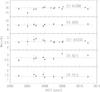 |
Fig. 1 Equivalent width of (from top to bottom) the CH λ4300, CN (0,0) R(0), CH+λ4232, CN R(1), and P(1) lines in ζ Per spectra between 2003 and 2011 (filled squares correspond to McD data and filled triangles to OHP data; error bars correspond to ± 1σ uncertainties). For each absorption feature, the horizontal line indicates the weighted average computed over all W values. |
As can be seen in Fig. 1, W values for CH and CN lines look essentially constant, as already noted in Boissé et al. (2009) for CH, earlier to 2009. To quantify this, we compute the weighted average, ⟨ W ⟩, and the rms dispersion around this value, σ, for each of these four series of measurements. We successively get :
-
⟨ W ⟩ = 15.96 ± 0.04 mÅ, σ = 0.34 mÅ for CH λ4300,
-
⟨ W ⟩ = 9.06 ± 0.06 mÅ, σ = 0.18 mÅ for CN R(0),
-
⟨ W ⟩ = 2.71 ± 0.06 mÅ, σ = 0.22 mÅ for CN R(1),
-
⟨ W ⟩ = 1.34 ± 0.06 mÅ, σ = 0.14 mÅ for CN P(1).
For CH+, Fig. 1 suggests a possible variation, with some hint of a maximum for W(CH+λ4232) between 2004 and 2007: inside this time interval, measurements tend to lie above the overall average while outside, they tend to fall below. The weighted average computed over all data values is ⟨ W ⟩ = 2.60 ± 0.04 mÅ, and the dispersion σ = 0.13 mÅ while we get ⟨ W ⟩ = 2.50 ± 0.07 mÅ and σ = 0.03 mÅ if values between 2004.0 and 2007.0 are excluded. We discuss the significance of this variation in more detail in Sect. 4.1.
Useful information is also contained in the line widths measured from McD spectra since the observed absorption lines are significantly broader than the line spread function. For instance, the b value measured for CH+ by Crane et al. (1995) is 2.3 km s-1 (this observation was performed between 1989 and 1992; here we implicitly assume that no important change in the line profile occurred later) while for R = 170 000, the corresponding “instrumental b value” is only 1.06 km s-1. At our resolution, the CH profile is consistent with a single Gaussian profile. To perform a meaningful comparison with the earlier data from Crane et al. (1995) who provide results for a two-component fit, we digitized their spectrum and performed a single component fit. We get an FWHM of 3.205 ± 0.025 km s-1, again significantly larger that the instrumental McD FWHM value (1.76 km s-1 for R = 170 000). Recall that due to Λ-doubling, the CH ground level is split into two sublevels (see e.g. Black & van Dishoeck 1988). The CH λ4300 profile is thus a blend of two transitions separated by 1.61 km s-1 (Bernath et al. 1991). When the splitting is taken into account (we assume equal populations for the two sublevels, in agreement with Jura & Meyer 1985), the b value implied by the observed FWHM of 3.20 km s-1 is b = 0.85 km s-1, consistent with the one (0.9 km s-1) given by Crane et al. (1995) for the main component considered in their fit. Regarding CN, Roth and Meyer (1995) found b = 1.125 ± 0.067 km s-1: the (0,0) band features are therefore only partially resolved in our spectra (these lines are in fact unresolved spin-rotation multiplets but the splittings are too small to significantly affect the CN profiles at our resolution). The accuracy of line width measurements for the P(1) CN feature is limited due to its weakness; we shall not consider these values in our study.
Examination of the measured line widths given in Table 1 shows that significant time variations are present. The CH and CN line width fluctuations display a strong mutual correlation. Since W values for these two species are constant, it is very likely that the CH and CN line width variations are due solely to changes in the spectral resolution, R, from one epoch to another. We do not have an accurate enough measure of R at each epoch that would allow us to check this statement and correct for the instrumental changes. But we can use the relatively strong CH λ4300 feature to track the variations in R and verify that the latter can account for time changes in the CN line widths. For Gaussian line profiles and LSF one can write:
 where FWHMobs(X,t) is the FWHM observed at time t for a line from species X, FWHMgas(X,t) is its intrinsic width and FWHMinst(X,t) the instrumental width, i.e. λ(X)/R(t) where λ(X) refers to the transition considered (here X ≡ CH+, CH, or CN). Note that, as explained above,
  (CH) does not directly reflect the velocity dispersion of the gas, due to the additional broadening induced by Λ-doubling.
Assuming that the CH λ4300 line width remained constant since the observation published by Crane et al. (1995) we have
 In the January 2003 McD spectrum, we measure FWHMobs = 3.70 ± 0.013 km s-1 from which we get for this epoch, R = 162 000. We then use this value to get the width for the deconvolved CH+ and CN profiles. We proceed similarly for each epoch and express our results for the deconvolved line widths in terms of the b velocity parameter.
In Fig. 2, we display the CH+, CN R(0), and R(1) deconvolved b values. The width of the strong CN R(0) line appears to be constant, in excellent agreement with our assumption that b(CH) did not vary. On the contrary, CH+b values tend to be higher around 2005, as with the case for W. The equivalent width of the CN R(1) line is quite similar to that of CH+λ4232 (see Fig. 1). It is thus noticeable that its behavior is fully consistent with that of the R(0) line, with no indication for a line width variation such as the one seen for CH+. It should be stressed that corrections for changes in R values remain limited and does not have a significant impact on the variation pattern observed for b(CH+). Computing the weighted average of b(CN), one gets ⟨ b ⟩ = 1.064 ± 0.014 km s-1 (this value is drawn from the more accurate R(0) line; for the R(1) feature, we get ⟨ b ⟩ = 1.022 ± 0.047 km s-1, in agreement with the R(0) estimate) a value in reasonably good agreement with the one obtained by Roth & Meyer (1995), b = 1.125 ± 0.067 km s-1.
 |
Fig. 2 Time variation of the b velocity parameter for the CH+λ4232 (red), CN R(0) (blue) and CN R(1) (green) lines towards ζ Per between 2003 and 2011 (the time for CN R(1) values have been shifted by + 0.1 yr to avoid confusion with CN R(0) points). The instrumental broadening has been corrected assuming that the CH line width remained constant and equal to the value inferred from the Crane et al. spectrum. The weighted average of b(CN) R(0) and R(1) values are shown (blue line for R(0); green line for R(1)). Both CN lines are consistent with a constant value while CH+ shows some increase around 2005. |
4. Discussion
4.1. Reality of the CH+ excess
To assess the significance of the excess noted for CH+ around 2005, we selected four epochs which correspond well to the interval when W values were higher (Oct. 04, Dec. 04, Oct. 05, and Dec. 05) and four others outside this interval (Jan. 03, Jan. 07, Jan. 08, Dec. 10; Jan. 04 was not considered because the accuracy is lower). We then compute the weighted average of W values in the excess interval (Win) and outside (Wout) and consider the relative difference  (3)for CH+, CH, and CN R(0) or R(1).
We get δW/W = 11.1 ± 4.4%,1.3 ± 0.6%, − 0.8 ± 1.4%, − 4.8 ± 4.5% for CH+, CH, CN R(0), and CN R(1) respectively. The excess for W(CH+) is significant at the 2.5σ level while no variation is seen for CN features. The CH value indicates a possible small excess; however, this result is to be taken with caution because at such low levels, it is difficult to rule out the presence of systematics.
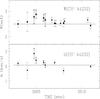 |
Fig. 3 Equivalent width of the CH+λ4232 line (upper panel) in ζ Per spectra between 2003 and 2011 (same symbols as in Fig. 1) together with the corresponding b value measured from high resolution McD data (lower panel). Thick error bars indicate measurements used to assess the significance of a maximum in W and b around (“in” values; see text). The b values have been corrected for instrumental broadening (see text). Note that both W and b display a maximum around 2005. In each panel, the horizontal line indicates the weighted average computed outside the time interval over which W was larger. |
Similar quantities (bin and bout) are computed for b values, corrected for instrumental broadening as explained above. For CH+, we get bin = 2.273 ± 0.084 km s-1, bout = 2.086 ± 0.057 km s-1 and ⟨ b ⟩ = 2.145 ± 0.047 km s-1, if the weighted average is computed over all data values. The relative variations are δb/b = 9.0 ± 4.9%, −1.1 ± 3.0%, −2.7 ± 9.6% for CH+, CN R(0), and CN R(1) respectively (recall that we have assumed δb(CH) = 0). The significance of the excess in b(CH+) is slightly smaller than for W. Figure 3 summarizes the CH+ results and illustrates the similarity between the trend observed for W and b.
Another way to assess the reality of the CH+ line variation is to compare the CH+ and CH line profiles in and out of the interval when W(CH+) reached its maximum. We accomplish this by computing the weighted average for the two sets of four spectra considered above (we use 1/σ2 weighting where σ is the rms value measured in the continuum adjacent to the absorption line). Since there remains some uncertainty (of about a few mÅ) in the wavelength scale of each spectrum, we aligned all line profiles to the same position before computing the average. The resulting CH+ and CH profiles are shown in Fig. 4 where we superimpose the “in” and “out” combined spectra (no correction was made for the slightly variable resolution from one epoch to another; the average resolution of “in” and “out” spectra being very similar, this effect cannot affect significantly the comparison). The two CH+ average profiles show a comparable central optical depth but the “in” line is noticeably broader, in agreement with the higher b value measured on the corresponding individual spectra. This increase in line width accounts for the higher W values observed in the 2004−2007 interval. Note that no such difference is discernable in the CH line profiles.
Given the good overall consistency between the behavior observed for W(CH+) and b(CH+) and the lack of any significant variation for CN lines of comparable strength, we conclude that the CH+ variation is most likely real. We have not discussed above possible changes in the line center. We measure changes of at most a few mÅ from one epoch to another for CH+, CH, and CN lines in McD spectra (1 mÅ corresponds to 0.07 km s-1 at 4000 Å); these apparent variations are comparable to the uncertainties in the wavelength scale. Only observations performed at very high resolution and with special care to get a very accurate absolute wavelength calibration could provide useful constraints on line shifts.
Before discussing the implications of our results on the CH+ production mechanism, we now mention some earlier CH+, CH, and CN measurements towards ζ Per that provide constraints on long term variations.
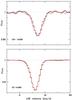 |
Fig. 4 CH+ (upper panel) and CH (lower panel) average normalized line profiles computed in the 2004−2007 interval during which W(CH+) reached a maximum (red) and outside this interval (black). The CH+ profile was slightly broader in the 2004−2007 interval, which accounts for higher W values. Note the excellent match of the two CH profiles. |
4.2. Variations on larger time scales
ζ Per being a bright star, several early but relatively accurate measurements of CH+, CH, and CN are available in the literature. One of the earliest CH+ values is that of Rogerson et al. (1959) who give for the CH+λ4232 line W = 5.2 ± 1.2 mÅ. Hobbs (1973) performed measurements down to 1 mÅ (sometimes 0.5 mÅ) and finds for ζ Per W = 3.2 mÅ and a FWHM of 3.9 km s-1 (observations made in 1971 and 1972 at R = 300 000). Chaffee (1974) gets W = 2: mÅ while Federman (1982) obtains 2.6 ± 0.9 mÅ (observations performed in 1979−1981). A decade later, Crane et al. (1995) finds W = 2.4 ± 0.2 mÅ and b = 2.2 km s-1 (spectra taken in the 1989−1992 interval). From our own study, outside the 2004−2007 interval, we get W = 2.50 ± 0.07 mÅ and b = 2.1 km s-1 (thus a FWHM of 3.5 km s-1). Clearly, the limited accuracy (uncertainties are not always provided by the authors) of the early measurements does not allow us to reveal variations as low as the one seen in our observations. Nevertheless, it is noticeable that the early values mentioned above do not suggest the existence of any large variation or systematic trend for an increase or decrease versus time.
Regarding the CH λ4300 line, Federman (1982) gives W = 15.9 ± 2.9 mÅ, while on the digitized version of Crane et al. spectrum, we measure W = 15.8 ± 0.3 mÅ. Both measurements are consistent with ours. Finally, a number of accurate CN measurements have been made in order to constrain the excitation of this species by interaction with the CMB radiation. Field & Hitchcock (1966) get W = 10.9 ± 1.1 mÅ and W = 3.5 ± 0.7 mÅ for the CN λ3874 R(0) and CN λ3873 R(1) lines. Meyer & Jura (1985) give W = 8.06 ± 0.07,2.51 ± 0.04, and 1.28 ± 0.04 for R(0), R(1), and P(1) respectively, while Kaiser & Wright (1990) obtain W = 8.93 ± 0.02,2.86 ± 0.02, and 1.35 ± 0.02 (weighted average values, as quoted by Roth & Meyer 1995). Finally, Roth & Meyer (1995) measure W = 9.06 ± 0.17,2.79 ± 0.17, and 1.36 ± 0.17 while we find W = 9.06 ± 0.06,2.71 ± 0.06, and 1.34 ± 0.06 mÅ. All these values are mutually consistent, except for the R(0) W measurement from Meyer & Jura (1985), which is probably due to a blend with a photospheric line. Thus, CH and CN features also appear to show no trend for an increase or decrease over several decades.
4.3. Observed variation and CH+ production models
Let us briefly summarize the main characteristics of the time evolution that emerges for CH+, CH, and CN from our study and from comparison with earlier data:
-
both the column density and the line width displayed no largevariation or systematic trend over the last 4−5 decades (corresponding to about 100 AU) for these 3 species,
-
over the 2003−2011 period, CH and CN features remained stable to a 3σ level better than 6% (this limit is drawn from the rms scatter of all values),
-
thanks to a tight sampling over the 2003−2011 period and to an improved accuracy in absorption line measurements, we detect a temporary 2.5σ increase of N(CH+) of 11% during the interval 2004−2007, accompanied by an increase in the line width of similar amplitude.
We now discuss the implications of the variation seen for CH+ in the context of models invoked to account for the abundance observed for this species. These models rely on the existence of localized regions inside which temperatures or ion-neutral relative drift velocities large enough to overcome the CH+ formation energy barrier are reached. Attributing the observed fluctuation in N and b to the passage through the line of sight of an individual structure, we can infer some characteristics of the latter:
-
i)
its size, l ≈ 2 to 7 AU (these values are derived from the range in drift velocities quoted in Sect. 2.2; an additional source of uncertainty is related to the unknown transverse velocity of the material which may contribute significantly to the relative drift),
-
ii)
the typical associated column density, δN(CH+) = 3 × 1011 cm-2.
Note that the stability of N(CH) is not inconsistent with the CH+ fluctuation. Some CH production is indeed directly associated with CH+, but the expected corresponding δN(CH) fluctuation should be comparable to δN(CH+), thus no larger than about N(CH)/100 (with N(CH) = 2.0 × 1013 cm-2 towards AE Aur). The limited accuracy of our measurements does not allow us to detect such weak variations. Adopting the rough assumption that all active regions are more or less identical and that the above values for l and δN(CH+) are representative of their properties, we can estimate that the number M of structures lying along the line of sight is M ≈ N(CH+)/δN(CH+) ≈ 10 and perform a comparison with model predictions.
In the following, we successively consider shocks and vortices. Another model involving transient microstructures has been proposed by Garrod et al. (1995) and Cecchi-Pestellini et al. (2009). These authors assume that perturbations generate transient dense knots of gas inside which complex chemistry can develop. However, the physical origin of these unbound tiny clumps is not specified in their model and therefore, the parameter values (the size in particular) remains largely arbitrary, preventing any detailed comparison with observations. We shall not consider this scenario further.
Let us first discuss shock models, as described by Flower & Pineau des Forêts (1998), Gredel et al. (2002), and more recently by Lesaffre et al. (2013). One difficulty in connecting their predictions to observations is that the 3D geometry of these regions is not well defined. One might imagine that they consist of a thin sheet (separating the pre-shocked and post-shocked gas) with a large transverse extent as observed for supernovae remnants or molecular outflows from young stellar objects. However, we are not dealing here with shocks induced by such large scale perturbations but rather by local supersonic fluctuations within the turbulent velocity field. Thus, a more realistic assumption in our context is that the lateral extent of a shocked region is comparable to its thickness (furthermore, numerical simulations of hydrodynamical shocks performed by Aota et al. 2013 indicate that the thermal instability leads to efficient fragmentation). We can then directly compare the size – a few AU – inferred from our observations to the thickness predicted by models. MHD shocks like those considered by Flower & Pineau des Forêts (1998) are characterized by a thickness of the order of 0.02 pc (or 4000 AU) and a column density of about 2 × 1012 cm-2 for a shock velocity us = 9 km s-1. Both values are much larger than those derived for the observed structure. One can also consider hydrodynamical shocks (i.e. shocks with small magnetic field B values or with B nearly parallel to the shock velocity). In the weakly magnetized case, Lesaffre et al. (2013) provide an estimate of 6 × 1013 cm or 4 AU for the thickness and a CH+ column density of 7 × 1010 cm-2 (we adopt their model with b = 0.1 and us = 12 km s-1). This latter value is to be considered as a lower limit since the column density is integrated along the normal to the shocked layer (if the latter has a non zero inclination i – the angle between the shock velocity and the line of sight – the column density will be larger by a factor 1/cosi). The model values are then reasonably close to our estimates for l and δN(CH+).
An alternative model involving turbulent vortices have been proposed by Joulain et al. (1998). Such structures are essentially 1D and the relevant size parameter is now the diameter of the vortices intersected by the line of sight. Godard et al. (2009) have described the physical and chemical properties of such active regions named “TDR” (for turbulent dissipation regions). In their Table 4, a model is considered for a density n = 100 cm-3, a reasonable value for the ζ Per line of sight, and an extinction by the ambient medium of Av = 0.4 mag. A CH+ column density of 6 × 1011 cm-2 is produced by 19 vortices with a characteristic scale of 20 AU, comparable to our constraint on l. Thus, in this model, a CH+ column density of about 3 × 1010 cm-2 is associated with each vortex. Such a column density is small compared to our δN(CH+) value but again, it is to be taken as a lower limit because if the filament is seen with some inclination i, the column density will be larger by of factor 1/cosi (with i = 0 for a filament lying in the plane of the sky). Furthermore, the properties of individual vortices strongly depend on model parameters, the rate of strain in particular, and larger column densities are certainly possible.
For both shock and vortex models, we can easily account for a broader CH+ line when W was at its maximum, just by adding along the sight line an active region whose bulk velocity is slightly offset with respect to the average velocity of the ≈10 others. Likewise, we note that in the vortex model, the passage of an additional filament through the line of sight should induce a specific signature in the absorption profile, depending on the rotation direction of the vortex and the viewing angle. The magnitude of the expected velocity perturbation is of the order of a few km s-1 (Godard et al. 2009; see their Fig. 2c). Given the weakness of the CH+ line towards ζ Per, observations with better S/N together with higher spectral resolution and accuracy in the wavelength calibration would be needed to reveal such effects (note that the change affects only ≈1/10 of this weak line). One may also wonder whether the good long term stability of W for the CH+λ4232 line is consistent with the small number (M ≈ 10) invoked for individual structures present along the sight line. If the latter are distributed at random in space, a Gaussian distribution is expected for the observed values of M. The probability of observing a deviation by more than 1σ, i.e. ΔM ≈ 3, corresponding to 1.7 mÅ ≤ W ≤ 3.2 mÅ, is about 0.3 (here, we used our value Wout = 2.50 mÅ). Clearly, given the limited accuracy of old measurements and their scarcity, M = 10 cannot be ruled out. We thus find that the characteristics of weakly magnetized shocks and vortices are roughly consistent with the observational constraints derived from our study.
We now conclude with some observational considerations. This work illustrates that the performances (temporal stability in particular) of presently available spectrographs is such that weak variations (at the percent level) of interstellar lines can now be studied in a systematic way in order to investigate in detail the small-scale structure of the ISM. In our discussion about shocks and vortex models, we are severely limited by the fact that we detected only one “variation event”. Sampling a larger area would clearly be important; this implies either observations over longer time intervals, or selecting targets with proper motions much larger than the one of ζ Per (this was the initial purpose of the HD 34078 project). Furthermore, when comparing observations to models, it would be quite helpful to have predictions for quantities that are directly accessible to this observational technique. For instance, extracting a cut through a vortex showing the expected time evolution of the CH+ column density and velocity distribution as the line of sight is drifting through the filament would be useful. This could allow us at the same time to better analyse the available data and to design observations which may be more appropriate to test the models. The velocity perturbations introduced by individual active regions are probably hardly accessible to optical spectroscopy; if modeling confirms this statement, radio observations of compact sources might be a better way to reach the required spectral resolution and velocity scale stability (species other than CH+ but tracing the same type of non-thermal chemistry and displaying radio transitions should then be used). These model predictions should cover the acceptable range for model parameters and consider various viewing angles.
Another directly observable property is the statistics of the N distribution. It would thus be important to determine from numerical modeling of a large enough sample of diffuse interstellar matter the expected statistics when a sight line drifts through an interstellar cloud. The computations needed to perform realistic predictions require a huge dynamical range (from the size of the whole region down to au scales) in order to correctly describe the physical and chemical properties of the tiny “active” structures that emerge within the chaotic velocity field. Such calculations are not yet feasible (for an example of recent MHD simulations of interstellar clouds, see Hennebelle 2013) but, in the near future, the fast increase in computer capabilities may bring results drawn from numerical simulations much closer to observational constraints like those presented in this paper.
Acknowledgments
We are grateful to the astronomers who have been involved in the acquisition of the OHP and McD observations as well as to the staff of these observatories for the excellent performance of the spectrographs. We also wish to thank Nicole Capitaine, Gary Mamon, Pasquier Noterdaeme and Yaron Sheffer for helpful discussions and comments. Several constructive remarks from the referee led to significant improvements in the final version of this paper.
References
- Aota, T., Inoue, T., & Aikawa, Y. 2013, ApJ, 775, 26 [NASA ADS] [CrossRef] [Google Scholar]
- Bernath, P. F., Brazier, C. R., Olsen, T., et al. 1991, J. Mol. Spectr., 147, 16 [NASA ADS] [CrossRef] [Google Scholar]
- Black, J. H., & van Dishoeck, E. F. 1988, ApJ, 331, 986 [NASA ADS] [CrossRef] [Google Scholar]
- Black, J. H., Hartquist, T. W., & Dalgarno, A. 1978, ApJ, 224, 448 [NASA ADS] [CrossRef] [Google Scholar]
- Bohlin, R. C. 1975, ApJ, 200, 402 [NASA ADS] [CrossRef] [Google Scholar]
- Boissé, P., Le Petit, F., Rollinde, E., et al. 2005, A&A, 429, 509 [NASA ADS] [CrossRef] [EDP Sciences] [Google Scholar]
- Boissé, P., Rollinde, E., Hily-Blant, P., et al. 2009, A&A, 501, 221 [NASA ADS] [CrossRef] [EDP Sciences] [Google Scholar]
- Cecchi-Pestellini, Williams, D. A., Viti, & Casu, S. 2009, ApJ, 706, 1429 [NASA ADS] [CrossRef] [Google Scholar]
- Chaffee, F. H., Jr 1974, ApJ, 189, 427 [NASA ADS] [CrossRef] [Google Scholar]
- Cordiner, M. A., Fossey, S. J., Smith, A. M., & Sarre, P. J. 2013, ApJ, 764, L10 [NASA ADS] [CrossRef] [Google Scholar]
- Crane, P., Lambert, D. L., & Sheffer, Y. 1995, ApJS, 99, 107 [NASA ADS] [CrossRef] [Google Scholar]
- Crawford, I. A. 2003, Astrophys. Space Sci., 285, 661 [Google Scholar]
- Falgarone, E., Pety, J., & Hily-Blant, P. 2009, A&A, 507, 355 [NASA ADS] [CrossRef] [EDP Sciences] [Google Scholar]
- Federman, S. R. 1982, ApJ, 257, 125 [NASA ADS] [CrossRef] [Google Scholar]
- Field, G. B., & Hitchcock, J. L. 1966, ApJ, 146, 1 [NASA ADS] [CrossRef] [Google Scholar]
- Flower, D. R., & Pineau des Forêts, G. 1998, MNRAS, 297, 1182 [NASA ADS] [CrossRef] [Google Scholar]
- Garrod, R. T., Williams, D. A., Hartquist, T. W., Rawlings, J. M. C., & Viti, S. 1995, MNRAS, 356, 654 [Google Scholar]
- Godard, B., Falgarone, E., & Pineau des Forêts, G. 2009, A&A, 495, 847 [NASA ADS] [CrossRef] [EDP Sciences] [Google Scholar]
- Gredel, R., Pineau des Forêts, G., & Federman, S. R. 2002, A&A, 389, 993 [NASA ADS] [CrossRef] [EDP Sciences] [Google Scholar]
- Hennebelle, P. 2013, A&A, 556, A153 [NASA ADS] [CrossRef] [EDP Sciences] [Google Scholar]
- Hobbs, L. M. 1973, ApJ, 181, 79 [NASA ADS] [CrossRef] [Google Scholar]
- Jenkins, E. B., & Tripp, T. M. 2011, ApJ, 734, 65 [NASA ADS] [CrossRef] [Google Scholar]
- Johnson, D. R. H., & Soderblom, D. R. 1987, AJ, 93, 864 [NASA ADS] [CrossRef] [Google Scholar]
- Joulain, K., Falgarone, E., Pineau des Forêts, G., & Flower, D. 1998, A&A, 340, 241 [NASA ADS] [Google Scholar]
- Jura, M., & Meyer, D. M. 1985, ApJ, 294, 238 [NASA ADS] [CrossRef] [Google Scholar]
- Kaiser, M. E., & Wright, E. L. 1990, ApJ, 356, L1 [NASA ADS] [CrossRef] [Google Scholar]
- Le Petit, F., Roueff, E., & Herbst, E. 2004, A&A, 417, 993 [NASA ADS] [CrossRef] [EDP Sciences] [Google Scholar]
- Lesaffre, P., Pineau des Forêts, G., Godard, B., et al. 2013, A&A, 550, A106 [NASA ADS] [CrossRef] [EDP Sciences] [Google Scholar]
- Moore, E. M., & Marscher, A. P. 1995, ApJ, 452, 671 [NASA ADS] [CrossRef] [Google Scholar]
- Meyer, D. M., & Jura, M. 1985, ApJ, 297, 119 [NASA ADS] [CrossRef] [Google Scholar]
- Pan, K., Federman, S. R., & Welty, D. E. 2001, ApJ, 558, L105 [NASA ADS] [CrossRef] [Google Scholar]
- Rogerson, J. B., Spitzer, L., & Bahng, J. D. 1959, ApJ 130, 991 [Google Scholar]
- Roth, K. C., & Meyer, D. M. 1995, ApJ, 441, 129 [NASA ADS] [CrossRef] [Google Scholar]
- Roy, N., Minter, A. H., Goss, W. M., Brogan, C. L., & Lazio, T. J. W. 2012, ApJ, 749, 144 [NASA ADS] [CrossRef] [Google Scholar]
- Savage, B. D., Bohlin, R. C., Drake, J. F., & Budich, W. 1977, ApJ, 216, 291 [NASA ADS] [CrossRef] [Google Scholar]
- Schönrich, R., Binney, J., & Dehnen, W. 2010, MNRAS, 403, 1829 [NASA ADS] [CrossRef] [Google Scholar]
- Shaw, G., Ferland, G. J., Abel, N. P., et al. 2008, ApJ, 675, 405 [NASA ADS] [CrossRef] [Google Scholar]
- Sheffer, Y., Rogers, M., Federman, S. R., Lambert, D. L., & Gredel, R. 2007, ApJ, 667, 1002 [NASA ADS] [CrossRef] [Google Scholar]
- Sheffer, Y., Rogers, M., Federman, S. R., et al. 2008, ApJ, 687, 1075 [NASA ADS] [CrossRef] [Google Scholar]
- Smith, K. T., Fossey, S. J., Cordiner, M. A., et al. 2013, MNRAS, 429, 939 [NASA ADS] [CrossRef] [Google Scholar]
- van Leeuwen, T. 2007, A&A, 474, 653 [NASA ADS] [CrossRef] [EDP Sciences] [Google Scholar]
- Welty, D. E., Thuson, Simon, & Hobbs, L. M. 2008, MNRAS, 388, 323 [NASA ADS] [CrossRef] [Google Scholar]
All Tables
List of McD (M) and OHP (O) observations with measured CH+ λ4232, CH λ4300 and CN (0,0) R(1), R(0), and P(1) line equivalent width (W) and full width at half maximum (FWHM; for CN P(1) McD observations, no FWHM is given because of low accuracy).
All Figures
|
Fig. 1 Equivalent width of (from top to bottom) the CH λ4300, CN (0,0) R(0), CH+λ4232, CN R(1), and P(1) lines in ζ Per spectra between 2003 and 2011 (filled squares correspond to McD data and filled triangles to OHP data; error bars correspond to ± 1σ uncertainties). For each absorption feature, the horizontal line indicates the weighted average computed over all W values. |
| In the text | |
|
Fig. 2 Time variation of the b velocity parameter for the CH+λ4232 (red), CN R(0) (blue) and CN R(1) (green) lines towards ζ Per between 2003 and 2011 (the time for CN R(1) values have been shifted by + 0.1 yr to avoid confusion with CN R(0) points). The instrumental broadening has been corrected assuming that the CH line width remained constant and equal to the value inferred from the Crane et al. spectrum. The weighted average of b(CN) R(0) and R(1) values are shown (blue line for R(0); green line for R(1)). Both CN lines are consistent with a constant value while CH+ shows some increase around 2005. |
| In the text | |
|
Fig. 3 Equivalent width of the CH+λ4232 line (upper panel) in ζ Per spectra between 2003 and 2011 (same symbols as in Fig. 1) together with the corresponding b value measured from high resolution McD data (lower panel). Thick error bars indicate measurements used to assess the significance of a maximum in W and b around (“in” values; see text). The b values have been corrected for instrumental broadening (see text). Note that both W and b display a maximum around 2005. In each panel, the horizontal line indicates the weighted average computed outside the time interval over which W was larger. |
| In the text | |
|
Fig. 4 CH+ (upper panel) and CH (lower panel) average normalized line profiles computed in the 2004−2007 interval during which W(CH+) reached a maximum (red) and outside this interval (black). The CH+ profile was slightly broader in the 2004−2007 interval, which accounts for higher W values. Note the excellent match of the two CH profiles. |
| In the text | |
Current usage metrics show cumulative count of Article Views (full-text article views including HTML views, PDF and ePub downloads, according to the available data) and Abstracts Views on Vision4Press platform.
Data correspond to usage on the plateform after 2015. The current usage metrics is available 48-96 hours after online publication and is updated daily on week days.
Initial download of the metrics may take a while.