| Issue |
A&A
Volume 559, November 2013
|
|
|---|---|---|
| Article Number | A48 | |
| Number of page(s) | 20 | |
| Section | Planets and planetary systems | |
| DOI | https://doi.org/10.1051/0004-6361/201322284 | |
| Published online | 11 November 2013 | |
A survey of volatile species in Oort cloud comets C/2001 Q4 (NEAT) and C/2002 T7 (LINEAR) at millimeter wavelengths ⋆,⋆⋆,⋆⋆⋆
1
Max Planck Institute for solar system Research,
Max-Planck-Str. 2, 37191
Katlenburg-Lindau,
Germany
e-mail: This email address is being protected from spambots. You need JavaScript enabled to view it.
;rezac;This email address is being protected from spambots. You need JavaScript enabled to view it.
2
Department of Astrophysical Sciences, Princeton
University, Princeton, NJ
08544,
USA
e-mail: This email address is being protected from spambots. You need JavaScript enabled to view it.
3
Rosetta Science Operations Centre, European Space Astronomy
Centre, European Space Agency, PO
Box 78, 28691 Villanueva de la Cañada, Madrid, Spain
e-mail: This email address is being protected from spambots. You need JavaScript enabled to view it.
4
LESIA, Observatoire de Paris, CNRS, UPMC, Université
Paris-Diderot, 5 place Jules
Janssen, 92195
Meudon,
France
e-mail:
This email address is being protected from spambots. You need JavaScript enabled to view it.
; This email address is being protected from spambots. You need JavaScript enabled to view it.
; This email address is being protected from spambots. You need JavaScript enabled to view it.
5
solar system Exploration Division, NASA Goddard Space Flight Center, Greenbelt, MD
20771,
USA
e-mail: This email address is being protected from spambots. You need JavaScript enabled to view it.
6
Department of Physics, Catholic University of
America, Washington,
DC
20064,
USA
Received:
15
July
2013
Accepted:
1
August
2013
Abstract
Context. The chemical composition of comets can be inferred using spectroscopic observations in submillimeter and radio wavelengths.
Aims. We aim to compare the production rates ratio of several volatiles in two comets, C/2001 Q4 (NEAT) and C/2002 T7 (LINEAR), which are generally regarded as dynamically new and likely to originate in the Oort cloud. This type of comets is considered to be composed of primitive material that has not undergone considerable thermal processing.
Methods. The line emission in the coma was measured in the comets, C/2001 Q4 (NEAT) and C/2002 T7 (LINEAR), that were observed on five consecutive nights, 7–11 May 2004, at heliocentric distances of 1.0 and 0.7 AU, respectively, by means of high-resolution spectroscopy using the 10-m Submillimeter Telescope at the Arizona Radio Observatory. Both objects became very bright and reached naked-eye visibility during their perihelion passage in the spring of 2004.
Results. We present a search for six parent- and product-volatile species (HCN, H2CO, CO, CS, CH3OH, and HNC) in both comets. Multiline observations of the CH3OH J = 5–4 series allow us to estimate the rotational temperature using the rotation diagram technique. We derive rotational temperatures of 54(9) K for C/2001 Q4 (NEAT) and 119(34) K for C/2002 T7 (LINEAR). The gas production rates are computed using the level distribution obtained with a spherically symmetric molecular excitation code that includes collisions between neutrals and electrons. The effects of radiative pumping of the fundamental vibrational levels by infrared photons from the Sun are considered for the case of HCN. We find an HCN production rate of 2.96(5) × 1026 molec.s-1 for comet C/2001 Q4 (NEAT), corresponding to a mixing ratio with respect to H2O of 1.12(2) × 10-3. The mean HCN production rate during the observing period is 4.54(10) × 1026 molec.s-1 for comet C/2002 T7 (LINEAR), which gives a mixing ratio of 1.51(3) × 10-3. Relative abundances of CO, CH3OH, H2CO, CS, and HNC with respect to HCN are 3.05(83) × 101, 1.50(25) × 101, 1.16(27), 7.02(30) × 10-1, and 5.75(73) × 10-2 in comet C/2001 Q4 (NEAT) and <4.12 × 101, 4.07(44) × 101, 4.72(73), 1.32(6), and 1.09(8) × 10-1 in comet C/2002 T7 (LINEAR).
Conclusions. With systematically lower mixing ratios in comet C/2001 Q4 (NEAT), production rate ratios of the observed species with respect to H2O lie within the typical ranges of dynamically new comets in both objects. We find a relatively low abundance of CO in C/2001 Q4 (NEAT) compared to the observed range in other comets based on millimeter/submillimeter observations, and a significant upper limit on the CO production in C/2002 T7 (LINEAR) is derived. Depletion of CO suggests partial evaporation from the surface layers during previous visits to the outer solar system and agrees with previous measurements of dynamically new comets. Rotational temperatures derived from CH3OH rotational diagrams in both C/2001 Q4 (NEAT) and C/2002 T7 (LINEAR) are roughly consistent with observations of other comets at similar distances from the Sun.
Key words: comets: individual: C/2002 T7 (LINEAR) / comets: individual: C/2001 Q4 (NEAT) / submillimeter: planetary systems / techniques: spectroscopic / molecular processes
Based on observations acquired with the 10-m Submillimeter Telescope at the Arizona Radio Observatory, Steward Observatory, Mount Graham, Arizona, USA.
Tables 3 and 4 are available in electronic form at http://www.aanda.org
Full Tables 7, 8, and reduced spectra as FITS files are only available at the CDS via anonymous ftp to cdsarc.u-strasbg.fr (130.79.128.5) or via http://cdsarc.u-strasbg.fr/viz-bin/qcat?J/A+A/559/A48
© ESO, 2013
1. Introduction
Having spent most of their lifetime in the cold outer regions of the solar system, comets contain pristine material that have not evolved very much since their formation. Therefore, the composition of cometary nuclei reflects that of the early solar nebula; characterizing their chemical conditions can help to constrain planetary formation models. Spectroscopic observations of cometary atmospheres at various wavelengths are an efficient tool for investigating the physical and chemical diversity of comets, and substantial efforts have been made in the last two decades to develop a chemical classification of comets that displays a great compositional diversity (A’Hearn et al. 1995; Biver et al. 2002; Bockelée-Morvan et al. 2004; Bockelée-Morvan 2011). These observations reveal critical information about the composition of the primordial material in the solar nebula and the early formation stages of the solar system. In addition, studying the role of the volatile ice composition in the sublimation of material from the surface is important in the understanding of cometary activity.
According to the standard dynamical model (see Rickman 2010, for a comprehensive review of cometary dynamics), Oort cloud comets are believed to have formed in the giant planet region between Jupiter and Neptune before being ejected to the outer regions of the Solar Nebula. However, it has been speculated that a fraction of the objects in the Oort cloud have been captured from other stars in the vicinity of the Sun during its formation (Levison et al. 2010). Objects in the Oort cloud are occasionally perturbed by passing stars or galactic tides and injected into the inner solar system. Although the present cometary impact rates are low, several collisions of km-sized bodies have occurred in Jupiter in recent years since the Shoemaker-Levy 9 impact in 1994, which produced large atmospheric disturbances (see e.g. Sánchez-Lavega et al. 2010; Cavalié et al. 2013).
Conversely, Jupiter-family comets (JFC) form by accretion in a different region, the Edgeworth-Kuiper belt, beyond Neptune’s orbit up to about 100 AU from the Sun. Although Oort cloud comets were probably assembled on average closer to the Sun, observations of the abundance of cometary volatiles suggest that there could have been mixing of material and an overlap of the regions, where both kind of objects formed (Bockelée-Morvan et al. 2004; Bockelée-Morvan 2011; A’Hearn et al. 2012). Dynamical simulations also indicate that formation of a fraction of the JFC and Oort cloud comet populations can occur in the transneptunian scattered disk region, where they could be gravitationally scattered by the giant planets (Rickman 2010).
In addition to several radicals and ions formed by photodissociation in the coma, more than 20 different volatile species have been detected via ground-based spectroscopic surveys at infrared to millimeter wavelengths and measured in situ in comets belonging to different dynamical families. Many of these molecules are parent species that originate directly in the nucleus ices and play an important role in organic chemistry (e.g. H2O, HCN, and CH3OH). The composition of some cometary ices show strong evidence of processing in the solar nebula and can provide clues about their place of formation and subsequent evolution. Submillimeter observations using heterodyne receivers can be used to resolve the line shape and enable the determination of accurate production rates with the aid of a molecular excitation code (e.g., Biver et al. 2002). Moreover, the coma structure and outgassing velocity can be derived by fitting the observed line shapes, and mixing ratios of volatile species can be compared to observed chemical abundances in protoplanetary disks to improve our understanding of the formation and evolution of the solar system. However, there is no evident systematic correlation between the observed relative abundances and the dynamical class of the comets (see e.g. A’Hearn et al. 2012); therefore studying a larger sample of comets is needed.
We have derived the production rates for the observed molecular lines in the bright comets C/2001 Q4 (NEAT) and C/2002 T7 (LINEAR) during their 2004 apparitions and compared them to the mixing ratios measured in other comets. In Sect. 2, the observations of several volatile species, namely HCN, H2CO, CO, CS, CH3OH, and HNC, that were first reported by Küppers et al. (2004) and Villanueva et al. (2005), and the reduction method are summarized. Section 3 presents the data analysis of the observations using the molecular excitation calculated with a code based on ratran (Hogerheijde & van der Tak 2000; Bensch & Bergin 2004) and discusses the derived production rates for the detected molecules and the short-term time variability of the HCN production rates. Finally, we summarize the obtained results and discuss the main conclusions in Sect. 4.
2. Observations
A spectral line survey of primary and daughter volatile species in comets C/2002 T7 (LINEAR) and C/2001 Q4 (NEAT) was made in 7–11 May 2004 using the Submillimeter Telescope (SMT; Baars & Martin 1996; Baars et al. 1999, formerly known as the Heinrich Hertz Submillimeter Telescope) located at the Mount Graham International Observatory (MGIO), a division of Steward Observatory on Mount Graham, Arizona (latitude 32°42′05 8 N, longitude 109°53′285 W and elevation 3186 m). The SMT telescope has a parabolic 10-m primary dish and a hyperbolic nutating secondary reflector. Several sensitive heterodyne receivers and backends are available that allow deep line searches with a broad frequency coverage. The observations presented here were performed in remote observing mode using the 1.3 mm double sideband superconductor-insulator-superconductor (SIS) receiver system using various spectrometers. This receiver allows us to observe horizontal and vertical polarizations simultaneously and to improve the signal-to-noise ratio (S/N) by averaging data from both polarization channels.
The main goal of our observing program was to obtain the relative abundances of the dynamically new comets C/2001 Q4 (NEAT) and C/2002 T7 (LINEAR) and to confront them with the composition of dynamically old ones, such as comet C/2004 Q2 (Machholz) that was also observed at the SMT (de Val-Borro et al. 2012a). An additional purpose of these observations was to test the performance and stability of the newly installed high-resolution chirp transform spectrometer (CTSB) built at the Max Planck Institute for solar system Research (Hartogh & Hartmann 1990; Hartogh 1997a,b; Villanueva & Hartogh 2004; Villanueva et al. 2006) and to compare these observations to the results from the acousto-optical spectrometers. High spectral resolution is crucial for resolving the shape of rotational lines in comets and for studying the gas velocity and asymmetries related to non-isotropic outgassing and self-absorption effects. Therefore, the CTSB spectrometer has been used in parallel with other spectrometers in several cometary observation programs at the SMT, since its installation in early 2004 (see e.g. Küppers et al. 2004; Villanueva et al. 2005; Drahus et al. 2010; Paganini et al. 2010; Jockers et al. 2011; de Val-Borro et al. 2011, 2012a).
We observed the comet simultaneously with the Forbes filterbanks (F1.M and F250) with bandwidths of 2 GHz and 64 MHz, the CTSB with a bandwidth of 215 MHz, and the acousto-optical spectrometers (AOSA, AOSB, and AOSC) with total bandwidths of 1 GHz, 970 MHz, and 250 MHz, respectively. The spectral resolution provided was 1 MHz and 250 kHZ for the F1.M and F250 filterbanks; 40 kHz for the CTSB; and 934 kHz, 913 kHz and 250 kHz for the AOSA, AOSB, and AOSC, respectively. A typical system temperature of 1200 K was attained with ~40% fluctuations during the observing period. We focus on the observations acquired with the AOSA, AOSB, and CTSB backends.
We performed pointing and focus calibration on Saturn, Mars, and Uranus, because they were close to the comets during the course of our observations. Flux density reference observations of bright standard sources, like the evolved star IRC +10216, the protobinary system W3(OH), and the protoplanetary nebula CRL 2688, were obtained interleaved with the comet observations for calibration purposes.
We used the latest osculating orbital elements provided by JPL’s HORIZONS online solar system data service1 during the observations to track the position and relative motion of the comet with respect to the observer (Giorgini et al. 1996). Typical telescope pointing errors were ~2″ during our observing run and were included in the derivation of the production rates.
2.1. Comet C/2001 Q4 (NEAT)
Comet C/2001 Q4 (NEAT), hereafter referred to as C/2001 Q4, is generally considered a dynamically new comet, which is likely to originate in the Oort cloud and is visiting the inner solar system for the first time. It was discovered on 24 August 2001 as a 20th magnitude object at a heliocentric distance of 10.1 AU by the Near-Earth Asteroid Tracking (NEAT) program using the 1.2-m Samuel Oschin telescope at Palomar observatory (Pravdo et al. 2001). Comet C/2001 Q4 reached perihelion on 16 May 2004 at a distance of 0.962 AU from the Sun and had its closest approach to Earth on 7 May 2004 at a distance of 0.32 AU. Spectral observations of C/2001 Q4 were carried out shortly before perihelion from 7 to 11 May 2004 using the SMT. We searched for several rotational lines of molecular species (namely HCN, H2CO, CO, CS, CH3OH, and HNC) using the position-switching observing mode with a 0 5 offset in azimuth. Water was first detected on 6 March 2004 with a production rate of QH2O = 1.79(55) × 1029 molec.s-1 as measured by the Odin satellite (Lecacheux et al. 2004; Biver et al. 2009). From the periodic variations in the outgassing rate of the 557 GHz H2O line, Biver et al. (2009) derived a rotation period of 0.816(4) days. The comet showed an asymmetry in the overall outgassing activity with a peak about two weeks before perihelion (Combi et al. 2009; Biver et al. 2009).
2.2. Comet C/2002 T7 (LINEAR)
Comet C/2002 T7 (LINEAR), hereafter C/2002 T7, was discovered on 14 October 2002 at 6.9 AU by the Lincoln Near-Earth Asteroid Research (LINEAR) project with a visual magnitude of 17.5 (Birtwhistle & Spahr 2002). This comet is also regarded as a dynamically new Oort cloud object with a slightly hyperbolic orbit at perihelion. It passed perihelion on 23 April 2004 at a heliocentric distance of 0.61 AU and reached perigee on 19 May 2004 at 0.27 AU from the Earth. We observed C/2002 T7 on 8–11 May 2004 at the SMT when the comet was at heliocentric distance of ~0.72 AU and 0.45 from the Earth. Due to its favorable geometry for observations from Earth, a large number of volatile species have been found in this comet from infrared, submillimeter and radio observational campaigns (Friedel et al. 2005; DiSanti et al. 2006; Milam et al. 2006; Remijan et al. 2008; Hogerheijde et al. 2009).
Log of the observed rotational transitions in comets C/2001 Q4 (NEAT) and C/2002 T7 (LINEAR) in our SMT observing campaign from 7 to 11 May 2004.
2.3. Data reduction
The observed antenna temperature scale,  , was calibrated using the chopper-wheel method with the on-site data processing software (see Ulich & Haas 1976), and the combined dataset was stored using the Continuum and Line Analysis Single-dish Software (CLASS) file type. Moreover, we have corrected the temperature scale for the average beam efficiency of the telescope, which is estimated to be ηB = 0.74(2) from observations of Mars and Saturn in the fall 2007–spring 20082. This gives
  , where
  is the antenna temperature corrected for atmospheric attenuation, radiative loss, rearward scattering, and spillover losses. The reduction of the SMT spectra was performed using the open-source pyspeckit spectroscopic toolkit written in Python, which depends on the NumPy library (Oliphant 2006) for manipulating multidimensional arrays efficiently (Ginsburg & Mirocha 2011). The pyspeckit package supports many file types including some versions of the non-standard CLASS file format3.
Table 1 summarizes the frequencies of the molecular species transitions, observing dates, comet distances, and beam sizes in comets C/2001 Q4 (NEAT) and C/2002 T7 (LINEAR) during our observing run at the SMT.
The data analysis was carried out as described by de Val-Borro et al. (2012a). A standing wave appears as a baseline ripple in the observed spectra. Using the Lomb-Scargle periodogram technique, the baseline was removed by fitting a linear combination of sine waves to the emission-free background and subtracted from the original spectrum. This method has the advantage that it can be applied to unevenly spaced series, as in the case when the narrow emission features are masked in the spectra before fitting the baseline. Using alternative methods to fit standing wave, such as the Hilbert-Huang transform (HHT), give similar results (Rezac et al., in prep.). After removal of the baseline ripple, the individual scans were averaged to increase the S/N. Line intensities were calculated from the weighted averages of the spectra, where the statistical weights of each individual spectrum are proportional to the exposure time and inversely proportional to the system temperature squared.
The statistical uncertainty in the integrated line intensity was calculated using the root mean square (rms) noise in the background after subtracting the fitted baseline. Detected emission lines may have a different gain response, depending upon which sideband the lines were observed in. Thus, the sideband gain ratio between the upper and lower sidebands (GUSB/GLSB) deviates from unity and introduces an additional uncertainty of ~10% in the absolute brightness temperature calibration (de Val-Borro et al. 2012a).
3. Results
3.1. Excitation model
To compute the production rates, we adopted a radiative transfer code based on ratran (Hogerheijde & van der Tak 2000; Hogerheijde et al. 2009) that includes collisions between neutrals and electrons and radiation trapping effects (see de Val-Borro et al. 2010, and references therein). The radiative pumping of the fundamental vibrational levels, which are induced by solar infrared radiation and subsequently decay to rotational levels in the ground vibrational state, is considered only for the case of HCN. We used the one-dimensional spherically symmetric version of the code with a constant outflow velocity by following the description outlined in Bensch & Bergin (2004), which has been used to model water excitation to interpret Herschel cometary observations (see e.g. Bockelée-Morvan et al. 2010, 2012; de Val-Borro et al. 2012b; O’Rourke et al. 2013).
Although the outgassing rate may be variable on short timescales due to the rotation of the nucleus as discussed in Sect. 3.5, an isotropic steady-state radial gas density profile for parent molecules was assumed using the standard Haser spherically symmetric distribution (Haser 1957):  (1)where Q is the total production rate in molecules s-1, vexp is the expansion velocity, and r is the nucleocentric distance. Volatiles that sublimate off the surface of the comet can be photodissociated when they are exposed to solar UV radiation; the photodissociation rate β considers the dissociation and ionization of molecules by the radiation from the Sun and determines the spatial distribution of the species.
Photodissociation rates from the quiet-Sun reference spectrum at 1 AU for the observed molecules and corresponding scale-lengths in C/2001 Q4 and C/2002 T7 at rh = 0.97 and 0.72 AU, respectively.
We obtained the photodissociative lifetimes for CH3OH, HCN, H2CO, and CO at 1 AU from Crovisier (1994) assuming the quiet-Sun reference spectrum, and the HNC and CS radical lifetimes were taken from Biver et al. (2011). Photodissociation rates and scale-lengths for the observed species are summarized in Table 2. The photodissociation rates were scaled by the heliocentric distance of the comets as  at the time of the observations. Nevertheless, some daughter molecules, such as CS, HNC, and H2CO, are not correctly described by the Haser parent molecule profile. The density profile of daughter species originating from the photodissociation of an extended parent source in the coma is taken from Combi et al. (2004). We use a distributed source in the coma with parent species photodissociation rates at 1 AU of β0,p = 1 × 10⁻⁴ s-1 and 1.7 × 10⁻³ s-1 for H2CO and CS, respectively (see de Val-Borro et al. 2012a, and references therein). There are no constraints on the scale-length and distribution of HNC in the comae of comets C/2001 Q4 and C/2002 T7. Thus, we assumed a parent molecule profile for HNC to compute the production rates.
The excitation conditions of molecules in cometary atmospheres have been studied initially by Crovisier & Encrenaz (1983) and Crovisier (1984). Neutrals are excited by collisions with mainly water molecules and electrons, which are the dominant effects in the inner coma. For HCN, the radiative pumping of the fundamental vibrational levels by the solar infrared flux has been included. Infrared pumping of vibrational bands by solar radiation becomes the dominant excitation mechanism in the outer coma, where the gas and electron densities are low and their collision rates become negligible (Bockelée-Morvan 1987). For a beam size of about 30′′ at the observed frequencies, we are probing a region where excitation is mainly dominated by collisions and the level populations can be described approximately by a Boltzmann distribution at the gas kinetic temperature.
Water is the main volatile component of cometary nuclei and is typically used to determine relative abundances. Although water is not directly accessible from the ground at submillimeter wavelengths, it has been observed from space using the Odin and Herschel satellites (see Lecacheux et al. 2003; Hartogh et al. 2010, 2011; Biver et al. 2012). The water production rate of comet C/2001 Q4 derived from Odin observations between 2 April and 16 May 2004 has a long-term variation that depends on the heliocentric distance and seasonal effects. A Gaussian fit of the daily average of the outgassing rates is given by (Biver et al. 2009): 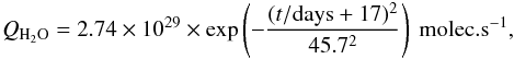 (2)where t is the time in days relative to C/2001 Q4’s perihelion passage, UT 15.97 May 2004. The values obtained from this formula at the time of the SMT observations have been used in our excitation model and to calculate the mixing ratios with respect to H2O. We used a water production rate of QH2O = 3 × 1029 molec.s-1 for comet C/2002 T7 at the time of our observations, which are derived from the observation of the fundamental H2O transition at 557 GHz with the Odin satellite at different heliocentric distances (Biver et al. 2007b).
The outgassing velocity in the coma is assumed to be constant in our model with values of 0.73 km s-1 for comet C/2001 Q4 and 0.90 km s-1 for comet C/2002 T7. These values were obtained from the half-width-at-half maximum (HWHM) of a single Gaussian function fitted to the HCN line observed by the CTSB, whose line profiles are relatively symmetric and have the highest S/N of the detected transitions. The HWHM was further reduced by 10% to consider the increase in line width due to thermal Doppler broadening (e.g. Biver et al. 1997). The HCN line width decreases by ~5% from UT 8.68 to 11.60 May in comet C/2002 T7, and the value for the outflow velocity above has been derived from the weighted average of the HCN spectra on three different dates. We also provide for reference the values of the expansion velocities of the other lines in Tables 3 and 4 for both objects.
The distribution of rotational levels in the collisional region is given by the gas neutral temperature that is assumed to be equal to the rotational temperature. We estimated the rotational temperatures in both comets from the relative intensities of the measured CH3OH transitions as described in Sect. 3.2.
We chose an electron density scaling factor of xne = 0.2 with respect to the reference profile deduced from in situ measurements of comet 1P/Halley as defined by Biver (1997) and Biver et al. (1999, 2007b). The electron density distribution in comet C/2001 Q4 is constrained by the brightness distribution of the 557 GHz line of H2O that was mapped by the Odin satellite with high spatial resolution on 16 May 2004 (Biver et al. 2007b). This scaling factor minimizes the radial variation between production rates derived from the intensity at various offset points. For C/2002 T7, we used the same value for the electron density scaling factor, since its density distribution has not been estimated by mapping observations.
 |
Fig. 1 Upper panel: CH3OH averaged spectrum toward comet C/2001 Q4 (NEAT) acquired on UT 11.03 May 2004 with a 312 min total integration time using the AOSA (thick blue line) and AOSB (thin red line). Lower panel: frequency range covered by the CTSB (black line) with the AOSA (thick blue line) and AOSB (thin red line) spectra. The lower sideband frequency is shown in the horizontal axes and the calibrated main beam brightness temperature in the vertical axes. The CTSB spectrum was resampled to a 190 kHz resolution per channel with a rectangular window function to increase the S/N of the detected lines. Note that a spurious emission feature is present around 241.825 GHz in the AOSA spectrum. The rms noise level in the main brightness temperature is calculated from the background level and is shown by the blue, red, and gray bars on the right of the lower panel for AOSA, AOSB, and CTSB, respectively. Note that the rms in the CTSB spectrum was calculated for the native frequency resolution of 40 kHz. |
3.2. Rotational temperatures
Methanol rotational transitions appear in several multiplets at millimeter wavelengths that are well suited to estimate the rotational temperature and excitation conditions in the coma in the optically thin limit. The rotational levels of CH3OH listed in Table 1 are described with three quantum numbers (JK Ts) following the notation by Mekhtiev et al. (1999), where J is the total angular momentum, K its projection along the symmetry axis, and Ts is the torsional symmetry state (A, A, E1 or E2). The difference between the E1 and E2 states is indicated by the sign of the quantum number K with a positive sign corresponding to E1 levels and a negative sign to E2 levels. All the observed transitions in comets C/2001 Q4 and C/2002 T7 are in the first torsional state (quantum number νt = 0).
The rotational temperature was derived using the rotational diagram (also known as Boltzmann diagram) technique, which is frequently used in studies of the interstellar medium, from the relative intensities of the individual CH3OH lines between levels with quantum numbers J = 5–4. We assume that the population distribution of the levels sampled by the emission lines is in local thermodynamical equilibrium (LTE), or described by a Boltzmann distribution characterized by a single temperature. Then the column density of the upper transition level within the beam, ⟨ Nu ⟩, can be expressed as  (3)where gu is the degeneracy of the upper level, Z denotes the rotational partition function, which is a function of temperature, Trot is the rotational temperature, Eu is the energy of the upper state, kB represents the Boltzmann constant, and ⟨ N ⟩ is the total column density averaged over the beam (see Bockelée-Morvan et al. 1994).
For optically thin conditions that normally apply to cometary lines of most volatile species, the line intensity,  , is proportional to the averaged column density in the upper level of the observed transition within the beam:
 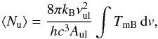 (4)where νul is the transition frequency, h denotes the Planck constant, c is the speed of light and Aul the Einstein coefficient for spontaneous emission. This relation assumes that the beam sizes of the observed transitions are approximately the same. Although the observed transitions in C/2001 Q4 and C/2002 T7 are at nearby frequencies, the excitation energy of the upper level varies between 35 and 85 K, which allows us to retrieve the rotational temperature using the rotational diagram method. As noted by Bockelée-Morvan et al. (1994), (see also Biver et al. 2002), it is best to use CH3OH lines in which ΔJ = 0 and ΔK ≠ 0; in this case we have ΔJ ≠ 0 and ΔK = 0, which makes these lines sensitive to deviations from LTE.
3.2.1. Comet C/2001 Q4 (NEAT)
Figure 1 shows the CH3OH rotational transitions (J = 5–4) observed in the lower sideband in comet C/2001 Q4. Ten transitions are detected by the AOSA and AOSB backends, including three blended lines around 241.833, 241.843, and 241.904 GHz that are designated by the dashed lines. Seven of those transitions are also detected in the frequency range covered by the CTSB (see lower panel in Fig. 1). To increase the S/N of the CTSB spectra, we resampled over four adjacent channels with a rectangular window function corresponding to an effective spectral resolution of 190 kHz. Additionally, the CTSB spectrum shows tentative detections of the 54–44 E, 5-3–4-3 E and 52–42 A+ transitions at 241.829, 241.852 and 241.887 GHz, respectively, that are also indicated by vertical dashed lines. The 54–44 E transition is marginally detected in both AOSA and AOSB backends as well, but since the line is very close to a blended pair, the baseline subtraction technique cannot be performed reliably.
We show the best fit of the rotational diagram for all lines observed in comet C/2001 Q4 with the AOSA, AOSB, and CTSB spectrometers in Fig. 2. The rotation diagram fits all detected CH3OH lines using a weighted linear least-squares method, where the weights are equal to the reciprocal of the variance of each measurement. A rotational temperature of 54(9) K is obtained from the best linear fit to the transitions detected above the 3-σ detection limit with all the spectrometers. In comparison, a rotational temperature of Trot = 70 × (rh/AU)-1 K is derived from the relative line intensities of CH3OH lines observed at the Institut de Radioastronomie Millimétrique (IRAM) 30-m telescope between 7 and 11 May 2004 (Biver et al. 2009, and in prep.), which corresponds to 72 K at the time of our CH3OH observations. The rotational and spin temperature of methane in C/2001 Q4 are determined to be 104(2) K and  K, respectively, from near-infrared observations with the Subaru telescope (Kawakita et al. 2005). This results suggest that the rotational temperature decreases as the sampled region in the coma increases, which is consistent with model predictions when the photolytic heating is not very efficient (e.g. Combi et al. 2004).
 |
Fig. 2 Rotation diagram for CH3OH lines in comet C/2001 Q4 (NEAT) which includes 1-σ uncertainties. The natural logarithm of the column density of the upper level divided by its degeneracy is plotted against the energy of the upper level for the AOSA (blue circles), AOSB (red squares), and CTSB (black triangles). The solid line shows the best linear fit with a derived rotational temperature of 54(9) K to the lines detected by all the spectrometers with S/N greater than three. |
3.2.2. Comet C/2002 T7 (LINEAR)
Figure 3 shows the observed CH3OH rotational transitions (J = 5–4) with the AOSA, AOSB, and CTSB in comet C/2002 T7. Eleven transitions are detected by the AOSA and AOSB backends, including three blended lines around 241.833, 241.843, and 241.904 GHz. Eight of those transitions are also observed in the frequency range covered by the CTSB (see lower panel in Fig. 3). There appears to be an emission feature at the frequency of the 54–44 E transition in the AOSA and AOSB spectra. However, it has been fitted as part of the continuum baseline, since we are not confident that it is real due to the proximity of the stronger blended pair consisting of the 53–43 A+ and 53–43 A− transitions. Although the noise level is about the same as in the CH3OH C/2001 Q4 observations, the emission lines are stronger in C/2002 T7 (LINEAR) with larger line intensities by about 20−40%.
 |
Fig. 3 CH3OH averaged spectrum toward comet C/2002 T7 (LINEAR) acquired on 10.74 UT May 2004 with a total integration time of 240 min. The upper panel shows all the lines detected with the AOSA (thick blue line) and AOSB (thin red line) within a ~ 240 MHz range. The lower panel shows a close-up view corresponding to the frequency range of the shaded region in the upper panel covered with the AOSA (thick blue line), AOSB (thin red line), and the CTSB (black line). The CTSB spectrum was resampled to a 190 kHz resolution per channel with a rectangular window function to increase the S/N of the detected lines. The vertical axes are the calibrated main beam brightness temperatures and the lower sideband frequency is shown in the horizontal axes. Note that the AOSA backend has a channel with a spurious emission feature around 241.825 GHz in the upper panel. The rms noise level measured with respect to the zero reference level is shown by the blue, red, and gray bars on the right of the lower panel for AOSA, AOSB, and CTSB, respectively. Note that the rms in the CTSB spectrum was calculated for the native frequency resolution of 40 kHz. |
The rotation diagram for multiple CH3OH lines that fits A, A, and E states simultaneously is determined using the same weighted linear least-squares method. Figure 4 shows the best fit for all lines observed in C/2002 T7 with the AOSA, AOSB and CTSB spectrometers. A rotational temperature of 119(34) K is derived from the inverse of the slope of the best linear fit to the observed transitions above the 3-σ detection limit with all the spectrometers. Remijan et al. (2008) derived a lower rotational temperature of 35(5) K in C/2002 T7 from observations around 157 GHz at the 12-m Arizona Radio Observatory (ARO) telescope on UT 21.80 May. The derived rotational temperatures in C/2001 Q4 and C/2002 T7 are used in the excitation model of all the observed molecules (see Sect. 3.1).
3.3. Production rates
Table 3 and 4 show the molecules and transitions detected with 1-σ uncertainties or with the upper limits of the integrated brightness temperature and derived model-dependent production rates in comets C/2001 Q4 and C/2002 T7. Line areas are obtained by numerically integrating the signal over the fitted baseline and velocity offsets in the comet frame that are calculated as first moments of the velocity over the emission line range (∑ iTmBivi/ ∑ iTmBi where v is the Doppler velocity and the index i refers to the channel number). A typical telescope pointing error of ~2″ was assumed to compute the production rates in both comets. Standard deviations for the uncertainties are shown in brackets after the main part of the number and are applicable to the last significant digits. Line frequencies were obtained from the latest online edition of the JPL Molecular Spectroscopy Catalog (Pickett et al. 1998).
Most transitions were observed simultaneously in both objects with the AOSA, AOSB and the higher resolution CTSB, which resolves the asymmetries in the line shape, except for three methanol lines that are outside the frequency range of the CTSB (50–40 E at 241.700 GHz, 5-1–4-1 E at 241.767 GHz and 50–40 E at 241.791 GHz). Blended CH3OH transitions can be distinguished by missing line velocity offset and production rate values in Tables 3 and 4. Line areas and standard deviations are shown for the AOSA and AOSB, which are generally the most sensitive of the AOS backends, and CTSB data. Production rates shown in Tables 3 and 4 were derived assuming a parent molecule Haser profile. The difference with the production rates obtained using a density distribution for daughter molecules is discussed briefly for H2CO and CS in Sects. 3.3.2 and 3.3.4.
3.3.1. HCN
The abundance of HCN relative to water has been observed to have a range between 0.08–0.25% in several comets at submillimeter wavelengths for a wide range of heliocentric distances with most comets having a value around 0.1%. For this reason, HCN has been generally used as a proxy to determine water production rates (Biver et al. 2002). To calculate the HCN production rates, we have considered the effects of radiative pumping of the fundamental vibrational levels by infrared radiation from the Sun. Nonetheless, the transition between the collision-dominated region in the inner coma and fluorescent equilibrium in the outer regions of the coma, where absorption of solar infrared radiation results in the excitation of vibrational levels, has been determined to be 82′′–119′′ for comet C/2002 T7 and 59′′–86′′ in comet C/2001 Q4 (see discussion in Friedel et al. 2005). Therefore, a beam size of about 30′′ in our HCN observations probes a region where molecular excitation is dominated by collisions with water and electrons, and the infrared pumping effects are largely negligible (cf. Hogerheijde et al. 2009).
 |
Fig. 4 Rotation diagram for CH3OH lines in comet C/2002 T7 (LINEAR) which includes 1-σ uncertainties. The natural logarithm of the column density of the upper level divided by its degeneracy is plotted against the energy of the upper level of each transition for the AOSA (blue circles), AOSB (red squares) and CTSB (black triangles). The solid line shows the best linear fit with a derived rotational temperature given by the inverse of the slope of 119(34) K to the lines detected by all the spectrometers with S/N greater than three. |
The HCN (3–2) line at 265.886 GHz was observed in comet C/2001 Q4 on UT 7.98 May 2004 with a total integration time of 120 min. Figure 5 shows the averaged HCN rotational spectrum toward C/2001 Q4. We derived an HCN production rate of 2.96(5) × 1026 molec.s-1 which corresponds to a mixing ratio with respect to H2O of 1.12(2) × 10-3 by using the QH2O predicted by the Gaussian fit to the daily averaged measurements obtained with the Odin satellite (Biver et al. 2009).
The HCN (3–2) line was observed in comet C/2002 T7 on three different epochs (8.68, 9.70 and 11.60 May 2004 UT) with integration times of 120, 60, and 28 minutes, respectively. Figure 6 shows the averaged AOSA, AOSB, and CTSB spectra toward C/2002 T7 from those dates. The mean HCN production rate from those observations is 4.54(10) × 1026 molec.s-1, giving a mixing ratio with respect to H2O of 1.51(3) × 10-3, with a variation of 20% around the mean value over the observing period. This mixing ratio is lower than the value of 3.3(11) × 10-3 that is obtained by Friedel et al. (2005) using the Berkeley-Illinois-Maryland Association (BIMA) array and closer to the standard value for the relative abundance of QHCN/QH2O ~ 1 × 10⁻³ that is inferred from simultaneous observations of C/2002 T7 at the BIMA and Owens Valley Radio Observatory (OVRO) arrays (Hogerheijde et al. 2009).
 |
Fig. 5 Averaged spectrum of the HCN (3–2) line at 265.886 GHz toward comet C/2001 Q4 (NEAT) observed on UT 7.98 May 2004 with the AOSA (thick blue line), AOSB (thin red line), and CTSB (black line) spectrometers. The vertical axis is the calibrated main beam brightness temperature and the horizontal axis is the Doppler velocity in the comet nucleus rest frame. The rms noise value on the brightness temperature measured with respect to the zero reference level is shown by the blue, red, and gray bars close to the origin for the AOSA, AOSB, and CTSB backends, respectively. Note the difference in the native spectral resolutions. |
3.3.2. H2CO
Formaldehyde (H2CO) has been found to be ubiquitous in dense molecular clouds and has been observed in several comets, since its first detection in comet 1P/Halley (Mitchell et al. 1987; Snyder et al. 1989). The density profile of H2CO in cometary atmospheres is believed to originate in the photodissociation of a distributed source in the coma (Biver et al. 1997). Figure 7 shows the observed H2CO rotational transition at 225.698 GHz in comet C/2001 Q4. There is a tentative detection of the emission line at the 3-σ detection limit using a window of (−1, 1) km s-1 around the transition rest frequency in the CTSB spectrum, while there are 4-σ emission features in both the AOSA and AOSB spectra. The mean value of QH2CO derived from the AOSA and AOSB is 3.43(79) × 1026, corresponding to a QH2CO/QH2O ratio of 1.30(30) × 10-3. On the other hand, the H2CO production rate is 7.9(18) × 1026 molec.s-1 in C/2001 Q4 with QH2CO/QH2O of 3.01(69) × 10-3, which is about twice as large, assuming a parent distributed source in the coma.
We show the averaged spectra of H2CO in comet C/2002 T7 in Fig. 8. The emission line is detected toward this object by all the spectrometers with a 7- to 8-σ significance. The mean value of the derived formaldehyde production rate from the three spectrometers is 2.14(33) × 1027, which corresponds to a QH2CO/QH2O ratio of 7.1(11) × 10-3. This value agrees well with the mean QH2CO/QH2O mixing ratio of 7.9(9) × 10-3 derived from observations of C/2002 T7 with the NASA Infrared Telescope Facility on 5, 7, and 9 May 2004 (DiSanti et al. 2006) and is substantially larger than the mean relative abundance of QH2CO/QH2O = 1.3 × 10⁻³ that is derived from three different rotational lines observed from 15.60 to 25.01 May with the 12-m ARO telescope (Milam et al. 2006). The production rate for a distributed source is 3.22(49) × 1027 molec.s-1, and the mixing ratio relative to water is 1.07(16) × 10-2 in C/2002 T7, which is about twice the average value of 4.3 × 10⁻³ that is obtained from observations with the 12-m ARO telescope with the assumption that H2CO is released from small refractory particles in the coma (Milam et al. 2006).
 |
Fig. 6 Averaged spectrum of the HCN (3–2) line at 265.886 GHz toward comet C/2002 T7 (LINEAR) observed on UT 8.68 (left panel), 9.70 (second panel), and 11.60 (right panel) May 2004 with integration times of 120, 60, and 28 min respectively using the AOSA (thick blue line), AOSB (thin red line), and CTSB (black line) spectrometers. The vertical axis is the calibrated main beam brightness temperature and the horizontal axis is the Doppler velocity in the cometocentric frame. The rms noise level measured with respect to the zero reference level is shown by the blue, red, and gray bars near the plots origin for AOSA, AOSB, and CTSB, respectively. |
3.3.3. CO
Carbon monoxide (CO) is the main driver of cometary activity at large heliocentric distances and has been detected in the radio with comparatively high abundances relative to water of 0.15−23% for comets that are close to the Sun. Figures 9 and 10 show the averaged CO spectrum of the (2−1) rotational transition in comets C/2001 Q4 and C/2002 T7, respectively. There is a tentative 4-σ detection of an emission feature in the C/2001 Q4 spectrum using the three spectrometers at the frequency of the CO line, which has a production rate of 9.0(24) × 1027 molec.s-1, and no detection in the C/2002 T7 spectrum. An upper limit was obtained for the CO production rate of <1.87 × 1028 molec.s-1 in comet C/2002 T7 from the 3-σ values of the integrated main beam brightness temperature. These values correspond to the mixing ratios QCO/QH2O of 3.45(93) × 10-2 and <6.23e − 2 for C/2001 Q4 and C/2002 T7, respectively.
The CO abundance relative to H2O is relatively low in both comets. There is marginal statistical evidence from radio observations of low CO abundance in dynamically new comets (see e.g. Biver et al. 2002). This may be caused by partial evaporation of CO from the surface layer in previous visits through the outer part of the solar system. While C/2001 Q4 and C/2002 T7 are widely believed to have visited the inner solar system for the first time during their 2004 passage, it is possible that they have passed by its outer parts several times. Recent dynamical models suggest that C/2002 T7 is a dynamically new comet with its previous perihelion passage at a distance larger than 400 AU from the Sun, while C/2001 Q4 has visited the inner part of the solar system during a previous apparition at around a 6–7 AU heliocentric distance and could therefore be considered as dynamically old (Królikowska & Dybczyński 2010; Królikowska et al. 2012). Since CO is the most volatile of the observed molecules, it may have evaporated during past perihelion passages even at large heliocentric distances.
 |
Fig. 7 Averaged spectrum of the H2CO (312–211) line at 225.698 GHz toward comet C/2001 Q4 (NEAT) observed on UT 8.12 May 2004 with the AOSA (thick blue line), AOSB (thin red line), and CTSB (black line). The vertical axis is the calibrated main beam brightness temperature and the horizontal axis is the Doppler velocity in the comet rest frame. The 1-σ rms noise is shown by the blue, red, and gray bars to the right of the figure for AOSA, AOSB, and CTSB, respectively. |
 |
Fig. 8 Averaged spectrum of the H2CO (312–211) line at 225.698 GHz toward comet C/2002 T7 (LINEAR) observed on 8.82 UT May 2004 with the AOSA (thick blue line), AOSB (thin red line), and CTS (black line). The vertical axis is the calibrated main beam brightness temperature and the horizontal axis is the Doppler velocity in the comet rest frame. The rms noise level measured with respect to the zero reference level is shown by the blue, red, and gray bars to the right of the figure for AOSA, AOSB, and CTSB, respectively. |
 |
Fig. 9 Averaged spectrum of the CO (2–1) line at 230.538 GHz toward comet C/2001 Q4 (NEAT) observed on UT 9.01 May 2004 with the AOSA (thick blue line), AOSB (thin red line), and CTSB (black line). The vertical axis is the calibrated main beam brightness temperature and the horizontal axis is the Doppler velocity in the comet rest frame. The rms noise level measured with respect to the zero reference level is shown by the blue, red, and gray bars to the right of the figure for AOSA, AOSB, and CTSB, respectively. |
 |
Fig. 10 Averaged spectrum of the CO (2–1) line at 230.538 GHz toward comet C/2002 T7 (LINEAR) observed on UT 9.67 May 2004 with the AOSA (thick blue line), AOSB (thin red line), and CTSB (black line) spectrometers. The vertical axis is the calibrated main beam brightness temperature and the horizontal axis is the Doppler velocity in the comet rest frame. The rms noise level measured with respect to the zero reference level is shown by the blue, red, and gray bars to the right of the figure for AOSA, AOSB, and CTSB, respectively. |
3.3.4. CS
The carbon monosulfide radical (CS) is a daughter species that is believed to be formed in cometary coma from photodissociation of carbon disulfide (CS2), which has a short lifetime (Snyder et al. 2001). CS has been observed in comets at UV (Feldman et al. 2004) and several rotational lines at radio wavelengths (Bockelée-Morvan et al. 2004). The CS (J = 5–4) transition was detected at the SMT in the upper sideband of the receiver simultaneously with the CH3OH observations in the lower sideband in both C/2001 Q4 and C/2002 T7. To obtain the radial density profile and derive the production rates, we used a photodissociation rate of β0,CS = 2.5 × 10⁻⁵ molec.s-1 at heliocentric distance of 1 AU estimated from spectroscopic observations (Boissier et al. 2007; Biver et al. 2011). Scaled to the appropriate rh, this photodissociation rate corresponds to scale-lengths of 29000 km and 19000 km for C/2001 Q4 and C/2002 T7. These scale-lengths assume expansion velocities of 0.73 km s-1 and 0.90 km s-1 obtained from the width of the HCN lines in comets C/2001 Q4 and C/2002 T7, respectively (see Table 2).
 |
Fig. 11 Averaged spectrum of the CS (5–4) line at 244.936 GHz toward comet C/2001 Q4 (NEAT) observed on UT 11.03 May 2004 with the AOSA (thick blue line), AOSB (thin red line), and CTSB (black line). The vertical axis is the calibrated main beam brightness temperature and the horizontal axis is the Doppler velocity in the comet rest frame. The rms noise level measured with respect to the zero reference level is shown by the blue, red, and gray bars close to the origin of the figure for AOSA, AOSB, and CTSB, respectively. |
 |
Fig. 12 Averaged spectrum of the CS (5–4) line at 244.936 GHz toward comet C/2002 T7 (LINEAR) observed on UT 10.74 May 2004 with the AOSA (thick blue line), AOSB (thin red line), and CTSB (black line). The vertical axis is the calibrated main beam brightness temperature and the horizontal axis is the Doppler velocity in the comet rest frame. The rms noise level measured with respect to the zero reference level is shown by the blue, red, and gray bars near the origin of the figure for AOSA, AOSB, and CTSB, respectively. |
Figure 11 shows the averaged CS rotational transition at 244.936 GHz in comet C/2001 Q4 with a derived production rate of 2.08(8) × 1026 molec.s-1 and a mixing ratio QCS/QH2O of 8.12(31) × 10-4, assuming direct release from the nucleus. A daughter distribution profile yields a CS production rate of 2.23(9) × 1026 molec.s-1 with a mixing ratio relative to H2O of 8.71(34) × 10-4.
We show the same CS transition toward comet C/2002 T7 in Fig. 12. A production rate of 6.01(23) × 1026 molec.s-1 is derived for this object assuming that it is a parent species, that corresponds to a relative abundance with respect to water of 2.00(8) × 10-3. Assuming release from an extended coma source distribution, the CS production rate is 6.19(24) × 1026 molec.s-1 with QCS/QH2O of 2.06(8) × 10-3. Since the beam size is considerably larger than the scale-length of the parent species at the distance of both objects, the production rates are not significantly modified by using a distributed source in the coma for this species.
3.3.5. CH3OH
Methanol is a parent species that has been detected in several comets since the initial observations of rotational transitions in comet C/1989 X1 (Austin) by Bockelée-Morvan et al. (1990). CH3OH has been found to have variable production rates with a wide spread of abundances relative to water, ranging between about 0.6% to 6.2% with some dependence on heliocentric distance (see Bockelée-Morvan et al. 2004). Methanol rotational lines often appear in multiplets at millimeter and submillimeter wavelengths, allowing the estimation of the rotational temperature and excitation conditions in the coma. The averaged CH3OH spectra toward comets C/2001 Q4 and C/2002 T7 measured with the AOSA, AOSB, and CTSB backends are shown in Figs. 1 and 3, respectively. We derived CH3OH production rates of 4.45(72) × 1027 and 1.85(20) × 1028 molec.s-1 for C/2001 Q4 and C/2002 T7, respectively. These values are comparable to the production rates determined using the column densities obtained from the intercept of the rotational diagram at Eu = 0 as shown in Figs. 2 and 4. The corresponding QCH3OH/QH2O mixing ratios of 1.74(28) × 10-2 and 6.16(65) × 10-2 in C/2001 Q4 and C/2002 T7 represent typical and high-end relative CH3OH abundances in comparison to other Oort cloud comets, respectively.
 |
Fig. 13 Averaged spectrum of the HNC (3–2) line at 271.981 GHz toward comet C/2001 Q4 (NEAT) observed on UT 11.95 May 2004 with the AOSA (thick blue line) and AOSB (thin red line). The vertical axis is the calibrated main beam brightness temperature and the horizontal axis is the Doppler velocity in the comet rest frame. The rms noise level measured with respect to the zero reference level is shown by the blue and red bars near the origin of the figure for the AOSA and AOSB backends, respectively. |
3.3.6. HNC
Hydrogen isocyanide (HNC) is a metastable isomer of HCN that has been observed in the interstellar medium. It is a relatively abundant species in cometary atmospheres that may be produced by chemical reactions from parent volatile species in the coma. Detected QHNC/QHCN mixing ratios in a sample of comets range from 0.03 to 0.3 (Lis et al. 2008). Since we do not have precise estimates on the distribution of HNC in comets C/2001 Q4 and C/2002 T7, we assumed the Haser formula for a parent molecule to compute the production rates.
Figure 13 shows the HNC rotational transition (3–2) in comet C/2001 Q4 detected with the AOSA and AOSB spectrometers. This transition was not detected in the CTSB data due to an apparent problem in the patching of the receiver. In Fig. 14, we show the same HNC transition observed toward C/2002 T7 with the AOSA, AOSB, and CTSB. Production rates of QHNC = 1.70(21) × 1025 and 4.96(32) × 1025 molec.s-1 were estimated for C/2001 Q4 and C/2002 T7, corresponding to mixing ratios QHNC/QHCN of 5.75(73) × 10-2 and 1.09(8) × 10-1 and QHNC/QH2O of 6.72(85) × 10-5 and 1.65(11) × 10-4, respectively. These values are intermediate in comparison to the QHNC/QHCN mixing ratios of 0.02–0.29 observed in other Oort cloud comets (Lis et al. 2008; Bockelée-Morvan 2011), with a higher relative abundance in C/2002 T7.
 |
Fig. 14 Averaged spectrum of the HNC (3–2) line at 271.981 GHz toward comet C/2002 T7 (LINEAR) observed on 11.69 UT May 2004 with the AOSA (thick blue line), AOSB (thin red line), and CTSB (black line). The vertical axis is the calibrated main beam brightness temperature and the horizontal axis is the Doppler velocity in the comet rest frame. The rms noise level measured with respect to the zero reference level is shown by the blue, red, and gray bars close to the origin of the figure for AOSA, AOSB, and CTSB, respectively. |
Comparison of production rates of detected species relative to HCN and H2O in comet C/2001 Q4 (NEAT) with 1-σ statistical uncertainties.
Comparison of production rates of detected species relative to HCN and H2O in comet C/2002 T7 (LINEAR) with 1-σ statistical uncertainties.
3.4. Comparison to other comets
From the recent observations of volatile abundances during the Deep Impact encounter with Tempel 1, the composition of the nucleus ices to depths of tens of meters is found to be essentially the same as in the fraction released as gas from the surface (A’Hearn et al. 2008). Thus, cometary nuclei are regarded to be well mixed and the outgassing abundances to represent the bulk composition of the nucleus, although strong inhomogeneities have been found in some comets (e.g. 103P/Hartley2, Drahus et al. 2012). The cometary diversity has been studied by narrowband photometric observations in the visible that suggest distinct classes, according to the carbon abundance (A’Hearn et al. 1995). However, no evident correlations have been found between the relative abundances and the dynamical class for a larger sample of comets that have been observed at submillimeter and radio wavelengths with the James Clerk Maxwell Telescope (JCMT), the Caltech Submillimeter Observatory (CSO), and the IRAM telescope (see Biver et al. 2002; Crovisier et al. 2009, and references therein).
Tables 5 and 6 show a summary of the mixing ratios of the detected volatiles in C/2001 Q4 and C/2002 T7 with respect to HCN and H2O with statistical uncertainties (1-σ rms noise from the integrated intensities) and a comparison to other measurements using various facilities. The production rate values and the inferred mixing ratios depend on the model input parameters and collisional excitation rates, as well as on the radiative transfer model that is used to calculate the level populations and line emission. The uncertainties in the production rates can amount up to 50% due to systematic errors in the adopted model, and up to a factor of 2 due the uncertainties in the collisional excitation rates (see Hogerheijde et al. 2009, for a detailed assesment of the systematic errors). To compute the mixing ratios, the water production in C/2001 Q4 was obtained from the Gaussian fit to the daily averaged production rates in Biver et al. (2009). We adopt a water production rate of QH2O = 3 × 1029 molec.s-1 for comet C/2002 T7 at the time of our observations. Several species including HCN, H2CO, CH3OH, CS, and HNC were observed in C/2001 Q4 and C/2002 T7 with the BIMA array near Hat Creek, California and the 12-m ARO telescope on Kitt Peak, Arizona (Friedel et al. 2005; Remijan et al. 2006, 2008; Milam et al. 2006). Their derived mixing ratios with quoted errors or upper limits are shown in the rightmost columns in Tables 5 and 6.
 |
Fig. 15 Comparison of the CO, CH3OH, H2CO, CS, and HNC mixing ratios with respect to HCN derived from the SMT observations assuming direct release from the nucleus in comets C/2001 Q4 (NEAT) and C/2002 T7 (LINEAR) plotted in logarithmic scale. Error bars are 1-σ statistical uncertainties. The shaded areas indicate typical values of the relative Q/QHCN abundances measured in a sample of comets (Crovisier et al. 2009). |
 |
Fig. 16 Variability of the HCN (3–2) line over time in comet C/2001 Q4 (NEAT) obtained by the AOSA (left panel), AOSB (middle panel), and CTSB (right panel) spectrometers from UT 7.92–8.05 May 2004. All the spectra have been interpolated smoothly between data points for clarity. The CTSB spectra have been resampled to a 380 kHz resolution per channel with a rectangular window function. Each individual spectrum represents a 6-min scan excluding the spectra, where the system temperature of the receiver deviates more that 1-σ from the mean system temperature. The sampled color scale corresponds to the time of the observation and runs from blue to red. |
The observed mixing ratios in C/2001 Q4 and C/2002 T7 are mostly in the usual range for dynamically new comets and indicate that both objects are chemically similar, although relative abundances in C/2001 Q4 are systematically lower. Figure 15 shows a comparison of the mixing ratios in both objects normalized to HCN that are listed in Tables 5 and 6 with the range of measurements from other comets (Crovisier et al. 2009). The Q/QHCN ratio is more reliable than the relative abundance relative to H2O, since HCN was detected in our observations at around the same time as the other species using approximately the same beam size and all the data were analyzed homogeneously. The same molecular species (namely HCN, H2CO, CO, CS, CH3OH, and HNC) were observed in the dynamically old comet C/2004 Q2 (Machholz) in January 2005 at the SMT (de Val-Borro et al. 2012a). The mixing ratios relative to HNC in C/2004 Q2 (Machholz) are lower than the abundances in C/2002 T7 and generally lie closer to the C/2001 Q4 values, except for the HNC abundance. Comet C/2004 Q2 (Machholz) seems to be remarkably rich in HNC and its QHNC/QHCN ratio is about a factor of three greater than the values derived for C/2001 Q4 and C/2002 T7.
Both C/2001 Q4 and C/2002 T7 have been widely considered in the literature as Oort cloud comets that visit the inner solar system for the first time based on their orbital parameters. However, according to recent dynamical models that include the effects of non-gravitational acceleration on the orbital elements, C/2002 T7 is found to be a dynamically new comet with its previous perihelion passage at a distance larger than 400 AU from the Sun, while C/2001 Q4 has visited the inner part of the solar system during a past apparition at around 6–7 AU heliocentric distance and is therefore dynamically old (Królikowska & Dybczyński 2010; Królikowska et al. 2012). We observe higher relative abundances in C/2002 T7 than in C/2001 Q4, except for CO, which is not detected in C/2002 T7; the upper limit agrees with this object being largely depleted in CO. H2CO, CS, and CO relative abundances in comet C/2001 Q4 lie in the lower end of the observed abundances in other comets, while HNC and CH3OH have typical values. This relative depletion is consistent with dynamical simulations that indicate that C/2001 Q4 have visited the inner part of the solar system and may have been thermally processed.
Line variability of the HCN (3–2) transition in C/2001 Q4 (NEAT).
3.5. Short-term periodic variations in the HCN production rate
In addition to a seasonal variation with a peak emission close to perihelion, periodic variations in the outgassing activity of comets have been associated with the rotation of the nucleus. Using various techniques, the rotation periods of cometary nuclei have been determined by measuring this periodic variability of the outgassing (see Samarasinha et al. 2004, for a comprehensive review). Rotation periods have been computed in previous works from the periodic variability of the HCN production rate in comets 9P/Tempel 1 (Biver et al. 2007a), 73P-C/Schwassmann-Wachmann 3 (Drahus et al. 2010), 2P/Encke (Jockers et al. 2011) and 103P/Hartley 2 (Drahus et al. 2011).
3.5.1. Comet C/2001 Q4 (NEAT)
Figure 16 shows the change over time of the line intensity and velocity in the HCN (3–2) spectra in C/2001 Q4 for each of the 6-min scans obtained with the AOSA, AOSB, and CTSB. The line intensity and velocity shift results are summarized in Table 7. The emission line is detected in each single scan with a median S/N of ~12 in all the spectrometers. The line profiles are asymmetric with a larger variation in the blueshifted wing, which is larger than the rms noise in the emission-free part of the spectrum. There is a decrease in the emission toward the end of the observing period, which is visible in the spectral channels corresponding to the blueshifted wing of the AOSA and AOSB spectra (left and middle panels in Fig. 16). Since the phase angle is about 90° at the time of the observations, this variation can be interpreted as the modulation of an active region in the surface that initially is outgassing roughly toward the observer in the direction along the line of sight, and the source becomes less irradiated by the Sun during the nucleus rotation cycle.
 |
Fig. 17 HCN production rates (upper panel) and line velocity offsets (lower panel) as a function of time in comet C/2001 Q4 (NEAT) derived from the AOSA (blue circles), AOSB (red squares), and CTSB (black triangles) spectrometers which include 1-σ uncertainties. The unit of time in the horizontal axis is UT decimal days in May 2004. The time resolution is roughly 6 min with a small overhead from the telescope movement (integration of 3 min at the on-source and off-source positions in the position-switching observing mode with a relative azimuth offset of 0 |
Figure 17 shows the time variability of the HCN production rate and line velocity offset. The apparent H2O production rate is described by fitting a sine function with a period of 0.8139 days and one harmonic with half of the period (Biver et al. 2009):  (5)where t is the UT time in decimal days relative to perihelion. We have scaled this production rate by the mean QHCN/QH2O ratio during the observing period (solid line in the upper panel of Fig. 17). The weighted linear fits to the line-intensity and velocity-shift data are shown by the dashed lines that exclude scans with a system temperature that deviates more than 1-σ from neighboring scans. These are indicated by solid symbols in Fig. 17. Our HCN observations over four hours are consistent with the derived ~0.816 day (19.58 h) rotation period and are in phase with the fit to the apparent H2O production rate calculated by Biver et al. (2009). However, we are not able to calculate the rotation period from the variability of the HCN production curve in comet C/2001 Q4 due to the insufficient temporal coverage of our observations. This variation could also be possibly introduced by instrument fluctuations or changes in the main beam efficiency.
The HCN line velocity shift measurements with the three backends range roughly between 0 to –0.5 km s-1with the AOSB velocity offsets lying closer to the lower value (see Fig. 17). Given the observing geometry with a solar phase angle ~90°, blueshifted lines are expected with outgassing toward the observer if an active area on the nucleus surface is irradiated by the Sun. The small velocity offset variation of about 15% toward zero values, according to the weighted linear fit shown by the dashed line in Fig. 17, is consistent with a jet that is rotating away from the direction toward the telescope during our observations. This effect could also explain the simultaneous decrease in line intensity as the total HCN column density within the beam drops off when the preferential outflow direction moves aside from the line-of-sight.
Line variability of the HCN (3–2) transition in C/2002 T7 (LINEAR).
 |
Fig. 18 HCN production rates (upper panel) and line velocity shifts (lower panel) derived from the AOSA (blue circles), AOSB (red squares), and CTSB (black triangles) spectrometers as a function of time in comet C/2002 T7 (LINEAR) with 1-σ uncertainties. The unit of time in the horizontal axis is UT decimal days in May 2004 and the time resolution is about 4 min (integration of 2 min at the on-source and off-source positions with 15 s samples plus a small overhead from telescope movement in the position-switching observing mode). Gaps in the time coverage of our observations are indicated by the dotted lines in the horizontal axes. Filled symbols designate spectra that were obtained with a system temperature that was more than 1-σ away from the mean system temperature during the adjacent scans. |
3.5.2. Comet C/2002 T7 (LINEAR)
The HCN production rate derived from the J = 2–1 transition varied over the 4 days of observations of comet C/2002 T7 between 8 and 12 May 2004. Figure 18 shows the variability of the HCN outgassing rate and line velocity shift for each individual 4-min scan obtained with the AOSA, AOSB, and CTSB spectrometers as a function of time. The individual intensity and velocity measurements are reported in Table 8. The median S/N of the scans obtained with the three spectrometers during the observing period is 10. There is an increase of about 20% in the HCN production rate of 5.08(9) × 1026 molec.s-1 measured around UT 11.60 May when compared to the previous measurements on UT 8.68 and 9.70 May of 4.46(9) × 1026 and 4.08(13) × 1026 molec.s-1, respectively. There is also considerably less scatter in the observations from UT 11.60 May, as shown in Fig. 18. However, our observations did not achieve complete phase coverage, and it is not possible to determine the rotation period of the nucleus from this dataset. It is possible that this brightness variability is due to instrumental effects. Small outbursts or activity changes are also expected as comets approach their perihelion passage, which could explain partly the observed fluctuations in the HCN production rate (see e.g. A’Hearn et al. 2005).
Line velocity offsets with respect to the comet rest frame in C/2002 T7 are shown as a function of time in the lower panel of Fig. 18 for AOSA, AOSB and CTSB. Overall, the values are negative within the uncertainties and the line velocity position is shifted toward the blue in the AOSB spectra when compared to the other two backends. The magnitude of the difference in the average velocity offset values between the AOSA and AOSB is between 0.2–0.3 km s-1 at various times. It is likely that this discrepancy is caused by the frequency scale in this range of the AOS backends being slightly inaccurate. The correspondence between channel number and frequency is not perfectly linear for acousto-optical spectrometers, and the correction may be significant and not well constrained in certain parts of the band. The average velocity offset obtained with the CTSB lies within the AOSA and AOSB measurements, generally being closer to the former of the two.
There are significant fluctuations in the line offsets but no clear correlation with the variability in the HCN production rate is observed. The line positions are measured with higher accuracy on UT 11.60 May, corresponding with a mean value of −0.2 km s-1 as derived from the three spectrometers. Considering a phase angle of ~118° at the time of the observations, negative line velocities suggest that there is preferential outgassing in the plane perpendicular to the Sun direction or roughly in the anti-Sunward direction.
4. Summary and discussion
The chemical composition of comets has been investigated using millimeter/submillimeter spectroscopic molecular observations (see Crovisier et al. 2009, for a review). We have presented the results of our observing campaign to survey several molecular species in the bright Oort cloud comets C/2001 Q4 and C/2002 T7 in May 2004 using the SMT. These observations were carried out in the position-switching observing mode and allowed us to measure the production rates or derive upper limits of the HCN, H2CO, CO, CS, CH3OH, and HNC abundances in these objects using a radiative transfer code. Both comets were likely to be on their first observed apparition through the inner solar system, although it has been proposed that C/2001 Q4 is probably a dynamically old comet based on dynamical simulations (Królikowska & Dybczyński 2010; Królikowska et al. 2012).
We derived an HCN production rate of 2.96(5) × 1026 molec.s-1 for comet C/2001 Q4 (NEAT) that was obtained on UT 7.98 May 2004 which gave a mixing ratio with respect to H2O of 1.12(2) × 10-3, and an HCN production rate for comet C/2002 T7 (LINEAR) of 4.54(10) × 1026 molec.s-1 which gave a QHCN/QH2O mixing ratio of 1.51(3) × 10-3. These relative abundances are close to the value of 0.1% observed in several comets for a wide range of heliocentric distances. Methanol rotational temperatures derived from multiple lines using the rotational diagram technique are consistent with those of other dynamically new comets observed at similar heliocentric distances (e.g. Biver et al. 1999).
Outgassing variations induced by the nucleus rotation were expected to appear from non-sphericity of the nucleus or the presence of active region areas on the surface. The HCN production rates in comet C/2001 Q4 showed clear evidence of a uniform brightness decrease in the linear fit over a period of about four hours, which could be a periodic phenomenon that is consistent with the rotation period of the nucleus derived by Odin observations (Biver et al. 2009), and of a simultaneous increase in the line velocity shift. There is a time variability of the HCN production rate in comet C/2002 T7 of about 20% around the mean value, but it is possible that they are caused by instrumental fluctuations and our observations do not provide sufficient phase coverage to constrain the nucleus rotation period.
The results presented here show that millimeter observations are an effective tool to investigate the chemical composition of cometary atmospheres. Accounting for the uncertainties in the excitation parameters in our model, the errors in the mixing ratios of the observed species are large, but our observations suggest that the production rates are in the usual range for dynamically new comets with lower relative abundances in comet C/2001 Q4. Therefore, these measurements will complement the observations of C/2001 Q4 and C/2002 T7 conducted with other facilities (e.g. Friedel et al. 2005; DiSanti et al. 2006; Milam et al. 2006; Remijan et al. 2008; Hogerheijde et al. 2009), and will contribute to future statistical studies of the chemical composition of comets.
As noted in the previous section, there are no obvious correlations between the relative abundances of the observed molecular species at millimeter/submillimeter wavelengths and the dynamical class of the comets from the comparison of a large sample of comets belonging to different families (Biver et al. 2002; Crovisier et al. 2009). Hence, more observations are needed to find a robust systematic correlation between the observed relative abundances and the comet origin in the protosolar disk. Future progress in the field of radio observations of cometary atmospheres will build on ground-based observations with the large millimeter/submillimeter array (ALMA) and CCAT telescope, that will significantly increase the current sample of isotopic ratio measurements in comets (Lis et al. 2013), and on in situ measurements with the microwave instrument for the Rosetta orbiter (MIRO) onboard the Rosetta spacecraft.
Online material
Online material
Observed flux densities integrated over velocity, Doppler velocity shifts and production rates in comet C/2001 Q4 (NEAT) measured with the SMT in 7–11 May 2004.
Observed flux densities, velocity shifts and production rates in comet C/2002 T7 (LINEAR) observed with the SMT in 8–11 May 2004.
The source code repository is hosted at http://pyspeckit.bitbucket.org
Acknowledgments
Results presented in this paper are based on observations at the SMT which is operated by the Arizona Radio Observatory (ARO), Steward Observatory, University of Arizona. We are grateful to the ARO staff for their expertise and support during these observations, and to M. Drahus for valuable comments that improved the manuscript. We gratefully acknowledge useful discussions about the spectroscopic analysis package pyspeckit with Adam G. Ginsburg. The anonymous referee is thanked for useful and positive feedback. MdVB acknowledges support from the Special Priority Program 1488 (PlanetMag, http://www.planetmag.de) of the German Science Foundation and partial support from grants NSF AST-1108686 and NASA NNX12AH91H.
References
- A’Hearn, M. F., Millis, R. L., Schleicher, D. G., Osip, D. J., & Birch, P. V. 1995, Icarus, 118, 223 [NASA ADS] [CrossRef] [Google Scholar]
- A’Hearn, M. F., Belton, M. J. S., Delamere, W. A., et al. 2005, Science, 310, 258 [NASA ADS] [CrossRef] [PubMed] [Google Scholar]
- A’Hearn, M. F., Belton, M. J. S., Collins, S. M., et al. 2008, Earth, Planets, and Space, 60, 61 [NASA ADS] [Google Scholar]
- A’Hearn, M. F., Feaga, L. M., Keller, H. U., et al. 2012, ApJ, 758, 29 [NASA ADS] [CrossRef] [Google Scholar]
- Baars, J. W. M., & Martin, R. N. 1996, Rev. Mod. Astron., 9, 111 [NASA ADS] [Google Scholar]
- Baars, J. W. M., Martin, R. N., Mangum, J. G., McMullin, J. P., & Peters, W. L. 1999, PASP, 111, 627 [NASA ADS] [CrossRef] [Google Scholar]
- Bensch, F., & Bergin, E. A. 2004, ApJ, 615, 531 [NASA ADS] [CrossRef] [Google Scholar]
- Birtwhistle, P., & Spahr, T. B. 2002, IAU Circ., 8003, 1 [NASA ADS] [Google Scholar]
- Biver, N. 1997, Ph.D. Thesis, Univ. Paris 7-Diderot [Google Scholar]
- Biver, N., Bockelée-Morvan, D., Colom, P., et al. 1997, Earth Moon and Planets, 78, 5 [Google Scholar]
- Biver, N., Bockelée-Morvan, D., Crovisier, J., et al. 1999, AJ, 118, 1850 [NASA ADS] [CrossRef] [Google Scholar]
- Biver, N., Bockelée-Morvan, D., Crovisier, J., et al. 2002, Earth Moon and Planets, 90, 323 [Google Scholar]
- Biver, N., Bockelée-Morvan, D., Boissier, J., et al. 2007a, Icarus, 187, 253 [NASA ADS] [CrossRef] [Google Scholar]
- Biver, N., Bockelée-Morvan, D., Crovisier, J., et al. 2007b, Planet. Space Sci., 55, 1058 [NASA ADS] [CrossRef] [Google Scholar]
- Biver, N., Bockelée-Morvan, D., Colom, P., et al. 2009, A&A, 501, 359 [NASA ADS] [CrossRef] [EDP Sciences] [Google Scholar]
- Biver, N., Bockelée-Morvan, D., Colom, P., et al. 2011, A&A, 528, A142 [NASA ADS] [CrossRef] [EDP Sciences] [Google Scholar]
- Biver, N., Crovisier, J., Bockelée-Morvan, D., et al. 2012, A&A, 539, A68 [NASA ADS] [CrossRef] [EDP Sciences] [Google Scholar]
- Bockelée-Morvan, D. 1987, A&A, 181, 169 [NASA ADS] [Google Scholar]
- Bockelée-Morvan, D. 2011, in IAU Symp., 280, 261 [NASA ADS] [CrossRef] [Google Scholar]
- Bockelée-Morvan, D., Crovisier, J., Colom, P., Despois, D., & Paubert, G. 1990, in ESA SP 315, ed. B. Battrick, 143 [Google Scholar]
- Bockelée-Morvan, D., Crovisier, J., Colom, P., & Despois, D. 1994, A&A, 287, 647 [NASA ADS] [Google Scholar]
- Bockelée-Morvan, D., Crovisier, J., Mumma, M. J., & Weaver, H. A. 2004, in Comets II, eds. M. C. Festou, H. U. Keller, & H. A. Weaver (Univ. Arizona Press), 391 [Google Scholar]
- Bockelée-Morvan, D., Hartogh, P., Crovisier, J., et al. 2010, A&A, 518, L149 [NASA ADS] [CrossRef] [EDP Sciences] [Google Scholar]
- Bockelée-Morvan, D., Biver, N., Swinyard, B., et al. 2012, A&A, 544, L15 [NASA ADS] [CrossRef] [EDP Sciences] [Google Scholar]
- Boissier, J., Bockelée-Morvan, D., Biver, N., et al. 2007, A&A, 475, 1131 [NASA ADS] [CrossRef] [EDP Sciences] [Google Scholar]
- Cavalié, T., Feuchtgruber, H., Lellouch, E., et al. 2013, A&A, 553, A21 [NASA ADS] [CrossRef] [EDP Sciences] [Google Scholar]
- Combi, M. R., Harris, W. M., & Smyth, W. H. 2004, in Comets II, eds. M. C. Festou, H. U. Keller, & H. A. Weaver (Univ. Arizona Press), 523 [Google Scholar]
- Combi, M. R., Mäkinen, J. T. T., Bertaux, J.-L., Lee, Y., & Quémerais, E. 2009, AJ, 137, 4734 [NASA ADS] [CrossRef] [Google Scholar]
- Crovisier, J. 1984, A&A, 130, 361 [NASA ADS] [Google Scholar]
- Crovisier, J. 1994, J. Geophys. Res., 99, 3777 [NASA ADS] [CrossRef] [Google Scholar]
- Crovisier, J., & Encrenaz, T. 1983, A&A, 126, 170 [NASA ADS] [Google Scholar]
- Crovisier, J., Biver, N., Bockelée-Morvan, D., et al. 2009, Earth Moon and Planets, 105, 267 [Google Scholar]
- de Val-Borro, M., Hartogh, P., Crovisier, J., et al. 2010, A&A, 521, L50 [NASA ADS] [CrossRef] [EDP Sciences] [Google Scholar]
- de Val-Borro, M., Jarchow, C., Hartogh, P., Villanueva, G., & Küppers, M. 2011, Adv. Geosci., 25, 149 [Google Scholar]
- de Val-Borro, M., Hartogh, P., Jarchow, C., et al. 2012a, A&A, 545, A2 [NASA ADS] [CrossRef] [EDP Sciences] [Google Scholar]
- de Val-Borro, M., Rezac, L., Hartogh, P., et al. 2012b, A&A, 546, L4 [NASA ADS] [CrossRef] [EDP Sciences] [Google Scholar]
- DiSanti, M. A., Bonev, B. P., Magee-Sauer, K., et al. 2006, ApJ, 650, 470 [NASA ADS] [CrossRef] [Google Scholar]
- Drahus, M., Küppers, M., Jarchow, C., et al. 2010, A&A, 510, A55 [NASA ADS] [CrossRef] [EDP Sciences] [Google Scholar]
- Drahus, M., Jewitt, D., Guilbert-Lepoutre, A., et al. 2011, ApJ, 734, L4 [NASA ADS] [CrossRef] [Google Scholar]
- Drahus, M., Jewitt, D., Guilbert-Lepoutre, A., Waniak, W., & Sievers, A. 2012, ApJ, 756, 80 [NASA ADS] [CrossRef] [Google Scholar]
- Feldman, P. D., Cochran, A. L., & Combi, M. R. 2004, in Comets II, eds. M. C. Festou, H. U. Keller, & H. A. Weaver (Univ. Arizona Press), 425 [Google Scholar]
- Friedel, D. N., Remijan, A. J., Snyder, L. E., et al. 2005, ApJ, 630, 623 [NASA ADS] [CrossRef] [Google Scholar]
- Ginsburg, A., & Mirocha, J. 2011, PySpecKit: Python Spectroscopic Toolkit, astrophysics Source Code Library [Google Scholar]
- Giorgini, J. D., Yeomans, D. K., Chamberlin, A. B., et al. 1996, BAAS, 28, 1158 [NASA ADS] [Google Scholar]
- Hartogh, P. 1997a, in SPIE Conf. Ser. 3220, ed. J. D. Haigh, 115 [Google Scholar]
- Hartogh, P. 1997b, in SPIE Conf. Ser. 3221, ed. H. Fujisada, 328 [Google Scholar]
- Hartogh, P., & Hartmann, G. K. 1990, Meas. Sci. Technol., 1, 592 [NASA ADS] [CrossRef] [Google Scholar]
- Hartogh, P., Crovisier, J., de Val-Borro, M., et al. 2010, A&A, 518, L150 [NASA ADS] [CrossRef] [EDP Sciences] [Google Scholar]
- Hartogh, P., Lis, D. C., Bockelée-Morvan, D., et al. 2011, Nature, 478, 218 [NASA ADS] [CrossRef] [PubMed] [Google Scholar]
- Haser, L. 1957, Bull. Soc. Roy. Sci. Liege, 43, 740 [Google Scholar]
- Hogerheijde, M. R., & van der Tak, F. F. S. 2000, A&A, 362, 697 [NASA ADS] [Google Scholar]
- Hogerheijde, M. R., Qi, C., de Pater, I., et al. 2009, AJ, 137, 4837 [NASA ADS] [CrossRef] [Google Scholar]
- Jockers, K., Szutowicz, S., Villanueva, G., Bonev, T., & Hartogh, P. 2011, Icarus, 215, 153 [NASA ADS] [CrossRef] [Google Scholar]
- Kawakita, H., Watanabe, J.-I., Furusho, R., Fuse, T., & Boice, D. C. 2005, ApJ, 623, L49 [NASA ADS] [CrossRef] [Google Scholar]
- Królikowska, M., & Dybczyński, P. A. 2010, MNRAS, 404, 1886 [NASA ADS] [Google Scholar]
- Królikowska, M., Dybczyński, P. A., & Sitarski, G. 2012, A&A, 544, A119 [NASA ADS] [CrossRef] [EDP Sciences] [Google Scholar]
- Küppers, M., Hartogh, P., & Villanueva, G. 2004, BAAS, 36, 1125 [NASA ADS] [Google Scholar]
- Lecacheux, A., Biver, N., Crovisier, J., et al. 2003, A&A, 402, L55 [NASA ADS] [CrossRef] [EDP Sciences] [Google Scholar]
- Lecacheux, A., Biver, N., Crovisier, J., & Bockelee-Morvan, D. 2004, IAU Circ., 8304, 2 [NASA ADS] [Google Scholar]
- Levison, H. F., Duncan, M. J., Brasser, R., & Kaufmann, D. E. 2010, Science, 329, 187 [NASA ADS] [CrossRef] [Google Scholar]
- Lis, D. C., Bockelée-Morvan, D., Boissier, J., et al. 2008, ApJ, 675, 931 [NASA ADS] [CrossRef] [Google Scholar]
- Lis, D. C., Biver, N., Bockelée-Morvan, D., et al. 2013, ApJ, 774, L3 [NASA ADS] [CrossRef] [Google Scholar]
- Mekhtiev, M. A., Godfrey, P. D., & Hougen, J. T. 1999, J. Mol. Spectr., 194, 171 [Google Scholar]
- Milam, S. N., Remijan, A. J., Womack, M., et al. 2006, ApJ, 649, 1169 [NASA ADS] [CrossRef] [Google Scholar]
- Mitchell, D. L., Lin, R. P., Anderson, K. A., et al. 1987, Science, 237, 626 [Google Scholar]
- Oliphant, T. E. 2006, A Guide to NumPy (Trelgol Publishing USA), 1 [Google Scholar]
- O’Rourke, L., Snodgrass, C., de Val-Borro, M., et al. 2013, ApJ, 774, L13 [NASA ADS] [CrossRef] [Google Scholar]
- Paganini, L., Villanueva, G. L., Lara, L. M., et al. 2010, ApJ, 715, 1258 [NASA ADS] [CrossRef] [Google Scholar]
- Pickett, H. M., Poynter, R. L., Cohen, E. A., et al. 1998, J. Quant. Spectr. Radiat. Transf., 60, 883 [Google Scholar]
- Pravdo, S. H., Helin, E. F., Lawrence, K. J., et al. 2001, IAU Circ., 7695, 1 [NASA ADS] [Google Scholar]
- Remijan, A. J., Friedel, D. N., de Pater, I., et al. 2006, ApJ, 643, 567 [NASA ADS] [CrossRef] [Google Scholar]
- Remijan, A. J., Milam, S. N., Womack, M., et al. 2008, ApJ, 689, 613 [NASA ADS] [CrossRef] [Google Scholar]
- Rickman, H. 2010, in Lect. Notes Phys., eds. J. Souchay, & R. Dvorak (Berlin: Springer Verlag), 790, 341 [NASA ADS] [Google Scholar]
- Samarasinha, N. H., Mueller, B. E. A., Belton, M. J. S., & Jorda, L. 2004, in Comets II, eds. M. C. Festou, H. U. Keller, & H. A. Weaver (Univ. Arizona Press), 281 [Google Scholar]
- Sánchez-Lavega, A., Wesley, A., Orton, G., et al. 2010, ApJ, 715, L155 [Google Scholar]
- Snyder, L. E., Palmer, P., & de Pater, I. 1989, AJ, 97, 246 [NASA ADS] [CrossRef] [Google Scholar]
- Snyder, L. E., Veal, J. M., Woodney, L. M., et al. 2001, AJ, 121, 1147 [NASA ADS] [CrossRef] [Google Scholar]
- Ulich, B. L., & Haas, R. W. 1976, ApJS, 30, 247 [NASA ADS] [CrossRef] [Google Scholar]
- Villanueva, G., & Hartogh, P. 2004, Exp. Astron., 18, 77 [NASA ADS] [CrossRef] [Google Scholar]
- Villanueva, G. L., Küppers, M., & Hartogh, P. 2005, BAAS, 37, 633 [NASA ADS] [Google Scholar]
- Villanueva, G. L., Hartogh, P., & Reindl, L. M. 2006, IEEE Trans. Microwave Theor. Tech., 54, 1415 [NASA ADS] [CrossRef] [Google Scholar]
All Tables
Log of the observed rotational transitions in comets C/2001 Q4 (NEAT) and C/2002 T7 (LINEAR) in our SMT observing campaign from 7 to 11 May 2004.
Photodissociation rates from the quiet-Sun reference spectrum at 1 AU for the observed molecules and corresponding scale-lengths in C/2001 Q4 and C/2002 T7 at rh = 0.97 and 0.72 AU, respectively.
Comparison of production rates of detected species relative to HCN and H2O in comet C/2001 Q4 (NEAT) with 1-σ statistical uncertainties.
Comparison of production rates of detected species relative to HCN and H2O in comet C/2002 T7 (LINEAR) with 1-σ statistical uncertainties.
Observed flux densities integrated over velocity, Doppler velocity shifts and production rates in comet C/2001 Q4 (NEAT) measured with the SMT in 7–11 May 2004.
Observed flux densities, velocity shifts and production rates in comet C/2002 T7 (LINEAR) observed with the SMT in 8–11 May 2004.
All Figures
|
Fig. 1 Upper panel: CH3OH averaged spectrum toward comet C/2001 Q4 (NEAT) acquired on UT 11.03 May 2004 with a 312 min total integration time using the AOSA (thick blue line) and AOSB (thin red line). Lower panel: frequency range covered by the CTSB (black line) with the AOSA (thick blue line) and AOSB (thin red line) spectra. The lower sideband frequency is shown in the horizontal axes and the calibrated main beam brightness temperature in the vertical axes. The CTSB spectrum was resampled to a 190 kHz resolution per channel with a rectangular window function to increase the S/N of the detected lines. Note that a spurious emission feature is present around 241.825 GHz in the AOSA spectrum. The rms noise level in the main brightness temperature is calculated from the background level and is shown by the blue, red, and gray bars on the right of the lower panel for AOSA, AOSB, and CTSB, respectively. Note that the rms in the CTSB spectrum was calculated for the native frequency resolution of 40 kHz. |
| In the text | |
|
Fig. 2 Rotation diagram for CH3OH lines in comet C/2001 Q4 (NEAT) which includes 1-σ uncertainties. The natural logarithm of the column density of the upper level divided by its degeneracy is plotted against the energy of the upper level for the AOSA (blue circles), AOSB (red squares), and CTSB (black triangles). The solid line shows the best linear fit with a derived rotational temperature of 54(9) K to the lines detected by all the spectrometers with S/N greater than three. |
| In the text | |
|
Fig. 3 CH3OH averaged spectrum toward comet C/2002 T7 (LINEAR) acquired on 10.74 UT May 2004 with a total integration time of 240 min. The upper panel shows all the lines detected with the AOSA (thick blue line) and AOSB (thin red line) within a ~ 240 MHz range. The lower panel shows a close-up view corresponding to the frequency range of the shaded region in the upper panel covered with the AOSA (thick blue line), AOSB (thin red line), and the CTSB (black line). The CTSB spectrum was resampled to a 190 kHz resolution per channel with a rectangular window function to increase the S/N of the detected lines. The vertical axes are the calibrated main beam brightness temperatures and the lower sideband frequency is shown in the horizontal axes. Note that the AOSA backend has a channel with a spurious emission feature around 241.825 GHz in the upper panel. The rms noise level measured with respect to the zero reference level is shown by the blue, red, and gray bars on the right of the lower panel for AOSA, AOSB, and CTSB, respectively. Note that the rms in the CTSB spectrum was calculated for the native frequency resolution of 40 kHz. |
| In the text | |
|
Fig. 4 Rotation diagram for CH3OH lines in comet C/2002 T7 (LINEAR) which includes 1-σ uncertainties. The natural logarithm of the column density of the upper level divided by its degeneracy is plotted against the energy of the upper level of each transition for the AOSA (blue circles), AOSB (red squares) and CTSB (black triangles). The solid line shows the best linear fit with a derived rotational temperature given by the inverse of the slope of 119(34) K to the lines detected by all the spectrometers with S/N greater than three. |
| In the text | |
|
Fig. 5 Averaged spectrum of the HCN (3–2) line at 265.886 GHz toward comet C/2001 Q4 (NEAT) observed on UT 7.98 May 2004 with the AOSA (thick blue line), AOSB (thin red line), and CTSB (black line) spectrometers. The vertical axis is the calibrated main beam brightness temperature and the horizontal axis is the Doppler velocity in the comet nucleus rest frame. The rms noise value on the brightness temperature measured with respect to the zero reference level is shown by the blue, red, and gray bars close to the origin for the AOSA, AOSB, and CTSB backends, respectively. Note the difference in the native spectral resolutions. |
| In the text | |
|
Fig. 6 Averaged spectrum of the HCN (3–2) line at 265.886 GHz toward comet C/2002 T7 (LINEAR) observed on UT 8.68 (left panel), 9.70 (second panel), and 11.60 (right panel) May 2004 with integration times of 120, 60, and 28 min respectively using the AOSA (thick blue line), AOSB (thin red line), and CTSB (black line) spectrometers. The vertical axis is the calibrated main beam brightness temperature and the horizontal axis is the Doppler velocity in the cometocentric frame. The rms noise level measured with respect to the zero reference level is shown by the blue, red, and gray bars near the plots origin for AOSA, AOSB, and CTSB, respectively. |
| In the text | |
|
Fig. 7 Averaged spectrum of the H2CO (312–211) line at 225.698 GHz toward comet C/2001 Q4 (NEAT) observed on UT 8.12 May 2004 with the AOSA (thick blue line), AOSB (thin red line), and CTSB (black line). The vertical axis is the calibrated main beam brightness temperature and the horizontal axis is the Doppler velocity in the comet rest frame. The 1-σ rms noise is shown by the blue, red, and gray bars to the right of the figure for AOSA, AOSB, and CTSB, respectively. |
| In the text | |
|
Fig. 8 Averaged spectrum of the H2CO (312–211) line at 225.698 GHz toward comet C/2002 T7 (LINEAR) observed on 8.82 UT May 2004 with the AOSA (thick blue line), AOSB (thin red line), and CTS (black line). The vertical axis is the calibrated main beam brightness temperature and the horizontal axis is the Doppler velocity in the comet rest frame. The rms noise level measured with respect to the zero reference level is shown by the blue, red, and gray bars to the right of the figure for AOSA, AOSB, and CTSB, respectively. |
| In the text | |
|
Fig. 9 Averaged spectrum of the CO (2–1) line at 230.538 GHz toward comet C/2001 Q4 (NEAT) observed on UT 9.01 May 2004 with the AOSA (thick blue line), AOSB (thin red line), and CTSB (black line). The vertical axis is the calibrated main beam brightness temperature and the horizontal axis is the Doppler velocity in the comet rest frame. The rms noise level measured with respect to the zero reference level is shown by the blue, red, and gray bars to the right of the figure for AOSA, AOSB, and CTSB, respectively. |
| In the text | |
|
Fig. 10 Averaged spectrum of the CO (2–1) line at 230.538 GHz toward comet C/2002 T7 (LINEAR) observed on UT 9.67 May 2004 with the AOSA (thick blue line), AOSB (thin red line), and CTSB (black line) spectrometers. The vertical axis is the calibrated main beam brightness temperature and the horizontal axis is the Doppler velocity in the comet rest frame. The rms noise level measured with respect to the zero reference level is shown by the blue, red, and gray bars to the right of the figure for AOSA, AOSB, and CTSB, respectively. |
| In the text | |
|
Fig. 11 Averaged spectrum of the CS (5–4) line at 244.936 GHz toward comet C/2001 Q4 (NEAT) observed on UT 11.03 May 2004 with the AOSA (thick blue line), AOSB (thin red line), and CTSB (black line). The vertical axis is the calibrated main beam brightness temperature and the horizontal axis is the Doppler velocity in the comet rest frame. The rms noise level measured with respect to the zero reference level is shown by the blue, red, and gray bars close to the origin of the figure for AOSA, AOSB, and CTSB, respectively. |
| In the text | |
|
Fig. 12 Averaged spectrum of the CS (5–4) line at 244.936 GHz toward comet C/2002 T7 (LINEAR) observed on UT 10.74 May 2004 with the AOSA (thick blue line), AOSB (thin red line), and CTSB (black line). The vertical axis is the calibrated main beam brightness temperature and the horizontal axis is the Doppler velocity in the comet rest frame. The rms noise level measured with respect to the zero reference level is shown by the blue, red, and gray bars near the origin of the figure for AOSA, AOSB, and CTSB, respectively. |
| In the text | |
|
Fig. 13 Averaged spectrum of the HNC (3–2) line at 271.981 GHz toward comet C/2001 Q4 (NEAT) observed on UT 11.95 May 2004 with the AOSA (thick blue line) and AOSB (thin red line). The vertical axis is the calibrated main beam brightness temperature and the horizontal axis is the Doppler velocity in the comet rest frame. The rms noise level measured with respect to the zero reference level is shown by the blue and red bars near the origin of the figure for the AOSA and AOSB backends, respectively. |
| In the text | |
|
Fig. 14 Averaged spectrum of the HNC (3–2) line at 271.981 GHz toward comet C/2002 T7 (LINEAR) observed on 11.69 UT May 2004 with the AOSA (thick blue line), AOSB (thin red line), and CTSB (black line). The vertical axis is the calibrated main beam brightness temperature and the horizontal axis is the Doppler velocity in the comet rest frame. The rms noise level measured with respect to the zero reference level is shown by the blue, red, and gray bars close to the origin of the figure for AOSA, AOSB, and CTSB, respectively. |
| In the text | |
|
Fig. 15 Comparison of the CO, CH3OH, H2CO, CS, and HNC mixing ratios with respect to HCN derived from the SMT observations assuming direct release from the nucleus in comets C/2001 Q4 (NEAT) and C/2002 T7 (LINEAR) plotted in logarithmic scale. Error bars are 1-σ statistical uncertainties. The shaded areas indicate typical values of the relative Q/QHCN abundances measured in a sample of comets (Crovisier et al. 2009). |
| In the text | |
|
Fig. 16 Variability of the HCN (3–2) line over time in comet C/2001 Q4 (NEAT) obtained by the AOSA (left panel), AOSB (middle panel), and CTSB (right panel) spectrometers from UT 7.92–8.05 May 2004. All the spectra have been interpolated smoothly between data points for clarity. The CTSB spectra have been resampled to a 380 kHz resolution per channel with a rectangular window function. Each individual spectrum represents a 6-min scan excluding the spectra, where the system temperature of the receiver deviates more that 1-σ from the mean system temperature. The sampled color scale corresponds to the time of the observation and runs from blue to red. |
| In the text | |
|
Fig. 17 HCN production rates (upper panel) and line velocity offsets (lower panel) as a function of time in comet C/2001 Q4 (NEAT) derived from the AOSA (blue circles), AOSB (red squares), and CTSB (black triangles) spectrometers which include 1-σ uncertainties. The unit of time in the horizontal axis is UT decimal days in May 2004. The time resolution is roughly 6 min with a small overhead from the telescope movement (integration of 3 min at the on-source and off-source positions in the position-switching observing mode with a relative azimuth offset of 0 |
| In the text | |
|
Fig. 18 HCN production rates (upper panel) and line velocity shifts (lower panel) derived from the AOSA (blue circles), AOSB (red squares), and CTSB (black triangles) spectrometers as a function of time in comet C/2002 T7 (LINEAR) with 1-σ uncertainties. The unit of time in the horizontal axis is UT decimal days in May 2004 and the time resolution is about 4 min (integration of 2 min at the on-source and off-source positions with 15 s samples plus a small overhead from telescope movement in the position-switching observing mode). Gaps in the time coverage of our observations are indicated by the dotted lines in the horizontal axes. Filled symbols designate spectra that were obtained with a system temperature that was more than 1-σ away from the mean system temperature during the adjacent scans. |
| In the text | |
Current usage metrics show cumulative count of Article Views (full-text article views including HTML views, PDF and ePub downloads, according to the available data) and Abstracts Views on Vision4Press platform.
Data correspond to usage on the plateform after 2015. The current usage metrics is available 48-96 hours after online publication and is updated daily on week days.
Initial download of the metrics may take a while.