| Issue |
A&A
Volume 559, November 2013
|
|
|---|---|---|
| Article Number | A32 | |
| Number of page(s) | 8 | |
| Section | Planets and planetary systems | |
| DOI | https://doi.org/10.1051/0004-6361/201321971 | |
| Published online | 31 October 2013 | |
The blue sky of GJ3470b: the atmosphere of a low-mass planet unveiled by ground-based photometry⋆,⋆⋆
1 Dipartimento di Fisica e Astronomia, Università degli Studi di Padova, Vicolo dell’Osservatorio 3, 35122 Padova, Italy
e-mail: This email address is being protected from spambots. You need JavaScript enabled to view it.
2 INAF – Osservatorio Astronomico di Padova, vicolo dell’Osservatorio 5, 35122 Padova, Italy
3 INAF – Osservatorio Astrofisico di Catania, via S. Sofia 78, 95123 Catania, Italy
4 INAF – Osservatorio Astronomico di Palermo, Piazza del Parlamento 1, 90134 Palermo, Italy
5 INAF – Osservatorio Astrofisico di Arcetri, largo E. Fermi 5, 50125 Firenze, Italy
6 INAF – Istituto di Astrofisica Spaziale e Fisica Cosmica Milano, via Bassini 15, 20133 Milano, Italy
Received: 27 May 2013
Accepted: 30 August 2013
Abstract
GJ3470b is a rare example of a “hot Uranus” transiting exoplanet orbiting a nearby M1.5 dwarf. It is crucial for atmospheric studies because it is one of the most inflated low-mass planets known, bridging the boundary between “super-Earths” and Neptunian planets. We present two new ground-based light curves of GJ3470b gathered by the LBC camera at the Large Binocular Telescope. Simultaneous photometry in the ultraviolet (λc = 357.5 nm) and optical infrared (λc = 963.5 nm) allowed us to detect a significant change in the effective radius of GJ3470b as a function of wavelength. This can be interpreted as a signature of scattering processes occurring in the planetary atmosphere, which should be cloud-free and with a low mean molecular weight. The unprecedented accuracy of our measurements demonstrates that the photometric detection of Earth-sized planets around M dwarfs is achievable using 8−10 m size ground-based telescopes. We provide updated planetary parameters and a greatly improved orbital ephemeris for any forthcoming study of this planet.
Key words: techniques: photometric / planetary systems / stars: individual: GJ3470
Based on data acquired using the Large Binocular Telescope (LBT). The LBT is an international collaboration among institutions in the United States, Italy, and Germany. LBT Corporation partners are the University of Arizona on behalf of the Arizona university system; Istituto Nazionale di Astrofisica, Italy; LBT Beteiligungsgesellschaft, Germany, representing the Max-Planck Society, the Astrophysical Institute Potsdam, and Heidelberg University; the Ohio State University; and the Research Corporation, on behalf of the University of Notre Dame, University of Minnesota, and University of Virginia.
Photometric data are only available at the CDS via anonymous ftp to cdsarc.u-strasbg.fr (130.79.128.5) or via http://cdsarc.u-strasbg.fr/viz-bin/qcat?J/A+A/559/A32
© ESO, 2013
1. Introduction
The number of discovered exoplanets is growing at a very fast pace, reaching more than seven hundred in May 20131. Nearly one-third of them transit in front of their host stars, a lucky circumstance that allows us to access their radius through simple geometrical assumptions. Nevertheless, the great majority of these planets lack a complete characterization, which should include the knowledge of their internal structure, atmospheric composition, and evolutionary history (Seager & Deming 2010). This is even more limiting if one takes into account that most extrasolar planets known so far have physical properties that are completely different from those found in our solar system, i.e. we cannot rely on “easy” analogies (Zhou et al. 2012).
Most discoveries of the early years (1995−2007) were strongly biased towards “hot Jupiter”-type planets, i.e., gas giants orbiting at a few stellar radii from their host star. Thanks to dedicated space missions, such as CoRoT (Baglin et al. 2006) and Kepler (Borucki et al. 2010), we are now accessing a broader region of the parameter space, probing smaller planetary radii and masses, and detecting planetary systems hosted by a wider variety of parent stars. Not surprisingly, the observational landscape is getting even more complicated, with wholly new – and sometimes unexpected – classes of planets appearing.
“Super-Earths” (2 ≲ Mp ≲ 10 M⊕) and “Neptunian” planets (15 ≲ Mp ≲ 50 M⊕) are now puzzling theoreticians, revealing a complex diversity that cannot be easily explained by models or constrained by observations (Haghighipour 2011). Super-Earths and Neptunes were once hypothesized to be separate and well defined classes of rocky and icy planets, respectively. Now we realize that their measured densities range from ρp = 0.27 (Kepler-18d; Cochran et al. 2011) to ~10 g cm-3 (Kepler-10b; Batalha et al. 2011), with a significant overlap between super-Earths and Neptunes (Wright et al. 2011). In this mass range, average densities are unable to put a firm constraint on the inner structure of the planet, and theoretical models can lead to several degenerate solutions (e.g., Adams et al. 2008). One of the missing key quantities is the atmospheric scale height H of the planet, defined, for a well-mixed isothermal atmosphere in equilibrium, as  (1)where kb is the Boltzmann constant, Teq the equilibrium temperature at its surface, μ the mean molecular weight of the atmosphere, and g the planet surface gravity.
An emblematic case is that of GJ1214b (Charbonneau et al. 2009), for which allowed scenarios include a “mini-Jupiter” with a small solid core and large envelopes of primordial H/He, a Neptune-like planet with an atmosphere made of sublimated ices, a “water world”, or a rocky super-Earth with an outgassed atmosphere (Rogers & Seager 2010). Newer examples of such degeneracy are HAT-P-26b (Hartman et al. 2011) and GJ3470b (Bonfils et al. 2012). Additional information other than ρp is required to break the model degeneracy, and an effective way to do it is to search for spectral signatures coming from the planetary atmosphere to probe its composition, or to put constraints on μ (Seager & Deming 2010).
Additional information can come from transmission spectroscopy, a technique based on the observation of exoplanetary transits at different wavelengths, searching for changes of its effective radius Rp as a function of λ owing to absorption and/or scattering processes undergone by stellar light after traveling through the atmospheric limb (Sing et al. 2011). Of course, low-resolution transmission spectroscopy can also be performed at a higher efficiency by gathering photometric light curves through different passbands and investigating the resulting Rp(λ) dependence (e.g., de Mooij et al. 2012).
While transmission spectroscopy is most frequently carried out to search for atomic or molecular absorption features, useful information can be also inferred from the detection of scattering processes affecting the continuum. The most straightforward one to interpret is Rayleigh scattering, due to molecules such as H2 (Lecavelier des Etangs et al. 2008b) or to haze from condensate particles (Fortney 2005; Lecavelier des Etangs et al. 2008a). Rayleigh scattering has a typical signature: its steep λ-4 dependence, which translates into a larger Rp on the blue side of the optical spectrum. Under simplified assumptions, we can analytically approximate the scale height H (and hence μ, once a Teq is assumed) from the steepness of Rp(λ) where Rayleigh scattering is dominant (Lecavelier des Etangs et al. 2008a, among others). On the other hand, detailed atmospheric models are available, but at the price of increased complexity and number of free parameters (Howe & Burrows 2012).
GJ3470b has been defined a “hot Uranus” planet by its discoverers, who first detected the 3.33-day radial velocity (RV) modulation of its M1.5V host star with HARPS and then caught its transits through ground-based photometry (Bonfils et al. 2012). Very recently, a follow-up analysis based on Spitzer, WIYN-3.5m and Magellan data (Demory et al. 2013) has resulted in updated values for the mass and radius of GJ3470b: Mp = 13.9 ± 1.5 M⊕ and Rp = 4.83 ± 0.21 R⊕, making it one of the less dense low-mass planets known with ρp = 0.72 ± 0.13 g cm-3. Showing this peculiarity, having a total mass at the boundary between super-Earths and Neptunes, GJ3470b stands out as an ideal case to test the present planetary structure and evolution theories, which predict a significantly extended envelope of primordial H and He for it (Demory et al. 2013; Rogers & Seager 2010) and thus a large scale height. From the observational point of view, GJ3470b is promising thanks to its relatively large transit depth (Rp/R⋆)2 ≃ 0.006, being hosted by a small star (M⋆ ≃ 0.54 M⊙, R⋆ ≃ 0.57 R⊙; Demory et al. 2013). Nevertheless the level of chromospheric activity of GJ3470 appears to be low, given its spectral type, and his <0.01 mag long-term photometric variability in the Ic band (Fukui et al. 2013).
In this paper we present new photometric data from LBT, consisting of two simultaneous transit light curves of GJ3470b gathered through passbands at the extremes of the optical spectrum (λc = 357.5 and 963.5 nm). Our primary aim was to search for signatures of Rayleigh scattering in the planetary atmosphere. We describe the instrumental setup and observing strategy in Sect. 2, and our data reduction techniques in Sect. 3. Next we illustrate how we extracted the photometric parameters of GJ3470b from our light curves (Sect. 4) including a correction on k = Rp/R⋆ due to the presence of unocculted spots. Finally, we discuss our results in Sect. 5.
2. Observations
We observed a full transit of GJ3470b at LBT (Mt. Graham, Arizona) in the night between 2013 Feb. 16 and 17, under a clear, photometric sky. The Large Binocular Camera (LBC; Giallongo et al. 2008) consists of two prime-focus, wide-field imagers mounted on the left and right arms of LBT, and optimized for blue and red optical wavelengths, respectively. We exploited their full power to gather two simultaneous photometric series, setting the Uspec filter on the blue channel (a filter with Sloan u response but having an increased efficiency, centered at λc = 357.5 nm) and the F972N20 filter in the red channel (an intermediate-band filter centered at λc = 963.5 nm, originally designed for cosmological studies)2. These choice of passbands have been made to maximize the wavelength span of our observations, while at the same time avoiding most of telluric lines in the red channel.
We set a constant exposure time of 60 s on both channels. We chose to read out only a 2300 × 1800 pixel window from the central chip of each camera (chip#2) in order to decrease the technical overheads and optimize the efficiency of the series, achieving a 60% duty-cycle on average. The resulting 7.6′ × 6.7′ field of view (FOV) was previously tailored to include a suitable set of reference stars, required to perform differential photometry with a signal-to-noise ratio (S/N) as high as possible in both channels. Stellar point spread functions were defocused to ~7′′ FWHM (full width at half maximum; 31 physical pixels) in Uspec and ~13′′ (58 pix) in F972N20 to avoid saturation and to minimize intra-pixel and pixel-to-pixel systematic errors (Nascimbeni et al. 2011a). Autoguiding is not allowed on LBC during a photometric series; instead, the telescope was passively tracking throughout the series, drifting by about 80 pixels from the first to the last frame.
A total of 134 Uspec frames and 146 F972N20 frames were secured from 3:22 to 7:06 UT, covering also 55+55 minutes of off-eclipse photometry before and after the external contacts of the transits.
3. Data reduction
Both sets of frames were bias-corrected and flat-fielded using standard procedures and twilight master flats. Then we extracted the Uspec and F972N20 light curves of GJ3470 using STARSKY.
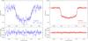 |
Fig. 1 Left plot: light curve of GJ3470b gathered with the blue channel of LBC in the Uspec band, plotted with the original sampling cadence (upper panel; the black line corresponds to the best-fit model adopted in Table 1) and residuals from the best-fit model (lower panel). Right plot: same as the left plot, but in the F972N20 band of the red channel of LBC. The two light curves are simultaneous. |
STARSKY is a photometric pipeline optimized to perform high-precision differential aperture photometry over defocused images, originally developed for the TASTE project (The Asiago Search for Transit timing variations of Exoplanets; Nascimbeni et al. 2011a,b). Its prominent feature is an empirical algorithm to choose the aperture radius and to weight the flux from the comparison stars in such a way that the off-transit scatter of the target star is minimized (Nascimbeni et al. 2013). In a second step, STARSKY searches for linear correlations between the differential magnitude and a set of standard external parameters, including the (x,y) position of the star, its FWHM, sky background, and time t. In our case, a 22.8-pixel (5.1′′) aperture was selected as the optimal one for the Uspec data set, followed by a decorrelation against FWHM and t. For the F972N20 series, the optimal aperture diameter was 40.0 pixels (9′′), followed by a decorrelation against t. It is remarkable that we did not detect any significant (x,y)-dependent systematic effect in either the blue channel or the red one, suggesting that the “extreme” defocusing strategy we applied is effective against most residual flat-field and intrapixel errors.
Summary of the best-fit parameters found for GJ3470b.
The resulting light curves are plotted in Fig. 1 in their original cadence. Their overall root mean square (RMS) scatter is 1.19 mmag (Uspec) and 0.28 mmag (F972N20) over a mean cadence of 95 s, only slightly larger than the theoretical values estimated by standard “white noise” formulae: 1.08 mmag and 0.24 mmag, respectively (Howell 2006). It is worth noting that the F972N20 series is, to our knowledge, the most precise light curve ever obtained from a ground-based facility, breaking by a narrow margin the previous record set by Tregloan-Reed & Southworth (2013) at the New Technology Telescope (NTT). The prospects from these achievements will be discussed further in Sect. 5.
4. Data analysis
4.1. Light curve modeling
The JKTEBOP code3 version 28 (Southworth et al. 2004) was employed to fit a transit model over the LBC light curves. We chose to derive the uncertainties over the best-fit parameters with a Monte Carlo bootstrap algorithm (Southworth et al. 2005), to avoid underestimation due to correlations between parameters and residual systematic noise (also called “red noise”; Pont et al. 2007). A quadratic law for modeling the stellar limb darkening (LD) is adopted (Claret 2004).
We first fitted the F972N20 curve leaving five free parameters: the radius ratio k = R⋆/Rp, the sum of the planet and star radii scaled by the orbital semi-major axis Σ = (R⋆ + Rp)/a, the orbital inclination i, the central time T0, and the linear LD coefficient u1. Following a common practice to improve the robustness of the fit (Southworth 2008), we did not fit for the quadratic LD coefficient u2, because it is strongly degenerate with u1. Even fitting for the weakly correlated parameters c1 = 2u1 + u2 and c2 = u1 − 2u2 (as suggested by Holman et al. 2006) or other linear combinations of u1 and u2 leads to unphysical results due to overfit. Instead, u2 was injected into the Monte Carlo bootstrap as a Gaussian prior, extracting its theoretical value from the tables by Claret et al. (2012), interpolated by adopting the stellar atmospheric parameters published by Demory et al. (2013) and taking their uncertainties on Teff, log g and [Fe/H] into account. As the F972N20 band is not tabulated by Claret et al. (2012), we adopted the SDSS z′ values basing on the fact that z′ and F972N20 overlap with each other in a spectral region where the specific intensity Iν(θ) is nearly devoid of spectral features (θ being the angle between the observer and the normal to the stellar surface). Moreover, for our given set of atmospheric parameters, the quadratic term u2 is nearly insensitive to λ, oscillating between 0.260 and 0.366 over the full optical-NIR range between Sloan u to 2MASS J, with a mean and RMS of 0.30 ± 0.03. After a first best-fit solution is found on real data, we ran a bootstrap analysis on 20 000 resampled light curves having the same statistical properties as the real one. The final best-fit values and the asymmetric errors on each fitted quantity were then estimated from the 50th, 15.87th, and 84.13th percentiles of the bootstrapped distribution (Table 1, second column). We emphasize that the fitted value of u1 = 0.25 ± 0.04 is perfectly consistent with the theoretical estimate u1,th = 0.275 for the z′ band by Claret et al. (2012), supporting our previous assumption u2(z′) ≃ u2(F972N20). As a further cross-check, we verified that even by setting the input u2 at the aforementioned extremal values 0.26 and 0.37, the resulting best-fit parameters change by less than 1-σ with respect to our adopted solution.
The Uspec light curve has a much lower S/N compared to the F972N20 one. We then improved the robustness of the fit by fixing the value of i (which is a purely geometrical parameter, not dependent on λ) to what was found on the F972N20 series (88.1° ± 0.3), by injecting a Gaussian distribution with the same mean and standard deviation into the bootstrap analysis. The same is done for T0. Instead, Σ (and so derived quantities such as a/R⋆) was left free, since a small dependence of these variables on λ is expected when Rp(λ) itself is not constant. The value of both u1 and u2 are fixed to their Claret et al. (2012)u′ theoretical Gaussian priors as above. The resulting best-fit values for the two fitted parameters (Σ and k) are reported in the third column of Table 1. Other quantities of interest, such as the impact parameter b and the full duration T14 (Winn et al. 2009) are extracted for both LBC light curves from the bootstrapped distribution, assuming zero eccentricity (e = 0), as suggested by the RV measurements (Bonfils et al. 2012).
We note that all the best-fit parameters we estimated on both LBC curves are in excellent agreement with each other and with the Demory et al. (2013) values (Table 1) within their errorbars. The only significant exception is k, which is offset respectively by 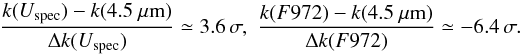 (2)This offset is not driven by a different assumption on the orbital inclination (or, equivalently, on the impact parameter), as our best-fit value is in perfect agreement with found by Demory et al. (2013) and later adopted by Fukui et al. (2013) as a prior in their analysis. As a further check, we reran our analysis, adopting a Gaussian prior and obtaining statistically indistinguishable values of k for both light curves (Δk/σ(k) ≤ 0.3). As suggested by the anonymous referee, we also redid a full analysis of both light curves by injecting Gaussian priors on c1 and c2 defined as above and leaving everything else unchanged. Again, the resulting best-fit parameters and their associated errors are fully consistent with those listed in Table 1, meaning that correlation between the LD parameters cannot explain the measured discrepancy between k(Uspec) and k(F972). In the next section we apply a correction to our k values to take the presence of unocculted starspots on the GJ3470 photosphere into account. Then in Sect. 5 we discuss the significance and origin of this chromatic signature.
The extremely high precision on T0 we achieved on the F972N20 transit (about 9 s) allowed us to compute a greatly improved orbital ephemeris of GJ3470b, by combining our measurement with the two T0 published by Demory et al. (2013) and fitting a linear ephemeris by ordinary weighted least squares: 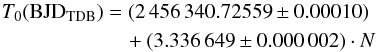 (3)where the integer epoch N is the number of transits elapsed from our LBC observation. The combination of time standard and reference frame here adopted is BJDTDB (barycentric Julian Day, barycentric dynamical time), as we follow the prescription by Eastman et al. (2010).
4.2. Correction for unocculted starspots
Starspots affect the stellar flux variations in a transit light curve in two ways. Spots that are not occulted by the planet produce a decrease in the out-of-transit flux of the star, which is the reference level to normalize the transit profile. Spots that are occulted during the transit produce a relative increase in the stellar flux because the flux blocked by the planetary disk is lower than in the case of the unperturbed photosphere. Therefore, if the star is spotted, and fo and fu are the spot filling factors of the occulted and unocculted photosphere, respectively, the relative radius of the planet ka derived from the fitting of the transit profile, is related to the true relative radius k by ![Mathematical equation: \begin{equation} k_a \simeq k \left[ 1 - \frac{1}{2} A_\lambda (\fo - \fu) \right] \textrm{ ,} \label{ratioff} \end{equation}](/articles/aa/full_html/2013/11/aa21971-13/aa21971-13-eq137.png) (4)where Aλ ≡ 1 − Fs(λ)/F⋆(λ), with F⋆(λ) and Fs(λ) the emerging fluxes from the unperturbed photosphere, and the spotted area considered as a photospheric model computed at the mean spot temperature, respectively.
(4)where Aλ ≡ 1 − Fs(λ)/F⋆(λ), with F⋆(λ) and Fs(λ) the emerging fluxes from the unperturbed photosphere, and the spotted area considered as a photospheric model computed at the mean spot temperature, respectively.
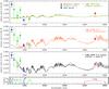 |
Fig. 2 Upper panel: reconstructed transmission spectrum of GJ3470b. The Uspec and F972N20 data points are extracted from our LBC light curves (blue circles), the g′RcIcJ points from Fukui et al. (2013) (green circles), and the 4.5 μm point from Demory et al. (2013) (red circle). The model plotted with a dark green line is scaled from a Howe & Burrows (2012) model computed for a 10-M⊕ cloud-free, haze-free planet with Teq = 700 K and a pure water (H2O) atmosphere. The open squares represent the model points integrated over the instrumental passbands. Second panel: same as above, but with a cloud-free, haze-free, metal-poor atmosphere dominated by H and He, computed by the same authors (orange line). Abundances are scaled from the solar ones (Z = 0.3 × Z⊙). Third panel: same as above, but adding the contribution of a scattering haze from Tholin particles at 1 μbar. Lower panel: instrumental passbands employed for each data point. |
Bonfils et al. (2012) suggest that GJ3470 is not a very active star according to the low projected rotational velocity (≲2 km s1) and the Hα (6562.808 Å) line observed in absorption, which are signatures of a mature star older than ~300 Myr. The same authors suggest that GJ3470 is younger than 3 Gyr, since its kinematic properties match those of the young disk population. Indeed, Fukui et al. (2013) performed a photometric monitoring of GJ3470, finding a peak-to-valley variability in the Ic band on the order of 1% in an interval of ~60 days. Assuming that such variability is due to the presence of starspots, these have a filling factor f of ~0.01 (Ballerini et al. 2012). In Eq. (4), the effects of the unocculted and occulted spots tend to compensate to each other, although the filling factor of the occulted spots may generally be higher because starspots tend to appear at low or intermediate latitudes in Sun-like stars. The filling factor of the out-of-transit spots fu can be assumed to be constant because the visibility of those spots is modulated on timescales much longer than that of the transit, i.e., on the order of the stellar rotation period, which is generally several days. Instead, the filling factor of the occulted spots fo is in general a function of the position of the center of the planetary disk along the transit chord. A variable spot distribution in the occulted area gives rise to bumps in the observed transit light curve, whereas the lack of obvious bumps in our data (Fig. 1) suggests a more or less continuous background of spots along the transit chord. In the observed case, fo can be assumed to be almost constant during the transit because otherwise we would have detected the individual spot bumps.
The maximum deviation in the relative radius k due to starspots can be computed in the unphysical hypothesis that all the spots are concentrated in the occulted area (fo = 0.01 and fu = 0) or outside the occulted area (fo = 0 and fu = 0.01). Using the grid given by Ballerini et al. (2012), where GJ3470 is very close to their case #4, the maximum correction of the relative radius in our passbands of interest is ![Mathematical equation: \begin{equation} \label{deltak} \begin{array}{lcl} \Delta k_{\max} \,(\uspec) & = & 0.00540 \\[1mm] \Delta k_{\max} \,(g') & = & 0.00538 \\[1mm] \Delta k_{\max} \,(\rc) & = & 0.00529 \\[1mm] \Delta k_{\max} \,(\ic) & = & 0.00500 \\[1mm] \Delta k_{\max} \,(F972N20) & = & 0.00500 \\[1mm] \Delta k_{\max} \,(J) & = & 0.00391 \\[1mm] \Delta k_{\max} \,(4.5\mu\mathrm{m}) & = & 0.00355 \textrm{ .}\\ \end{array} \end{equation}](/articles/aa/full_html/2013/11/aa21971-13/aa21971-13-eq157.png) (5)These corrections should be only considered an upper limit to the actual impact of activity on our estimated k(λ). For this reason, in the following discussion and plots, we adopt the uncorrected values of k(λ) and Rp(λ), unless noted otherwise, and discuss separately the limit case when Δkmax is applied.
(5)These corrections should be only considered an upper limit to the actual impact of activity on our estimated k(λ). For this reason, in the following discussion and plots, we adopt the uncorrected values of k(λ) and Rp(λ), unless noted otherwise, and discuss separately the limit case when Δkmax is applied.
A Δkmax correction ranging from 0.00355 to 0.00540 could appear quite large since it is an order of magnitude more than our best errors on k (~0.0005 in F972N20 and 4.5 μm). One has to consider, however, that the absolute scaling of this correction (which is related to the “solid” radius of the planet Rp,0 measured at H = 0) is of secondary interest for our study. Instead, the differential effect of the Δkmax correction is crucial, because it changes the slope of the Rayleigh scattering absorption and the shape of the overall transmission spectrum. It is worth noting that this may not hold when gathering transits at different epochs. In such a case, due to starspot evolution or activity cycles, the filling factors fo and fu may change, adding an unknown systematic offset between non-simultaneous measurements. However, our main result is based on simultaneous measurements (in Uspec and F972N20), so they are not affected by such an effect.
5. Discussion and conclusions
5.1. The transmission spectrum of GJ3470b
If we examine the transmission spectrum of GJ3470b as reconstructed by our LBC measurements and from those by Demory et al. (2013) and Fukui et al. (2013) (Fig. 2, large circles), it appears evident that no constant value of k could explain the data (χ2 = 67.8 for 5 degrees of freedom, corresponding to a reduced value of  ). The color dependence of k is then significant, with a steep increase toward the blue side of the spectrum, which is usually associated with scattering processes. How can we interpret this spectrum k(λ)? A detailed atmospheric modeling of GJ3470b is beyond the scope of this paper. Instead, we rescaled the model transmission spectra computed by Howe & Burrows (2012) by taking the grid point of their simulations closer to GJ3470b (Teq = 700 K, Mp = 10 M⊕) and investigating which class of atmospheric composition best matches the observed data points and which ones can be excluded.
The most striking result is that the large observed variations of k(λ) are totally incompatible with all model sets by Howe & Burrows (2012) having an atmosphere of high mean molecular weight μ, such as those made of pure H2O (Fig. 2, upper panel) or pure methane (CH4). All those models predict a very flat spectrum owing to their tiny scale height and are rejected by the available data at >10σ. The same conclusion can be drawn by considering the LBC data alone, since k(Uspec) and k(F972N20) differ by 6σ.
On the other hand, we investigated the fitness of cloud-free, haze-free atmospheric models of low μ, which is largely dominated by H and He and with a large scale height H. This is the most probable atmospheric composition expected for GJ3470b following current theories of planetary interiors (Demory et al. 2013; Rogers & Seager 2010). A metal-poor model atmosphere having a composition with Z = 0.3 × Z⊙ rescaled from a solar abundance (Howe & Burrows 2012; second panel of Fig. 2) provides us with a much better fit on the red/IR passbands (F972N20, J, 4.5 μm). Nevertheless it fails to reproduce the steep rise observed on the blue side of the spectrum, especially for our Uspec measurement. That is, the scale height required to output a Rayleigh scattering from H2 large enough to match our UV measurement would also give rise to infrared molecular features which are inconsistent with the reddest data points, in particular with the 4.5 μm one, which is in a spectral region particular sensitive to species, such as H2O and CO. Similar models, but with the addition of clouds, perform even worse, flattening the spectrum at intermediate wavelengths without significantly improving the overall quality of the fit.
An additional source of scattering, other than H2, seems to explain the data better. Fortney (2005) shows that a wide variety of condensate particles can be very efficient in this regard. Among them Tholin, for instance, is a polymer produced by UV photochemistry of CH4, said to occur on Jupiter and giant exoplanets (Sudarsky et al. 2003). Indeed, the Howe & Burrows (2012) class of models with a metal-poor H/He-dominated atmosphere and high-altitude hazes from Tholin provide us with a satisfactory fit with  (black line in Fig. 2, third panel; here the model points integrated over the instrumental passbands are plotted in magenta for clarity). Even after the maximum correction for unocculted spots (Eq. (5)) has been applied on all k(λ) points, the “haze” model with
  still fits the data set better than a flat function or any other class of Howe & Burrows (2012) models. We emphasize that Tholin was chosen here only as a test model to check whether the transmission spectrum of GJ3470b can be explained through an additional source of scattering due to condensate particles. Still, we should keep in mind that a large number of molecules are able to reproduce a similar result by means of the same physical process, and their characteristic spectral fingerprints are so subtle that they cannot be discerned in a low-resolution spectrum. Additional high S/N observations will be required to confirm this scenario, especially in the visible region at 400−900 nm (where the S/N of the Fukui et al. 2013 measurements is too low to constrain the slope of the Rayleigh scattering independently from our data) and in the near IR, for instance in the H and K spectral region, where molecular bands such as H2O, CO, or CH4 are expected to dominate the trasmission spectrum, giving rise to strong features (Fig. 2). At the estimated equilibrium temperature of GJ3470b, Teq ~ 700 K, narrow alkali metal lines, such as NaI and KI, begin to appear but are still too weak to hope in a ground-based detection, even with the current top-class facilities. Nevertheless they become very prominent at 1000 K (Fig. 6 in Howe & Burrows 2012), so searching for them could put a tight and independent upper limit to the atmospheric effective temperature of GJ3470b.
The available data can also be interpreted through a simplified analytical approach, first developed by Lecavelier des Etangs et al. (2008a) under the usual approximation of a well-mixed and isothermal atmosphere in chemical equilibrium. Following this work, we assume a scaling law of index α for the planetary cross section σ = σ0(λ/λ0)α. Under reasonable assumptions, the slope of the planetary radius as a function of wavelength λ can be expressed as a function of the scale height H (Eq. (1)) as dRp/dlnλ = αH (Lecavelier des Etangs et al. 2008a). The expression for the planetary equilibrium temperature then reduces to 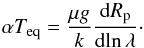 (6)If the main physical process involved is Rayleigh scattering and if we neglect atomic/molecular absorption, α = −4 and the mean molecular weight can be estimated as
 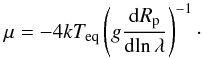 (7)We assume from Demory et al. (2013) a planetary surface gravity g = 5.75 m s-2 and an equilibrium temperature Teq = (1 − Ab)0.25(683 ± 27) K. As simple limiting cases, we can adopt two distinct values for the Bond albedo of GJ3470b: Ab = 0.3, which matches the albedo measured for Solar System icy giants (Uranus and Neptune); and Ab = 0, corresponding to a cloud-free, very dark surface as theoretically predicted for some classes of “temperate” Neptunian planets by Spiegel et al. (2010), and inferred from observations of the hot Neptune GJ436b (Cowan & Agol 2011). With these assumptions, the temperature becomes Teq = 624 ± 25 K (Ab = 0.3) and Teq = 683 ± 27 K (Ab = 0), respectively.
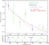 |
Fig. 3 Upper panel: same as Fig. 2, but zoomed on the optical region. The red line corresponds to the best weighted linear fit in the (lnλ,k) plane over all data points at λc < 1μm (ours and from Fukui et al. 2013) under the assumption of pure Rayleigh scattering; see text for details. Lower panel: instrumental passbands employed for each data point. |
By fitting a straight line in the (k,lnλ) plane by weighted least squares and estimating the uncertainties through an ordinary bootstrap algorithm we find  (8)which is equivalent to dRp/dlnλ ≃ − 3000 ± 500 km for both cases once we adopt R⋆ = 0.568 R⊙ as the stellar radius from Demory et al. (2013) and propagate the uncertainties. From Eq. (7), and taking the errors on all variables into account, we derive a mean molecular weight of
  atomic mass units (amu; Ab = 0.3) or
  amu (Ab = 0) for GJ3470b, that is, a mean molecular weight consistent with that of a H/He-dominated atmosphere with subsolar chemical abundances. The error bars are largely dominated by the uncertainty on k. Our result is virtually independent of the correction Δkmax in Eq. (5), which leads to a nearly unchanged μ = 1.3 ± 0.25 amu (Ab = 0.3) when it is applied. We emphasize however that the last approach does not take into account that the k value at 4.5 μm seems to be inconsistent with a cloud-free H/He envelope. On the other hand, the (k,lnλ) fit also demonstrates that the increase in k (or Rp) at blue wavelengths is significant at 5.8σ, regardless of the underlying physical process. The significance is largely driven by our Uspec point, and this emphasizes the importance of the optical UV bands in exoatmospheric studies.
 |
Fig. 4 Upper panel: synthetic 1-R⊕ transit (black line) injected in the residuals of our F972N20 light curve (red points and error bars), showing that a short-period Earth around an M1.5V star would have been detectable from our photometry. Lower panel: same as above, binned over 20-min intervals. |
5.2. Pushing the limits of ground-based photometry
As a final note we highlight that the accuracy of our F972N20 light curve is close to the theoretical limit expected for a photometric series gathered with a 8.4-m telescope. It is interesting to investigate the consequences of this unprecedented accuracy on the ground-based detection of very small planets. A way to do it is to extract the F972N20 residuals from our best-fit model and to inject on them a synthetic transit corresponding to a 1-R⊕ planet hosted by a star having the same radius of GJ3470, i.e. a M1.5V dwarf. Having employed real residuals to perform this simulation, we are confident that the instrumental, atmospheric, and astrophysical noise contributions are preserved. The result is plotted in Fig. 4, with the original 90-s sampling rate (upper panel) and binned over 20-min intervals to increase the S/N (lower panel). The transit signature is clearly detectable with high confidence (9σ), opening up new prospects for a future targeted search for short-period, Earth-sized transiting planets around M dwarfs without necessarily resorting to much more expensive, dedicated space missions.
The short-term photometric accuracy of the data presented here is probably not achievable on a longer term (night-to-night) baseline, owing to atmospheric and instrumental systematic drifts. This limitation, combined with the extremely low density of bright M dwarfs in the sky, prevents us from a “classical” transit search of terrestrial planets with a camera such as LBC. However, when a sample of low-mass planets hosted by red dwarfs and discovered by an RV survey is available, it will be possible to predict the instant of the inferior conjunction within a few hours of uncertainty and to search for planetary transits in that observational window. For a scaled-down version of GJ3470b, the a priori transit probability is around 8%, meaning that at least a dozen RV planets need to be followed up in order to detect one transit. Given the importance of these planets for the exoplanetary studies, thanks especially to their closeness to the habitable zone and to the relatively easy access to their atmospheric signatures, we suggest that a targeted search would be worth implementation.
Note added in proof. Simultaneously with this report, an analysis of optical and infrared transit photometry of GJ 3470b was released that also suggests a hazy atmosphere (Crossfield et al. 2013).
According to exoplanets.org (Wright et al. 2011).
The FHWM of the F972N20 band is 22 nm; the passbands of both filters are tabulated in http://abell.as.arizona.edu/~{}lbtsci/ Instruments/LBC/lbc_description.html#filters.html and plotted in the bottom panels of Figs. 2 and 3.
Acknowledgments
This work was partially supported by PRIN INAF 2008 “Environmental effects in the formation and evolution of extrasolar planetary system”. V.N. and G.P. acknowledge partial support by the Università di Padova through the “progetto di Ateneo #CPDA103591”. V.N. acknowledges partial support from INAF-OAPd through the grant “Analysis of HARPS-N data in the framework of GAPS project” (#19/2013). Some tasks of our data analysis have been carried out with the VARTOOLS (Hartman et al. 2008) and Astrometry.net codes (Lang et al. 2010). This research made use of the International Variable Star Index (VSX) database, operated at AAVSO, Cambridge, Massachusetts, USA.
References
- Adams, E. R., Seager, S., & Elkins-Tanton, L. 2008, ApJ, 673, 1160 [NASA ADS] [CrossRef] [Google Scholar]
- Baglin, A., Auvergne, M., Barge, P., et al. 2006, in ESA SP, eds. M. Fridlund, A. Baglin, J. Lochard, & L. Conroy, 1306, 33 [Google Scholar]
- Ballerini, P., Micela, G., Lanza, A. F., & Pagano, I. 2012, A&A, 539, A140 [NASA ADS] [CrossRef] [EDP Sciences] [Google Scholar]
- Batalha, N. M., Borucki, W. J., Bryson, S. T., et al. 2011, ApJ, 729, 27 [NASA ADS] [CrossRef] [Google Scholar]
- Bonfils, X., Gillon, M., Udry, S., et al. 2012, A&A, 546, A27 [NASA ADS] [CrossRef] [EDP Sciences] [Google Scholar]
- Borucki, W. J., Koch, D., Basri, G., et al. 2010, Science, 327, 977 [NASA ADS] [CrossRef] [PubMed] [Google Scholar]
- Charbonneau, D., Berta, Z. K., Irwin, J., et al. 2009, Nature, 462, 891 [NASA ADS] [CrossRef] [PubMed] [Google Scholar]
- Claret, A. 2004, A&A, 428, 1001 [NASA ADS] [CrossRef] [EDP Sciences] [Google Scholar]
- Claret, A., Hauschildt, P. H., & Witte, S. 2012, A&A, 546, A14 [NASA ADS] [CrossRef] [EDP Sciences] [Google Scholar]
- Cochran, W. D., Fabrycky, D. C., Torres, G., et al. 2011, ApJS, 197, 7 [NASA ADS] [CrossRef] [Google Scholar]
- Cowan, N. B., & Agol, E. 2011, ApJ, 729, 54 [NASA ADS] [CrossRef] [Google Scholar]
- Crossfield, I. J. M., Barman, T., Hansen, B. M. S., & Howard, A. W. 2013, A&A, in press, DOI: 10.1051/0004-6361/201322278 [Google Scholar]
- de Mooij, E. J. W., Brogi, M., de Kok, R. J., et al. 2012, A&A, 538, A46 [NASA ADS] [CrossRef] [EDP Sciences] [Google Scholar]
- Demory, B.-O., Torres, G., Neves, V., et al. 2013, ApJ, 768, 154 [NASA ADS] [CrossRef] [Google Scholar]
- Eastman, J., Siverd, R., & Gaudi, B. S. 2010, PASP, 122, 935 [NASA ADS] [CrossRef] [Google Scholar]
- Fortney, J. J. 2005, MNRAS, 364, 649 [NASA ADS] [CrossRef] [Google Scholar]
- Fukui, A., Narita, N., Kurosaki, K., et al. 2013, ApJ, 770, 95 [NASA ADS] [CrossRef] [Google Scholar]
- Giallongo, E., Ragazzoni, R., Grazian, A., et al. 2008, A&A, 482, 349 [NASA ADS] [CrossRef] [EDP Sciences] [Google Scholar]
- Haghighipour, N. 2011, Contemporary Phys., 52, 403 [NASA ADS] [CrossRef] [Google Scholar]
- Hartman, J. D., Gaudi, B. S., Holman, M. J., et al. 2008, ApJ, 675, 1254 [NASA ADS] [CrossRef] [Google Scholar]
- Hartman, J. D., Bakos, G. Á., Kipping, D. M., et al. 2011, ApJ, 728, 138 [NASA ADS] [CrossRef] [Google Scholar]
- Holman, M. J., Winn, J. N., Latham, D. W., et al. 2006, ApJ, 652, 1715 [NASA ADS] [CrossRef] [Google Scholar]
- Howe, A. R., & Burrows, A. S. 2012, ApJ, 756, 176 [NASA ADS] [CrossRef] [Google Scholar]
- Howell, S. B. 2006, Handbook of CCD astronomy, eds. R. Ellis, J. Huchra, S. Kahn, G. Rieke, & P. B. Stetson (Cambridge University Press) [Google Scholar]
- Lang, D., Hogg, D. W., Mierle, K., Blanton, M., & Roweis, S. 2010, AJ, 139, 1782 [Google Scholar]
- Lecavelier des Etangs, A., Pont, F., Vidal-Madjar, A., & Sing, D. 2008a, A&A, 481, L83 [NASA ADS] [CrossRef] [Google Scholar]
- Lecavelier des Etangs, A., Vidal-Madjar, A., Désert, J.-M., & Sing, D. 2008b, A&A, 485, 865 [NASA ADS] [CrossRef] [EDP Sciences] [Google Scholar]
- Nascimbeni, V., Piotto, G., Bedin, L. R., & Damasso, M. 2011a, A&A, 527, A85 [NASA ADS] [CrossRef] [EDP Sciences] [Google Scholar]
- Nascimbeni, V., Piotto, G., Bedin, L. R., et al. 2011b, A&A, 532, A24 [NASA ADS] [CrossRef] [EDP Sciences] [Google Scholar]
- Nascimbeni, V., Cunial, A., Murabito, S., et al. 2013, A&A, 549, A30 [NASA ADS] [CrossRef] [EDP Sciences] [Google Scholar]
- Pont, F., Gilliland, R. L., Moutou, C., et al. 2007, A&A, 476, 1347 [NASA ADS] [CrossRef] [EDP Sciences] [MathSciNet] [Google Scholar]
- Rogers, L. A., & Seager, S. 2010, ApJ, 716, 1208 [NASA ADS] [CrossRef] [Google Scholar]
- Seager, S., & Deming, D. 2010, ARA&A, 48, 631 [NASA ADS] [CrossRef] [Google Scholar]
- Sing, D. K., Pont, F., Aigrain, S., et al. 2011, MNRAS, 416, 1443 [NASA ADS] [CrossRef] [Google Scholar]
- Southworth, J. 2008, MNRAS, 386, 1644 [NASA ADS] [CrossRef] [Google Scholar]
- Southworth, J., Maxted, P. F. L., & Smalley, B. 2004, MNRAS, 351, 1277 [NASA ADS] [CrossRef] [Google Scholar]
- Southworth, J., Smalley, B., Maxted, P. F. L., Claret, A., & Etzel, P. B. 2005, MNRAS, 363, 529 [NASA ADS] [CrossRef] [Google Scholar]
- Spiegel, D. S., Burrows, A., Ibgui, L., Hubeny, I., & Milsom, J. A. 2010, ApJ, 709, 149 [NASA ADS] [CrossRef] [Google Scholar]
- Sudarsky, D., Burrows, A., & Hubeny, I. 2003, ApJ, 588, 1121 [NASA ADS] [CrossRef] [Google Scholar]
- Tregloan-Reed, J., & Southworth, J. 2013, MNRAS, 431, 966 [NASA ADS] [CrossRef] [Google Scholar]
- Winn, J. N., Holman, M. J., Carter, J. A., et al. 2009, AJ, 137, 3826 [NASA ADS] [CrossRef] [Google Scholar]
- Wright, J. T., Fakhouri, O., Marcy, G. W., et al. 2011, PASP, 123, 412 [NASA ADS] [CrossRef] [Google Scholar]
- Zhou, J.-L., Xie, J.-W., Liu, H.-G., Zhang, H., & Sun, Y.-S. 2012, RA&A, 12, 1081 [Google Scholar]
All Tables
All Figures
|
Fig. 1 Left plot: light curve of GJ3470b gathered with the blue channel of LBC in the Uspec band, plotted with the original sampling cadence (upper panel; the black line corresponds to the best-fit model adopted in Table 1) and residuals from the best-fit model (lower panel). Right plot: same as the left plot, but in the F972N20 band of the red channel of LBC. The two light curves are simultaneous. |
| In the text | |
|
Fig. 2 Upper panel: reconstructed transmission spectrum of GJ3470b. The Uspec and F972N20 data points are extracted from our LBC light curves (blue circles), the g′RcIcJ points from Fukui et al. (2013) (green circles), and the 4.5 μm point from Demory et al. (2013) (red circle). The model plotted with a dark green line is scaled from a Howe & Burrows (2012) model computed for a 10-M⊕ cloud-free, haze-free planet with Teq = 700 K and a pure water (H2O) atmosphere. The open squares represent the model points integrated over the instrumental passbands. Second panel: same as above, but with a cloud-free, haze-free, metal-poor atmosphere dominated by H and He, computed by the same authors (orange line). Abundances are scaled from the solar ones (Z = 0.3 × Z⊙). Third panel: same as above, but adding the contribution of a scattering haze from Tholin particles at 1 μbar. Lower panel: instrumental passbands employed for each data point. |
| In the text | |
|
Fig. 3 Upper panel: same as Fig. 2, but zoomed on the optical region. The red line corresponds to the best weighted linear fit in the (lnλ,k) plane over all data points at λc < 1μm (ours and from Fukui et al. 2013) under the assumption of pure Rayleigh scattering; see text for details. Lower panel: instrumental passbands employed for each data point. |
| In the text | |
|
Fig. 4 Upper panel: synthetic 1-R⊕ transit (black line) injected in the residuals of our F972N20 light curve (red points and error bars), showing that a short-period Earth around an M1.5V star would have been detectable from our photometry. Lower panel: same as above, binned over 20-min intervals. |
| In the text | |
Current usage metrics show cumulative count of Article Views (full-text article views including HTML views, PDF and ePub downloads, according to the available data) and Abstracts Views on Vision4Press platform.
Data correspond to usage on the plateform after 2015. The current usage metrics is available 48-96 hours after online publication and is updated daily on week days.
Initial download of the metrics may take a while.