| Issue |
A&A
Volume 559, November 2013
|
|
|---|---|---|
| Article Number | A64 | |
| Number of page(s) | 8 | |
| Section | Astrophysical processes | |
| DOI | https://doi.org/10.1051/0004-6361/201321963 | |
| Published online | 15 November 2013 | |
Revisiting the formation rate and redshift distribution of long gamma-ray bursts
1
University of Nice-Sophia Antipolis – Observatoire de la Côte
d’Azur
06304
Nice
France
e-mail: kanaan@oca.eu; pacheco@oca.eu
2
Laboratoire Lagrange, UMR 7293, BP 4229, 06304
Nice Cedex 4,
France
Received:
25
May
2013
Accepted:
5
September
2013
Using a novel approach, the distribution of fluences of long gamma-ray bursts derived from the Swift-BAT catalog was reproduced by a jet-model characterized by the distribution of the total radiated energy in γ-rays and the distribution of the aperture angle of the emission cone. The best fit between simulated and observed fluence distributions permits one to estimate the parameters of the model. An evolution of the median energy of the bursts is required to adequately reproduce the observed redshift distribution of the events when the formation rate of γ-ray bursts follows the cosmic star formation rate. For our preferred model, the median jet energy evolves as EJ ∝ e0.5(1 + z) and the mean expected jet energy is 3.0 × 1049 erg, which agrees with the mean value derived from afterglow data. The estimated local formation rate is Rgrb = 290 Gpc-3 yr-1, representing less than 9% of the local formation rate of type Ibc supernovae. This result also suggests that the progenitors of long gamma-ray bursts have masses ≥ 90 M⊙ when a Miller-Scalo initial mass function is assumed.
Key words: gamma-ray burst: general
© ESO, 2013
1. Introduction
Gamma-ray bursts (GRBs) are among the most violent and energetic phenomena observed in the Universe. The total energy emitted (if isotropically) in the form of energetic photons can attain values of up to few times 1054 erg, two orders of magnitude higher than the energy released by supernova explosions. However, this dramatic energy output can be considerably alleviated if the emission is strongly collimated along jets (Rhoads 1999).
GRBs are classified into two main classes: long (LGRB) and short (SGRB) (Kouveliotou et al. 1993), according to the observed burst duration. The first category includes events with durations longer than ~2 s, while the second includes those with durations shorter than ~2 s. More recent investigations indicate that there may be an intermediate class of bursts that has the softest energy spectra of the three (Horváth et al. 2008, 2010; Huja et al. 2009). The comparison between Swift and BATSE samples indicates that the population fraction in these classes differs because Swift detectors are more sensitive to soft and weak bursts. As a consequence, the probability detection of bursts included in the intermediate group is enhanced compared with the BATSE results (Horváth et al. 2010). Considering only the more conservative classification into two categories, Swift data indicate that 83% of the events are LGRBs, while only 17% are included in the SGRB class (Huja et al. 2009). It is worth mentioning that these two classes have indeed some distinct properties, which are examined below.
For instance, in the plane defined by the temporal lag between features in the light curve observed at different wavelengths and the peak luminosity, these two aforementioned classes are clearly distributed separately. Moreover, there are other indications that LGRBs and SGRBs represent events with different origins. LGRBs are generally located in active star formation regions preferentially found in low-metallicity and low-luminosity galaxies (Fruchter et al. 2006). These events might be related with type Ibc supernovae because several unambiguous spectroscopic identifications were obtained up to now (Stanek et al. 2003; Hjorth et al. 2003; Woosley & Bloom 2006; Berger et al. 2011). However, late radio observations of 68 SNIbc, searching for emission attributable to off-axis events, indicate that less than 10% of type Ibc supernovae might be related to LGRBs (Soderberg et al. 2006b). Recent Swift data indicate that SGRBs occur in galaxies with different morphologies, including early-type objects in which no star formation activity is observed (Berger 2011; Church et al. 2011). Moreover the positioning of these bursts indicates a wide range of spatial offsets from the (assumed) host galaxy (Church et al. 2011). This would be expected if SGRBs were the consequence of a merger of two compact objects that have received a kick velocity during their formation (Church et al. 2011). Moreover, as mentioned above, in addition to the possible existence of an intermediate class, some authors have suggested two other subclasses: subluminous long GRBs (SL-LGRBs) and short GRBs with extended emission (SGRB-EE; Coward 2005; Murase et al. 2006; Guetta & Della Valle 2007; Imerito et al. 2008). But, possible criticisms not withstanding these subclasses are ignored in our investigation and only LGRBs are considered. If LGRBs are the consequence of the death of massive stars, their formation rate Rgrb as a function of the redshift is expected to be proportional to the cosmic star formation rate (CSFR) R∗(z). The observed rate of LGRBs, which permits estimating the local formation rate, will depend not only on the CSFR, but also on the luminosity function φ(L). According to Salvaterra & Chincarini (2007), models in which LGRBs trace the CSFR and are described by a non-evolving luminosity function underestimate the number of events at high redshift. This difficulty could be surpassed if the luminosity function evolves in the sense that LGRBs are more luminous at high redshift (Butler et al. 2010). Including a moderate evolution in the luminosity function and considering an isotropic emission model, Salvaterra & Chincarini (2007) derived a local LGRB formation rate Rgrb = 0.12 Gpc-3 yr-1, while more recently, Salvaterra et al. (2011) argued that a strong evolution of the luminosity function is required to explain the redshift distribution of these events. A different method was adopted by Wanderman & Piran (2010), who derived the luminosity function and the local formation rate by directly inverting the redshift distribution of LGRBs. They estimated a local rate Rgrb = 1.3 Gpc-3 yr-1, increasing up to z ~ 3 and decreasing for high redshift. Another possibility that could explain the excess of events at high redshift is to assume that the efficiency of massive stars of forming GRBs increases with redshift. A variable efficiency of forming GRBs could be an effect due to the metallicity of the environment (Daigne et al. 2006; Salvaterra & Chincarini 2007; Qin et al. 2010; Cao et al. 2011; Virgili et al. 2011). If one accepts that LGRBs are formed preferentially in a metal-poor medium, the association of (at least a fraction of them) with type Ibc supernovae is difficult to understand since SNIbc preferentially occur in galaxies with high metallicity (Prantzos & Boissier 2003; Prieto et al. 2008). Pélangeon et al. (2008) followed a different approach to estimate the local formation rate of GRBs. They calculated the volume detectability for sources listed in the HETE-2 catalog, that is the volume Vmax of the Universe in which events are bright enough to be included in their sample. Then, the number of GRBs inside Vmax was calculated, which permits an estimate of Rgrb. They obtained, before correcting for beaming, a local formation rate Rgrb ~ 11 Gpc-3 yr-1, a value substantially higher than the estimates mentioned previously.
In the present work a novel approach was adopted to derive the local formation rate of LGRBs and the redshift distribution of these events. A Monte Carlo code was developed to estimate the probability that a GRB generated at a given redshift is detected in a given energy band of the detector (visibility function) which in our case corresponds to the Swift-BAT experiment. Once the visibility function is known, the formation rate and the redshift distribution of GRBs can be estimated. Another particular aspect of our approach is that instead of introducing the luminosity function of GRBs as is commonly done, we consider the energy distribution of the events, that is the probability for a given burst to occur with an energy E. The best parameters defining the assumed energy distribution were then determined by comparing predicted fluences with those given by the Swift-BAT catalog. The choice of fluences is dictated by the fact that this primary physical quantity is well defined and well measured. The paper is organized as follows: in Sect. 2 the jet model and the Monte Carlo code are described; in Sect. 3 we discuss the simulations and the data analysis that lead to an estimate of the parameters that define the energy distribution; in Sect. 4 the main results are given, and finally we present the conclusions in Sect. 5.
2. Model and the Monte Carlo code
Two phenomenological jet models have been intensively discussed in the literature. The so-called universal model, in which jets have the same structure but the angular energy distribution varies (Meszaros et al. 1999; Rossi et al. 2002) and the alternative model, which considers that the angular energy distribution is uniform inside the jet, but the total emitted energy is nearly the same for all events, although beamed into different opening angles (Rhoads 1997; Dai & Cheng 2001; Frail et al. 2001).
In our approach, we assumed that the γ-ray emission occurs along two cones
of aperture 2θ. In this case, the total energy
EJ emitted along the jets is related to the isotropic energy
Eiso by the well-known relation  (1)We assumed furthermore that
the probability for an event to occur with an energy EJ is given
by a log-normal distribution, that is
(1)We assumed furthermore that
the probability for an event to occur with an energy EJ is given
by a log-normal distribution, that is ![\begin{equation} \label{distributionEJ} P(E_{\rm J}){\rm d}\ln E_{\rm J} = A\exp\left[-\frac{\left(\ln E_{\rm J}-\ln E_{\rm med}\right)^2}{2\sigma^2_{\ln E_{\rm j}}}\right]{\rm d}\ln E_{\rm J} , \end{equation}](/articles/aa/full_html/2013/11/aa21963-13/aa21963-13-eq22.png) (2)where
A is a normalization constant. The median,
lnEmed, and the dispersion,
σlnEJ, of the log-normal
distribution are free parameters to be determined. These parameters are constants if there
is no evolution in the energy distribution. Since this possibility cannot be excluded, cases
in which the median energy evolves were also considered and were modeled simply by the
relation
(2)where
A is a normalization constant. The median,
lnEmed, and the dispersion,
σlnEJ, of the log-normal
distribution are free parameters to be determined. These parameters are constants if there
is no evolution in the energy distribution. Since this possibility cannot be excluded, cases
in which the median energy evolves were also considered and were modeled simply by the
relation  (3)where
lnEo and δ are constants
(note that the median energy of the distribution at z = 0 is
Emed(0) = Eoeδ).
The assumption that at high redshift LGRBs might be more energetic may be justified by the
following argument. If jets are related to the rotation of the GRB progenitor, it is
expected that in the past, massive stars were formed preferentially in a metal-poor
environment and, consequently, these stars have mass-loss rates lower than stars formed in
metal-rich regions. Less massive axisymmetric winds carry out less angular momentum (de Araujo & de Freitas Pacheco 1994; de Araujo et al. 1994). In this case, the progenitors of
LGRBs formed in a metal-poor environment are expected to have higher rotation rates and to
produce stronger jets. Note that in this context the metallicity is expected to affect the
energetics of the event, but not necessarily the formation efficiency. We cannot exclude the
possibility that both the efficiency to produce GRBs and the energy (or luminosity)
distribution vary with redshift, but in this investigation we considered a constant
efficiency per unit of stellar mass formed and possible evolutionary effects only in the
energy distribution, as modeled by Eq. (3).
(3)where
lnEo and δ are constants
(note that the median energy of the distribution at z = 0 is
Emed(0) = Eoeδ).
The assumption that at high redshift LGRBs might be more energetic may be justified by the
following argument. If jets are related to the rotation of the GRB progenitor, it is
expected that in the past, massive stars were formed preferentially in a metal-poor
environment and, consequently, these stars have mass-loss rates lower than stars formed in
metal-rich regions. Less massive axisymmetric winds carry out less angular momentum (de Araujo & de Freitas Pacheco 1994; de Araujo et al. 1994). In this case, the progenitors of
LGRBs formed in a metal-poor environment are expected to have higher rotation rates and to
produce stronger jets. Note that in this context the metallicity is expected to affect the
energetics of the event, but not necessarily the formation efficiency. We cannot exclude the
possibility that both the efficiency to produce GRBs and the energy (or luminosity)
distribution vary with redshift, but in this investigation we considered a constant
efficiency per unit of stellar mass formed and possible evolutionary effects only in the
energy distribution, as modeled by Eq. (3).
We assumed also that the probability G(θ) for having a
jet with an opening half-angle θ is independent of the jet energy. In other
words, the probabilities P(EJ) and
G(θ) are statistically independent. The observed
distribution of opening angles Q(θ) is related to the
intrinsic distribution by the relation  (4)where we used the fact that
the probability for the jet with an opening half-angle θ to be aligned with
the line of sight is (1−cosθ). From Eq. (4) the intrinsic distribution G(θ) can
be derived if the observed distribution Q(θ) is known.
(4)where we used the fact that
the probability for the jet with an opening half-angle θ to be aligned with
the line of sight is (1−cosθ). From Eq. (4) the intrinsic distribution G(θ) can
be derived if the observed distribution Q(θ) is known.
Estimates of the opening angle of the jet depend on the model parameters. Racusin et al. (2009) computed opening angles for 28 GRBS
based on the analysis of the break time of the conical blast wave describing X-ray
afterglows. A large sample was considered by Goldstein et
al. (2011), who used the Ghirlanda lower limit (Ghirlanda et al. 2004) in the plane εpeak − fluence,
calibrated with GRBs that have well-constrained jet opening angles. These studies suggest
that the observed distribution of values of θ can be represented by a
log-normal distribution. Although this may be only a consequence of the assumptions made for
estimating θ, we adopted this in our computations, that is ![\begin{equation} \label{goldstein} Q(\theta){\rm d}\ln\theta=\frac{1}{\sqrt{2\pi\sigma^2}}\exp\left[-\frac{\left(\ln\theta-\ln\theta_{\rm med}\right)^2}{2\sigma^2}\right] {\rm d}\ln\theta . \end{equation}](/articles/aa/full_html/2013/11/aa21963-13/aa21963-13-eq38.png) (5)Our preferred model has
an observed median value for the jet opening angle
2θmed = 16° and a dispersion
σ = 0.76. It should be mentioned that recently Lu et al. (2012) claimed that the opening angles are anti-correlated with
the redshift, meaning that jets were narrower at high z. This possibility
is not considered here although it deserves more detailed investigation.
(5)Our preferred model has
an observed median value for the jet opening angle
2θmed = 16° and a dispersion
σ = 0.76. It should be mentioned that recently Lu et al. (2012) claimed that the opening angles are anti-correlated with
the redshift, meaning that jets were narrower at high z. This possibility
is not considered here although it deserves more detailed investigation.
2.1. Code
Our code is similar to that developed by Lamb et al. (2005), who aimed to investigate the unified jet model. For the sake of completeness, we present here the main steps defining the sequence of calculations that permitted us to produce a mock catalog of LGRBs, from which one can identify the differences between the present approach and that of the aforementioned authors.
-
1)
Initially, the redshift of the object is determined by a probability function proportional to the CSFR. The adopted CSFR was parametrized by the usual form proposed by Cole et al. (2001), that is
![\begin{equation} \label{csfr} R_*(z)=h_{70}\frac{(a+bz)}{\left[1+(z/c)^{\rm d}\right]} , \end{equation}](/articles/aa/full_html/2013/11/aa21963-13/aa21963-13-eq42.png) (6)where
a = 0.0103, b = 0.12, c = 5.0,
d = 2.8, with the CSFR given in
M⊙ Mpc-3 yr-1.
h70 is the Hubble parameter in units of 70
km s-1 Mpc-1. This expression provides a quite good fit of
the existing data (see, for instance, Hopkins
& Beacom 2006) and is consistent with the cosmological simulations
by Filloux et al. (2010, 2011). Under these conditions, the probability
Ψ(z) of generating a burst in the redshift interval
z,z + dz is
(6)where
a = 0.0103, b = 0.12, c = 5.0,
d = 2.8, with the CSFR given in
M⊙ Mpc-3 yr-1.
h70 is the Hubble parameter in units of 70
km s-1 Mpc-1. This expression provides a quite good fit of
the existing data (see, for instance, Hopkins
& Beacom 2006) and is consistent with the cosmological simulations
by Filloux et al. (2010, 2011). Under these conditions, the probability
Ψ(z) of generating a burst in the redshift interval
z,z + dz is
 (7)where
dV is the comoving volume differential element and the
normalization constant is defined by
(7)where
dV is the comoving volume differential element and the
normalization constant is defined by
 (8)where we
assumed zmax = 15, but the results are not significantly
modified for higher values. After obtaining the redshift z from the
probability function Ψ(z), the luminosity distance
DL is computed from the adopted
cosmology which, in our case, was a ΛCDM model defined by the parameters
H0 = 70 km s-1 Mpc-1,
Ωm = 0.3 and Ωv = 0.7.
(8)where we
assumed zmax = 15, but the results are not significantly
modified for higher values. After obtaining the redshift z from the
probability function Ψ(z), the luminosity distance
DL is computed from the adopted
cosmology which, in our case, was a ΛCDM model defined by the parameters
H0 = 70 km s-1 Mpc-1,
Ωm = 0.3 and Ωv = 0.7. -
2)
In a second step, the energy of the jet is obtained by using the probability function P(EJ) for given values of the median and the dispersion, according to cases including or excluding the evolution of the burst mean energy.
-
3)
The opening angle of the jet was derived from the probability function G(θ) as described previously.
-
4)
In the next step, we determine whether the jet points in the direction of the observer with a probability (1−cosθ). If the jet is not visible, the event is saved with its corresponding redshift as an unseen burst. If the event occurs in the observer’s direction, we still have to verify whether the resulting photon rate in the observer’s frame will be able to trigger the considered detector.
-
5)
We assumed that the photon energy distribution of the burst can be represented by a Band function (Band et al. 1993) with exponents α = −1.0 and β = −2.25, typical values found from fits of existing data. In this case, for photon energies ε ≤ 1.25εpeak the photon spectrum is
 (9)where
K is a normalization constant. For photon energies
ε > 1.25εpeak
the photon energy distribution is
(9)where
K is a normalization constant. For photon energies
ε > 1.25εpeak
the photon energy distribution is
 (10)In these relations
εpeak is the energy at which the function
ε2B(ε) attains a
maximum. The value of εpeak for a given simulated event
was estimated from the so-called Amati relation, which correlates
εpeak with the equivalent isotropic energy of the
burst. In our simulations Eiso was estimated from Eq.
(1), using EJ obtained in step (2). From data by Amati et al. (2008, 2009) the following fit was obtained and adopted for our simulations (rest
frame quantities):
(10)In these relations
εpeak is the energy at which the function
ε2B(ε) attains a
maximum. The value of εpeak for a given simulated event
was estimated from the so-called Amati relation, which correlates
εpeak with the equivalent isotropic energy of the
burst. In our simulations Eiso was estimated from Eq.
(1), using EJ obtained in step (2). From data by Amati et al. (2008, 2009) the following fit was obtained and adopted for our simulations (rest
frame quantities):  (11)where
Eiso is in erg and εpeak
is in keV.
(11)where
Eiso is in erg and εpeak
is in keV. -
6)
According to Band (2006), detectable events must have a photon flux above the threshold value CT of the detector. Band (2006) computed this threshold for different experiments, in particular for Swift’s BAT, whose data we used here. The sensitivity was computed in the 1−1000 keV band as a function of the peak energy at the observer’s frame (
 ), taking
into account the photon distribution in the considered energy interval. To
facilitate the computations, the sensitivity
), taking
into account the photon distribution in the considered energy interval. To
facilitate the computations, the sensitivity  was fitted by the
polynomial
was fitted by the
polynomial  (12)where
 . In this
equation the peak energy is given in keV and the photon flux
CT is given in
ph cm-2 s-1.
. In this
equation the peak energy is given in keV and the photon flux
CT is given in
ph cm-2 s-1.
To verify whether a
given simulated burst triggers the detector, its average photon flux in the 1−1000 keV
band was estimated by the following procedure. First, a sample including 133 LGRB with
measured T90 (duration in which 90% of the total burst fluence
is detected) was prepared. After correcting for the rest frame, the resulting distribution
 was fitted by a log-normal
distribution characterized by a median
was fitted by a log-normal
distribution characterized by a median  and
a dispersion
and
a dispersion  . The distribution
permits one to assign the
duration (in the rest frame) of the considered event, via a Monte Carlo procedure. In this
case, the expected photon rate Rγ
corresponding to this simulated event in the observer’s frame is
. The distribution
permits one to assign the
duration (in the rest frame) of the considered event, via a Monte Carlo procedure. In this
case, the expected photon rate Rγ
corresponding to this simulated event in the observer’s frame is  (13)Note that in this
equation there is no (1 + z) term in the denominator since it cancels
with a similar term in the numerator due to the jet energy, which is also referred to the
rest frame. The term
S(ε1,ε2)
is computed from the equation
(13)Note that in this
equation there is no (1 + z) term in the denominator since it cancels
with a similar term in the numerator due to the jet energy, which is also referred to the
rest frame. The term
S(ε1,ε2)
is computed from the equation 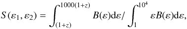 (14)which represents the
fraction of the total photons released in the event and detected in the range 1−1000
keV. Note that the limits of the integral are corrected for the rest frame and the total
energy released in the event is assumed to be restricted to the normalization interval 1
keV−10 MeV. Under these conditions, detectable events satisfy the condition
Rγ(εpeak) ≥ CT(εpeak)
and are saved as such. It is worth mentioning that although our detection condition refers
to the average flux of the event, the BAT detector triggers the burst with respect to the
peak flux, which is higher. In practice, this affects the estimate of the visibility
function, as we see below. To compute peak fluxes a model for the burst time profile is
required, which is currently not included in our code. The diversity of time profiles
makes this modeling difficult, but this problem is under investigation and will be the
subject of a future paper.
(14)which represents the
fraction of the total photons released in the event and detected in the range 1−1000
keV. Note that the limits of the integral are corrected for the rest frame and the total
energy released in the event is assumed to be restricted to the normalization interval 1
keV−10 MeV. Under these conditions, detectable events satisfy the condition
Rγ(εpeak) ≥ CT(εpeak)
and are saved as such. It is worth mentioning that although our detection condition refers
to the average flux of the event, the BAT detector triggers the burst with respect to the
peak flux, which is higher. In practice, this affects the estimate of the visibility
function, as we see below. To compute peak fluxes a model for the burst time profile is
required, which is currently not included in our code. The diversity of time profiles
makes this modeling difficult, but this problem is under investigation and will be the
subject of a future paper.
3. Simulations and data analysis
For each pair of the parameters characterizing the log-normal distributions of the jet energy and of the opening half-angle of the jet, that is the median and the dispersion, a series of runs were performed until the number of detected events was equal to 105. The total number of runs required to satisfy this condition depends on the adopted emission model. For isotropic emission, the total number is of the order on 2 × 10⁶, while in the case of beamed emission, the number is considerably higher, on order of 7 × 10⁸.
The detected events constitute a catalog, including parameters as the redshift
z, the jet energy EJ, the opening half-angle
θ of the jet and the peak energy εpeak,
characterizing the hardness (or softness) of the photon spectrum. All these parameters
permit one to compute the expected fluences in the Swift energy bands 15−25
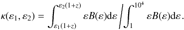
keV, 25−50 keV, 50−100 keV, 100−150 keV, and 15−150 keV by the equation 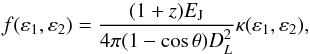 (15)where the fraction of the
bolometric energy in a given band
(ε1 − ε2) is
(15)where the fraction of the
bolometric energy in a given band
(ε1 − ε2) is
 (16)After computing the
fluences, they are distributed in logarithmic bins
(Δlog f(εi,εi + 1) = 0.20)
and their frequency distribution is computed. The simulated fluence frequency distribution
in different energy bands is then compared with those derived from data of the second
Swift-BAT catalog (Sakamoto et al.
2011). From the 475 events present in the catalog, we prepared a culled sample of
403 objects, discarding events with
T90 < 2 s and those without fluence
data on all the considered energy bands. Of the excluded events, 49 have short duration, 19
have incomplete data, and 4 have an uncertain classification. The quality of the fit was
measured by the χ2 test, namely
(16)After computing the
fluences, they are distributed in logarithmic bins
(Δlog f(εi,εi + 1) = 0.20)
and their frequency distribution is computed. The simulated fluence frequency distribution
in different energy bands is then compared with those derived from data of the second
Swift-BAT catalog (Sakamoto et al.
2011). From the 475 events present in the catalog, we prepared a culled sample of
403 objects, discarding events with
T90 < 2 s and those without fluence
data on all the considered energy bands. Of the excluded events, 49 have short duration, 19
have incomplete data, and 4 have an uncertain classification. The quality of the fit was
measured by the χ2 test, namely
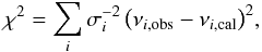 (17)where
νi,obs and
νi,cal are the observed and calculated
fluence frequencies in the i-bin respectively.
(17)where
νi,obs and
νi,cal are the observed and calculated
fluence frequencies in the i-bin respectively.
In the next step, the code re-starts the process with a new set of parameters, which are allowed to vary within established intervals. The procedure is stopped when a minimum of the χ2 test is found. In reality, the set of parameters that minimize the χ2 is not exactly the same for all energy bands. Assuming a Band spectrum with the same exponents α and β for all simulated events certainly contributes to these differences and, to remedy this situation, a higher weight was given to the parameters determined from the widest energy band, that is 15−150 keV.
The calculations were performed by using the facilities of the computation center (SIGAMM) of the Observatoire de la Côte d’Azur. On average, about five CPU.h are necessary to optimize a pair of parameters for the isotropic model, while about ten CPU.h are required for the jet-model, including or excluding evolution of the mean energy.
4. Results
To check our procedure, the code was tested without the beaming correction in order to compare our results with those in the literature obtained under the same condition. In this case, steps (3) and (4) of the code (see Sect. 2.1) were skipped since there is no need to verify the alignment of the jet with the observer’s direction.
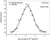 |
Fig. 1 Frequency distribution of fluences in the energy band 15−150 keV. Points correspond to data derived from the Swift-BAT catalog and the error bars indicate the bin width. The solid line corresponds to simulations assuming an isotropic emission model. The energy distribution defining the model is a log-normal distribution characterized by a median log Eiso = 50.96 (erg) and a dispersion σlog E = 0.92. |
Figure 1 shows the best fit of the observed frequency distribution of fluences by simulated data in the energy band 15−150 keV. Simulated fluences were computed with a log-normal energy Eiso distribution, whose median is log Eiso = 50.96 ± 0.34 and whose dispersion is σlog E = 0.92 ± 0.18. Errors indicate the uncertainties with respect to the fit of fluences in different energy bands. An early investigation by Jimenez et al. (2001), who have also assumed a log-normal distribution for the isotropic energy, led to a mean burst energy of log Eiso = 53.11 ± 0.20, about two orders of magnitude higher, but based on a sample of only eight objects. In Fig. 2 the observed frequency distribution of isotropic energies is shown in comparison with the true distribution derived from our simulations, characterized by the parameters just mentioned. The data corresponds to 170 events listed in the online Swift-BAT integrated parameters catalog (Butler et al. 2010). These data can be quite well fitted by a log-normal distribution with a median log Eiso = 52.73 and a dispersion σlog E = 0.88. These results indicate that in reality, even in the context of the isotropic emission model the mean energy released by GRB events is about 60 times lower than the value derived directly from observation. This difference is due to the well-known Malmquist bias, which favors the detection of the more energetic events and shifts the energy distribution toward higher values, as can be seen in Fig. 2. In fact, when these selection effects are taken into account, the isotropic energy of bursts increases with the redshift according to the analysis by Wu et al. (2012), suggesting an evolution of the energy distribution function.
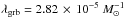
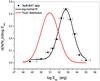 |
Fig. 2 Frequency distribution of isotropic energies. The red curve shows the true energy distribution derived from simulations. Points represent Swift-BAT data for 170 events and error bars indicate the bin width. The solid black curve is a log-normal fit of data. |
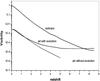 |
Fig. 3 Visibilities derived from our simulations as a function of redshift and for three different models: isotropic emission, jet without energy evolution, and jet including evolution characterized by a parameter δ = 0.5. Note that these visibilities correspond to the sensitivity of the Swift-BAT detector. |
One of the most important results derived from our simulations is the visibility function
v(z), which measures the fraction of bursts generated in
a given redshift interval that are effectively seen by the detector, in other words, events
in the line of sight able to trigger the detector. The visibility function is essentially
given by the ratio between bursts detected according to our rules in a given redshift
interval and the total number of bursts generated in the same redshift interval. As we
emphasized above, our detection criterion uses the average and not the peak flux. In this
case, the visibility function is probably slightly underestimated. In Fig. 3 the visibility function is shown for three different sets
of simulations: the isotropic model just discussed and jet models with and without energy
evolution to be analyzed below. As expected, the visibility for the jet model without
evolution is lower than that derived for the isotropic model, because not all events are
aligned with the observer. When a moderate energy evolution is included
(δ = 0.5), the resulting visibility is slightly lower than that of the jet
model without evolution up to z ~ 1.5 and then increases because the events
become more energetic, being able to trigger the detector. Beyond z ~ 7.5
this is true even if a comparison is made with the isotropic model (without evolution), as
can be seen in Fig. 3. If the visibility function
v(z) is known, the expected event rate can be computed
by the equation  (18)where
Kgrb = 4πλgrb(c/H0)3 = 9.89 × 10¹¹λgrb.
The numerical value is obtained if the fraction of mass of the formed stars originating in
GRB events (λgrb) is given in
(18)where
Kgrb = 4πλgrb(c/H0)3 = 9.89 × 10¹¹λgrb.
The numerical value is obtained if the fraction of mass of the formed stars originating in
GRB events (λgrb) is given in
 ,
the CSFR (R∗(z)) is given in
M⊙ Mpc-3 yr-1, and the event rate
dTgrb/dt is in
yr-1. Moreover, in the equation above, r(z)
is the comoving distance in units of the Hubble radius given by
,
the CSFR (R∗(z)) is given in
M⊙ Mpc-3 yr-1, and the event rate
dTgrb/dt is in
yr-1. Moreover, in the equation above, r(z)
is the comoving distance in units of the Hubble radius given by
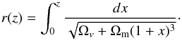 (19)For the considered energy
distribution, the numerical value of the integral in Eq. (18) is 4.71 × 10⁻³, implying a GRB rate of
dTgrb/dt = 4.66 × 10⁹λgrb
yr-1. Swift data indicate an all-sky frequency of 2.45
bursts/day (Gehrels et al. 2004) and, using the
observed fraction of long GRBs, the observed frequency of these events is 2.0 bursts/day.
Comparing this with our theoretical rate, this implies
(19)For the considered energy
distribution, the numerical value of the integral in Eq. (18) is 4.71 × 10⁻³, implying a GRB rate of
dTgrb/dt = 4.66 × 10⁹λgrb
yr-1. Swift data indicate an all-sky frequency of 2.45
bursts/day (Gehrels et al. 2004) and, using the
observed fraction of long GRBs, the observed frequency of these events is 2.0 bursts/day.
Comparing this with our theoretical rate, this implies
 .
This value should be compared with the value derived by Salvaterra & Chincarini (2007)
.
This value should be compared with the value derived by Salvaterra & Chincarini (2007) based on similar assumptions, that is isotropic emission and no evolution on the burst
energetics. Using our adopted local star formation rate of 0.0103
M⊙ Mpc-3 yr-1, one obtains a local
formation rate for LGRBs of Rgrb = 1.6
Gpc-3 yr-1. Despite the common assumptions (isotropy and no
evolution), Salvaterra & Chincarini (2007)
adopted a different procedure to compute the local formation rate: their analysis was based
on the burst luminosity function, while we considered the bolometric energy distribution.
Moreover, our burst detection criterion is quite different, which may explain the difference
of one order of magnitude between the two estimates of the local formation rate.
based on similar assumptions, that is isotropic emission and no evolution on the burst
energetics. Using our adopted local star formation rate of 0.0103
M⊙ Mpc-3 yr-1, one obtains a local
formation rate for LGRBs of Rgrb = 1.6
Gpc-3 yr-1. Despite the common assumptions (isotropy and no
evolution), Salvaterra & Chincarini (2007)
adopted a different procedure to compute the local formation rate: their analysis was based
on the burst luminosity function, while we considered the bolometric energy distribution.
Moreover, our burst detection criterion is quite different, which may explain the difference
of one order of magnitude between the two estimates of the local formation rate.
4.1. Jet models: local formation rates
Jet models were investigated under two main assumptions. In the first series of runs, the median of the jet energy distribution was kept constant, while in the second series of models the median was allowed to evolve with redshift according to Eq. (3). In this case, for a given value of the parameter δ, the code searches for the best fit of the observed fluence distribution by varying the median and the dispersion of the log-normal representing the true jet energy distribution, following the same procedure as described above. Figure 4 shows the best fit of the observed fluence frequency distribution by simulated data based on the jet model without evolution in the energy distribution. In this case, the model providing the best fit corresponds to a log-normal jet energy distribution with a median log EJ = 49.26 ± 0.18 and a dispersion σlog EJ = 0.43 ± 0.21. Note that the distribution energy of the jet model is narrower than that derived for the isotropic model. As expected, the jet model implies an average energy released in the form of γ-rays about 54 times lower than the isotropic model. The reduction factor is still higher (about 3200) when the comparison is made with the mean isotropic value deduced directly from observations, alleviating, as expected, the energy budget of these explosive events.
For a jet model without evolution the numerical integral in Eq. (18) is 2.35 × 10⁻⁵, leading
to  and a local GRB formation rate of 324 Gpc-3 yr-1, which is about
200 times higher than the rate derived under the assumption that the emission is
isotropic.
and a local GRB formation rate of 324 Gpc-3 yr-1, which is about
200 times higher than the rate derived under the assumption that the emission is
isotropic.
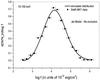 |
Fig. 4 Fluence frequency distribution for the jet model without energy evolution. Points correspond to Swift-BAT data as in Fig. 1. The solid curve was derived from simulations using a log-normal for the jet energy distribution defined by a median log EJ = 49.26 (erg) and a dispersion σlog E = 0.43. |
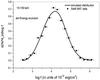 |
Fig. 5 Fluence frequency distribution for the jet model including energy evolution (δ = 0.5). Points correspond to Swift-BAT data as in Fig. 1. The solid curve was derived from simulations using a log-normal distribution for the jet energy distribution in which the median varies linearly with the redshift. |
When evolutionary effects are included in the energy distribution, the best fit of the
observed frequency distribution of fluences for δ = 0.5 was obtained with
a log-normal distribution defined by the parameters
log E0 = 48.46 ± 0.26 and
σlog EJ = 0.39 ± 0.24, as
shown in Fig. 5. In this particular model, the mean
jet energy at z = 1 is log EJ = 49.18, while
at z = 7 the mean value is log EJ = 50.48,
that is about 20 times higher. In Fig. 6 the
frequency distribution of jet energies corresponding to the detected events is shown. Note
that the distribution is not symmetric, but has an extended high-energy wing because of
the evolution of the energy distribution. From this distribution the mean expected value
of the jet energy is log EJ = 49.48. It is worth mentioning
that this value derived from simulations compares quite well with the mean jet energy
resulting from the sample of GRBs with prominent jet breaks by Racusin et al. (2009), that is
log EJ = 49.64 and with the mean jet energy derived by Schmidt (2001), that is
log EJ = 49.69. The numerical integral in Eq. (18) is in this particular case equal to
2.62 × 10⁻⁵, resulting in a formation fraction of GRBs of
 and in a local formation rate of 290 Gpc-3 yr-3. Thus, the
introduction of a moderate evolution in the jet energy distribution does not significantly
change the estimate of the local formation rate. It is interesting that Lu at al. (2012)
also found a similar local formation rate (Rgrb = 285
Gpc-3 yr-1), but their analysis is based on a possible
anti-correlation between the opening angle and the redshift.
and in a local formation rate of 290 Gpc-3 yr-3. Thus, the
introduction of a moderate evolution in the jet energy distribution does not significantly
change the estimate of the local formation rate. It is interesting that Lu at al. (2012)
also found a similar local formation rate (Rgrb = 285
Gpc-3 yr-1), but their analysis is based on a possible
anti-correlation between the opening angle and the redshift.
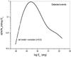 |
Fig. 6 Frequency distribution of energies for the jet model including evolution (δ = 0.5). The distribution corresponds to detected events only. |
4.2. Redshift distribution
Previous investigations on the redshift distribution of GRBs led to the conclusion that without evolution either in the luminosity function or/and in the formation efficiency of GRBs, the number of events at high redshift is underestimated if the formation rate simply follows the CSFR. Since then, the number of GRBs with measured redshift has increased considerably, permitting more robust analyses. To compare the present data with our simulations, the redshift frequency distribution was calculated using 189 events given in the online Swift-BAT catalog of integrated parameters (Butler 2010).
Considering the difficulty to model the selection effects that affect the detection of
the GRB host galaxy and the redshift measurement, they are not considered here. In this
case, defining
Ngrb = dTgrb/dt,
the expected redshift distribution resulting from our simulations is 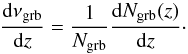 (20)In Fig. 7 we show the simulated redshift distributions for the
three cases considered in the present investigation and data for 189 events. As expected,
the isotropic and the jet models without evolution underestimate the frequency of events
for z > 2. Including a moderate evolution in the
jet energy distribution permits a better representation of data, in agreement with
previous investigations. Note that this evolutionary jet model predicts a fraction of
events for z ≥ 6 equal to 0.022, which corresponds to four events for a
sample of 189 objects, in good agreement with the fact that four events with
z ≥ 6 are present in the considered sample.
(20)In Fig. 7 we show the simulated redshift distributions for the
three cases considered in the present investigation and data for 189 events. As expected,
the isotropic and the jet models without evolution underestimate the frequency of events
for z > 2. Including a moderate evolution in the
jet energy distribution permits a better representation of data, in agreement with
previous investigations. Note that this evolutionary jet model predicts a fraction of
events for z ≥ 6 equal to 0.022, which corresponds to four events for a
sample of 189 objects, in good agreement with the fact that four events with
z ≥ 6 are present in the considered sample.
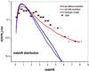 |
Fig. 7 Frequency distribution of LGRB redshifts. Data are from online Swift-BAT integrated parameter and error bars indicate the bin width. The different curves correspond to distributions derived from the present simulations: isotropic (blue curve) and jet (black curve) models without evolution and jet model including evolution (red curve). |
4.3. Supernova connection
Observations seem to suggest that at least a fraction of LGRBs are linked to type Ibc supernova, whose spectra are dominated by broad absorption lines. Most of the associated bursts have isotropic energies of about 1049 erg and are assumed to have jets with wide opening angles (EJ ~ Eiso). It is not clear yet if these low luminosity bursts (LL GRBs) constitute a particular subclass of the LGRBs (Liang et al. 2007; Guetta & Della Valle 2007). According to estimates by Soderberg et al. (2006a), the rate of LL GRBs is about 230 Gpc-3 yr-1, similar to the rate currently derived for LGRBs. However, Guetta & Della Valle (2007) concluded that energetic LGRBs represent only a small fraction of LL GRBs. This clearly is an open question.
The fraction by mass λgrb of formed stars giving origin to
LGRBs was estimated in the present study to be  .
If the initial mass function (IMF) ζ(m) is known,
λgrb fixes the lower mass limit
mgrb of progenitors of LGRBs by the relation
.
If the initial mass function (IMF) ζ(m) is known,
λgrb fixes the lower mass limit
mgrb of progenitors of LGRBs by the relation  (21)Using the IMF by
Miller & Scalo (1979) normalized in the
mass interval 0.1−125 M⊙, from the equation above, one
obtains that the progenitors of LGRBs must have a minimum mass of about 90
M⊙. On the other hand, Georgy et al. (2009) estimated based on rotating stellar models computed by
Meynet & Maeder (2003, 2005) that for solar metallicities the minimum mass of
the progenitors of type Ic supernovae is about 39 M⊙. Thus,
from Eq. (21) one obtains
(21)Using the IMF by
Miller & Scalo (1979) normalized in the
mass interval 0.1−125 M⊙, from the equation above, one
obtains that the progenitors of LGRBs must have a minimum mass of about 90
M⊙. On the other hand, Georgy et al. (2009) estimated based on rotating stellar models computed by
Meynet & Maeder (2003, 2005) that for solar metallicities the minimum mass of
the progenitors of type Ic supernovae is about 39 M⊙. Thus,
from Eq. (21) one obtains
 for the fraction by mass of formed stars that become type Ic supernovae. These values
imply that only ~9.0% of SNIc could be associated with LGRBs, namely, only those with a
very massive progenitor. Instead of using lower mass limits derived theoretically, it is
possible to directly compare the present derived formation rate of LGRBs with the SNIbc
rate estimated from observations. Using data by Cappellaro
et al. (1999) for rates of core-collapsed supernovae and the ratio between
different supernova types derived by Prieto et al.
(2008), we estimated that
RSNIbc ~ 2.7 × 10⁴
Gpc-3 yr-1. Comparing this with the LGRB rate derived in this
work, one concludes that only ~1% of type Ic supernovae could be related with LGRBs. Note
that the SNIbc rate estimated from observations implies progenitor masses lower than those
derived theoretically, that is around 16 M⊙. However, these
results indicate that the majority of SNIbc are not related to LGRBs, in agreement with
the conclusions by Soderberg et al. (2006b).
However, it is worth mentioning that recent radio observations of two SNIbc supernovae
(Soderberg et al. 2010) and 2007gr (Paragi et al. 2010) not associated with a
γ-flash indicate the presence of mildly relativistic outflows, which
require a central engine able to power the observed flows.
for the fraction by mass of formed stars that become type Ic supernovae. These values
imply that only ~9.0% of SNIc could be associated with LGRBs, namely, only those with a
very massive progenitor. Instead of using lower mass limits derived theoretically, it is
possible to directly compare the present derived formation rate of LGRBs with the SNIbc
rate estimated from observations. Using data by Cappellaro
et al. (1999) for rates of core-collapsed supernovae and the ratio between
different supernova types derived by Prieto et al.
(2008), we estimated that
RSNIbc ~ 2.7 × 10⁴
Gpc-3 yr-1. Comparing this with the LGRB rate derived in this
work, one concludes that only ~1% of type Ic supernovae could be related with LGRBs. Note
that the SNIbc rate estimated from observations implies progenitor masses lower than those
derived theoretically, that is around 16 M⊙. However, these
results indicate that the majority of SNIbc are not related to LGRBs, in agreement with
the conclusions by Soderberg et al. (2006b).
However, it is worth mentioning that recent radio observations of two SNIbc supernovae
(Soderberg et al. 2010) and 2007gr (Paragi et al. 2010) not associated with a
γ-flash indicate the presence of mildly relativistic outflows, which
require a central engine able to power the observed flows.
We emphasize that if the progenitors of LGRBs are not single stars, our analysis is invalid. This is also true if the IMF evolves as assumed by Wang & Dai (2011), who proposed an IMF that becomes increasingly top-heavy at high reshift, producing higher LGRB rates at high z.
5. Conclusions
We reported results based on Monte Carlo simulations aimed at studying the properties of LGRBs. Mock catalogs of LGRBs derived from these simulations permitted us to predict observed fluences, and from the comparison with actual data, we were able to estimate the parameters that define the energy distribution of LGRBs. These simulations permitted us also to compute the visibility function that measures the probability for a given burst generated at a given redshift z to be able to trigger the Swift-BAT detector.
When an isotropic emission model without evolution is considered, the observed fluence distribution derived from the Swift-BAT catalog can be reproduced by an energy distribution modeled by a log-normal characterized by a median log Eiso = 50.95 (erg) and a dispersion σlog E = 0.92. When a comparison is made with the mean energy derived directly from observations, we realize that due to the Malmquist bias, the aforementioned intrinsic (simulated) value is about 60 times lower. The local formation rate of LGRBs derived from our simulations under the assumption of isotropic emission is Rgrb = 1.6 Gpc-3 yr-1, an intermediate value when compared with those derived by Salvaterra & Chincarini (2007) and Pélangeon et al. (2008). The present local formation rate based on the isotropic emission model agrees with the result by Wanderman & Piran (2010), but we emphasize that in their approach evolution effects are present in the luminosity function of GRBs. The formation rate of subluminous LGRBs (under the assumption of isotropic emission) could be considerably higher. Howell & Coward (2013) derived a formation rate of ~150 Gpc-3 yr-1 for these events.
For beamed emission model without evolution of the energy distribution is considered, the observed fluence distribution can be fitted by simulated data when a log-normal defined by a median log EJ = 49.26 (in erg) and a dispersion σlog E = 0.43 represent the intrinsic energy distribution of LGRBs. As expected, these results considerably alleviate the energy requirements for GRBs models. The resulting local formation rate for this model is Rrgb = 324 Gpc-3 yr-1. Frail et al. (2001) obtained a local formation rate in the context of the jet model of Rgrb ~ 250 Gpc-3 yr-1, similar to our result this agreement is fortuitous for the following reason: they took the isotropic rate given by Schmidt (2001) and corrected this value by the harmonic mean of the beaming fraction. A similar reasoning was given by Lamb et al. (2005) in their estimates of the local formation rate.
The redshift distribution predicted by the isotropic and the jet models without evolutionary effects underestimates the number of LGRBs occurring at z > 2, in agreement with previous investigations concluding the necessity of a moderate/strong evolution of the luminosity function. The model prediction of the observed redshift distribution (currently including 189 objects) can be considerably improved if the jet energy distribution evolves in the sense that at high redshift bursts are more energetic. Such an evolution was modeled in our simulations by assuming that the median of the log-normal describing the energy distribution varies as Emed,J ∝ eδ(1 + z). Different set of simulations were performed by varying the slope dlgEmed/d(1 + z) = δ, and the best representation was found for δ = 0.5 (see Fig. 7). The ratio between the mean jet energies for events produced at z = 7 and z = 1 is about 20, indicating a moderate evolution in the energy distribution. For this model, the derived local formation is Rgrb = 290 Gpc-3 yr-1 and the expected average jet energy is 3.0 × 1049 erg, in agreement with the value derived by Lu et al. (2012). Nevertheless, these authors have considered the opening angle to be related to the redshift, while in our simulations both quantities were statistically independent.
The aforementioned evolutionary jet model led to a fraction by mass of formed stars
originating in LGRBs of .
If the IMF does not evolve and a Miller & Scalo
(1979) IMF is adopted, the derived value of λgrb
implies that the minimum mass to produce an LGRB is 90 M⊙,
indicating that only very massive stars are associated to these events. Moreover, the ratio
between LGRBs and the SNIbc formation rates is in the range 0.01−0.09, supporting the idea
that stars less massive than the above limit may produce an SNIbc event, but not necessarily
an LGRB.
Acknowledgments
C.K. acknowledges the financial support from the University of Nice-Sophia Antipolis for her Ph.D. project. The authors also thank J.-L. Atteia and T. Regimbau for the critical reading of the manuscript.
References
- Amati, L., Guidorzi, C., Frontera, F., et al. 2008, MNRAS, 391, 577 [NASA ADS] [CrossRef] [MathSciNet] [Google Scholar]
- Amati, L., Frontera, F., & Guidorzi, C. 2009, A&A, 508, 173 [NASA ADS] [CrossRef] [EDP Sciences] [Google Scholar]
- Band, D. L. 2006, ApJ, 644, 378 [NASA ADS] [CrossRef] [Google Scholar]
- Band, D., Matteson, J., Ford, L., et al. 1993, ApJ, 413, 281 [NASA ADS] [CrossRef] [Google Scholar]
- Berger, E. 2011, New Astron. Rev., 55, 1 [NASA ADS] [CrossRef] [Google Scholar]
- Berger, E., Chornock, R., Holmes, T. R., et al. 2011, ApJ, 743, 204 [NASA ADS] [CrossRef] [Google Scholar]
- Butler, N. 2010, SWIFT BAT Integrated Spectral Parameters, http://butler.lab.asu.edu/swift/bat_spec_table.html [Google Scholar]
- Butler, N. R., Bloom, J. S., & Poznanski, D. 2010, ApJ, 711, 495 [NASA ADS] [CrossRef] [Google Scholar]
- Cao, X.-F., Yu, Y.-W., Cheng, K. S., & Zheng, X.-P. 2011, MNRAS, 416, 2174 [NASA ADS] [CrossRef] [Google Scholar]
- Cappellaro, E., Evans, R., & Turatto, M. 1999, A&A, 351, 459 [NASA ADS] [Google Scholar]
- Church, R. P., Levan, A. J., Davies, M. B., & Tanvir, N. 2011, MNRAS, 413, 2004 [NASA ADS] [CrossRef] [Google Scholar]
- Cole, S., Norberg, P., Baugh, C. M., et al. 2001, MNRAS, 326, 255 [NASA ADS] [CrossRef] [Google Scholar]
- Coward, D. M. 2005, MNRAS, 360, L77 [NASA ADS] [CrossRef] [Google Scholar]
- Dai, Z. G., & Cheng, K. S. 2001, ApJ, 558, L109 [NASA ADS] [CrossRef] [Google Scholar]
- Daigne, F., Rossi, E. M., & Mochkovitch, R. 2006, MNRAS, 372, 1034 [NASA ADS] [CrossRef] [Google Scholar]
- de Araujo, F. X., & de Freitas Pacheco, J. A. 1994, Ap&SS, 219, 267 [NASA ADS] [CrossRef] [Google Scholar]
- de Araujo, F. K., de Freitas-Pacheco, J. A., & Petrini, D. 1994, MNRAS, 267, 501 [NASA ADS] [CrossRef] [Google Scholar]
- Filloux, C., Durier, F., Pacheco, J. A. F., & Silk, J. 2010, Int. J. Mod. Phys. D, 19, 1233 [NASA ADS] [CrossRef] [Google Scholar]
- Filloux, C., de Freitas Pacheco, J. A., Durier, F., & de Araujo, J. C. N. 2011, Int. J. Mod. Phys. D, 20, 2399 [NASA ADS] [CrossRef] [Google Scholar]
- Frail, D. A., Kulkarni, S. R., Sari, R., et al. 2001, ApJ, 562, L55 [NASA ADS] [CrossRef] [Google Scholar]
- Fruchter, A. S., Levan, A. J., Strolger, L., et al. 2006, Nature, 441, 463 [NASA ADS] [CrossRef] [PubMed] [Google Scholar]
- Gehrels, N., Chincarini, G., Giommi, P., et al. 2004, ApJ, 611, 1005 [NASA ADS] [CrossRef] [Google Scholar]
- Georgy, C., Meynet, G., Walder, R., Folini, D., & Maeder, A. 2009, A&A, 502, 611 [NASA ADS] [CrossRef] [EDP Sciences] [Google Scholar]
- Ghirlanda, G., Ghisellini, G., & Lazzati, D. 2004, ApJ, 616, 331 [NASA ADS] [CrossRef] [Google Scholar]
- Goldstein, A., Preece, R. D., Briggs, M. S., et al. 2011, ApJ, submitted [arXiv:1101.2458] [Google Scholar]
- Guetta, D., & Della Valle, M. 2007, ApJ, 657, L73 [NASA ADS] [CrossRef] [Google Scholar]
- Hjorth, J., Sollerman, J., Møller, P., et al. 2003, Nature, 423, 847 [NASA ADS] [CrossRef] [PubMed] [Google Scholar]
- Hopkins, A. M., & Beacom, J. F. 2006, ApJ, 651, 142 [NASA ADS] [CrossRef] [MathSciNet] [Google Scholar]
- Horváth, I., Balázs, L. G., Bagoly, Z., & Veres, P. 2008, A&A, 489, L1 [NASA ADS] [CrossRef] [EDP Sciences] [Google Scholar]
- Horváth, I., Bagoly, Z., Balázs, L. G., et al. 2010, ApJ, 713, 552 [NASA ADS] [CrossRef] [Google Scholar]
- Howell, E. J., & Coward, D. M. 2013, MNRAS, 428, 167 [NASA ADS] [CrossRef] [Google Scholar]
- Huja, D., Mészáros, A., & Řípa, J. 2009, A&A, 504, 67 [NASA ADS] [CrossRef] [EDP Sciences] [Google Scholar]
- Imerito, A., Coward, D., Burman, R., & Blair, D. 2008, MNRAS, 391, 405 [NASA ADS] [CrossRef] [Google Scholar]
- Jimenez, R., Band, D., & Piran, T. 2001, ApJ, 561, 171 [NASA ADS] [CrossRef] [Google Scholar]
- Kouveliotou, C., Meegan, C. A., Fishman, G. J., et al. 1993, ApJ, 413, L101 [NASA ADS] [CrossRef] [Google Scholar]
- Lamb, D. Q., Donaghy, T. Q., & Graziani, C. 2005, ApJ, 620, 355 [NASA ADS] [CrossRef] [Google Scholar]
- Liang, E., Zhang, B., Virgili, F., & Dai, Z. G. 2007, ApJ, 662, 1111 [NASA ADS] [CrossRef] [Google Scholar]
- Lu, R.-J., Wei, J.-J., Qin, S.-F., & Liang, E.-W. 2012, ApJ, 745, 168 [NASA ADS] [CrossRef] [Google Scholar]
- Meszaros, P., Rees, M. J., & Wijers, R. A. M. J. 1999, New A, 4, 303 [NASA ADS] [CrossRef] [Google Scholar]
- Meynet, G., & Maeder, A. 2003, A&A, 404, 975 [NASA ADS] [CrossRef] [EDP Sciences] [Google Scholar]
- Meynet, G., & Maeder, A. 2005, A&A, 429, 581 [Google Scholar]
- Miller, G. E., & Scalo, J. M. 1979, ApJS, 41, 513 [NASA ADS] [CrossRef] [Google Scholar]
- Murase, K., Ioka, K., Nagataki, S., & Nakamura, T. 2006, ApJ, 651, L5 [NASA ADS] [CrossRef] [Google Scholar]
- Paragi, Z., Taylor, G. B., Kouveliotou, C., et al. 2010, Nature, 463, 516 [NASA ADS] [CrossRef] [PubMed] [Google Scholar]
- Pélangeon, A., Atteia, J.-L., Nakagawa, Y. E., et al. 2008, A&A, 491, 157 [NASA ADS] [CrossRef] [EDP Sciences] [Google Scholar]
- Prantzos, N., & Boissier, S. 2003, A&A, 406, 259 [NASA ADS] [CrossRef] [EDP Sciences] [Google Scholar]
- Prieto, J. L., Stanek, K. Z., & Beacom, J. F. 2008, ApJ, 673, 999 [NASA ADS] [CrossRef] [Google Scholar]
- Qin, S.-F., Liang, E.-W., Lu, R.-J., Wei, J.-Y., & Zhang, S.-N. 2010, MNRAS, 406, 558 [NASA ADS] [CrossRef] [Google Scholar]
- Racusin, J. L., Liang, E. W., Burrows, D. N., et al. 2009, ApJ, 698, 43 [NASA ADS] [CrossRef] [Google Scholar]
- Rhoads, J. E. 1997, ApJ, 487, L1 [NASA ADS] [CrossRef] [Google Scholar]
- Rhoads, J. E. 1999, ApJ, 525, 737 [NASA ADS] [CrossRef] [Google Scholar]
- Rossi, E., Lazzati, D., & Rees, M. J. 2002, MNRAS, 332, 945 [NASA ADS] [CrossRef] [Google Scholar]
- Sakamoto, T., Barthelmy, S. D., Baumgartner, W. H., et al. 2011, ApJS, 195, 2 [NASA ADS] [CrossRef] [Google Scholar]
- Salvaterra, R., & Chincarini, G. 2007, ApJ, 656, L49 [NASA ADS] [CrossRef] [Google Scholar]
- Schmidt, M. 2001, ApJ, 552, 36 [NASA ADS] [CrossRef] [Google Scholar]
- Soderberg, A. M., Kulkarni, S. R., Nakar, E., et al. 2006a, Nature, 442, 1014 [CrossRef] [Google Scholar]
- Soderberg, A. M., Nakar, E., Berger, E., & Kulkarni, S. R. 2006b, ApJ, 638, 930 [NASA ADS] [CrossRef] [PubMed] [Google Scholar]
- Soderberg, A. M., Chakraborti, S., Pignata, G., et al. 2010, Nature, 463, 513 [NASA ADS] [CrossRef] [Google Scholar]
- Stanek, K. Z., Matheson, T., Garnavich, P. M., et al. 2003, ApJ, 591, L17 [NASA ADS] [CrossRef] [Google Scholar]
- Virgili, F. J., Zhang, B., Nagamine, K., & Choi, J.-H. 2011, MNRAS, 417, 3025 [NASA ADS] [CrossRef] [Google Scholar]
- Wanderman, D., & Piran, T. 2010, MNRAS, 406, 1944 [NASA ADS] [Google Scholar]
- Wang, F. Y., & Dai, Z. G. 2011, ApJ, 727, L34 [NASA ADS] [CrossRef] [Google Scholar]
- Woosley, S. E., & Bloom, J. S. 2006, ARA&A, 44, 507 [NASA ADS] [CrossRef] [Google Scholar]
- Wu, S.-W., Xu, D., Zhang, F.-W., & Wei, D.-M. 2012, MNRAS, 423, 2627 [NASA ADS] [CrossRef] [Google Scholar]
All Figures
|
Fig. 1 Frequency distribution of fluences in the energy band 15−150 keV. Points correspond to data derived from the Swift-BAT catalog and the error bars indicate the bin width. The solid line corresponds to simulations assuming an isotropic emission model. The energy distribution defining the model is a log-normal distribution characterized by a median log Eiso = 50.96 (erg) and a dispersion σlog E = 0.92. |
| In the text | |
|
Fig. 2 Frequency distribution of isotropic energies. The red curve shows the true energy distribution derived from simulations. Points represent Swift-BAT data for 170 events and error bars indicate the bin width. The solid black curve is a log-normal fit of data. |
| In the text | |
|
Fig. 3 Visibilities derived from our simulations as a function of redshift and for three different models: isotropic emission, jet without energy evolution, and jet including evolution characterized by a parameter δ = 0.5. Note that these visibilities correspond to the sensitivity of the Swift-BAT detector. |
| In the text | |
|
Fig. 4 Fluence frequency distribution for the jet model without energy evolution. Points correspond to Swift-BAT data as in Fig. 1. The solid curve was derived from simulations using a log-normal for the jet energy distribution defined by a median log EJ = 49.26 (erg) and a dispersion σlog E = 0.43. |
| In the text | |
|
Fig. 5 Fluence frequency distribution for the jet model including energy evolution (δ = 0.5). Points correspond to Swift-BAT data as in Fig. 1. The solid curve was derived from simulations using a log-normal distribution for the jet energy distribution in which the median varies linearly with the redshift. |
| In the text | |
|
Fig. 6 Frequency distribution of energies for the jet model including evolution (δ = 0.5). The distribution corresponds to detected events only. |
| In the text | |
|
Fig. 7 Frequency distribution of LGRB redshifts. Data are from online Swift-BAT integrated parameter and error bars indicate the bin width. The different curves correspond to distributions derived from the present simulations: isotropic (blue curve) and jet (black curve) models without evolution and jet model including evolution (red curve). |
| In the text | |
Current usage metrics show cumulative count of Article Views (full-text article views including HTML views, PDF and ePub downloads, according to the available data) and Abstracts Views on Vision4Press platform.
Data correspond to usage on the plateform after 2015. The current usage metrics is available 48-96 hours after online publication and is updated daily on week days.
Initial download of the metrics may take a while.