| Issue |
A&A
Volume 559, November 2013
|
|
|---|---|---|
| Article Number | A23 | |
| Number of page(s) | 14 | |
| Section | Interstellar and circumstellar matter | |
| DOI | https://doi.org/10.1051/0004-6361/201220581 | |
| Published online | 30 October 2013 | |
Turbulent entrainment origin of protostellar outflows
1
Max-Planck Institut für Radioastronomie,
Auf dem Hügel, 69,
53121
Bonn,
Germany
e-mail:
This email address is being protected from spambots. You need JavaScript enabled to view it.
2
School of Astronomy and Space Science, Nanjing
University, Nanjing
210093, PR
China
Received:
17
October
2012
Accepted:
27
August
2013
Abstract
Protostellar outflow is a prominent process that accompanies the formation of stars. It is generally agreed that wide-angled protostellar outflows come from the interaction between the wind from a forming star and the ambient gas. However, it is still unclear how the interaction takes place. In this work, we theoretically investigate the possibility that the outflow results from interaction between the wind and the ambient gas in the form of turbulent entrainment. In contrast to the previous models, turbulent motion of the ambient gas around the protostar is taken into account. In our model, the ram-pressure of the wind balances the turbulent ram-pressure of the ambient gas, and the outflow consists of the ambient gas entrained by the wind. The calculated outflow from our modelling exhibits a conical shape. The total mass of the outflow is determined by the turbulent velocity of the envelope as well as the outflow age, and the velocity of the outflow is several times higher than the velocity dispersion of the ambient gas. The outflow opening angle increases with the strength of the wind and decreases with the increasing ambient gas turbulence. The outflow exhibits a broad line width at every position. We propose that the turbulent entrainment process, which happens ubiquitously in nature, plays a universal role in shaping protostellar outflows.
Key words: stars: winds, outflows / stars: massive / ISM: jets and outflows / ISM: kinematics and dynamics / turbulence / line: profiles
© ESO, 2013
1. Introduction
Protostellar outflow is a prominent process that is intimately connected with the formation of stars. When a protostar accretes gas from its surroundings, it produces a powerful wind or jet. As the wind or jet material moves away from the protostar, ambient gas is entrained. The mixture of the wind or jet gas and the ambient gas will move away from the protostar, forming a so-called molecular outflow. In observations of the star-forming regions with rotational transitions of molecules such as CO, outflows can be easily identified from the high-velocity part of the emission line. The physical size of the molecular outflow is about a parsec. The typical velocity of the outflowing gas is about tens of kilometers per second, and the morphology of the outflow can be collimated (jet-like) or less collimated (conical-shaped), or a combination of both.
Many of the outflows exhibit as conical-shaped geometry (Shepherd et al. 1998; Lee et al. 2000; Arce & Sargent 2006; Qiu et al. 2009; Ren et al. 2011; Cyganowski et al. 2011). It is still unclear how these conical-shaped outflows form. Models that can explain conical-shaped outflows include the wind-driven shell model (Shu et al. 1991; Li & Shu 1996; Lee et al. 2001) and the circulation model (Fiege & Henriksen 1996; Lery et al. 1999). In the wind-driven shell model, the wind from the protostar blows into the ambient medium, and a shell forms at the interface between the wind and the ambient gas. The shell absorbs momentum from the wind and expands. The outflowing material consists of the ambient gas swept up by the shell. In the circulation model, the gas circulates around the protostar in a quadrupolar way, and it is the gas that moves outward in this circulation cycle that constitutes the outflow.
Neither of these models properly addresses the role of supersonic turbulent motion in the
formation and evolution of the protostellar outflows. This might be because the importance
of supersonic turbulent motion in star-forming regions was not generally recognized when
these models were proposed. Today, it is widely recognized that the interstellar medium
where stars form is turbulent, this turbulence is supersonic in most star-forming regions
(Larson 1981; Ballesteros-Paredes et al. 2007). This will bring about serious physical
discrepancies to both models. For the wind-driven shell model, the turbulent ram-pressure
(expressed as  ) is much higher than
the thermal pressure, and is often comparable to the ram-pressure of the wind (expressed as
) is much higher than
the thermal pressure, and is often comparable to the ram-pressure of the wind (expressed as
 , see Sect. 4). Therefore the wind-driven shell model is no longer
valid since the physical condition cannot allow the shell to expand for long. The
circulation model is also questionable when the interstellar medium is turbulent, because
turbulent motion is expected to significantly distort the motion of gas, making the initial
condition unfavourable for circulation to occur.
, see Sect. 4). Therefore the wind-driven shell model is no longer
valid since the physical condition cannot allow the shell to expand for long. The
circulation model is also questionable when the interstellar medium is turbulent, because
turbulent motion is expected to significantly distort the motion of gas, making the initial
condition unfavourable for circulation to occur.
The kinematic structures of the outflows are only poorly reproduced by the previous models. Mappings of outflows with molecular lines reveal the spatial and velocity structures of the outflowing gas, which is crucial to test the models. It is found that the outflows ubiquitously exhibit a broad line width at different positions. Seen from position-velocity diagrams, the outflowing gas exhibits a wide velocity spread at one given position (Sect. 3). This is difficult to understand in the context of the widely accepted wind-driven shell model (Shu et al. 1991; Li & Shu 1996; Lee et al. 2001), because the shell swept by the wind will expand according to the Hubble law, and the expansion speed of the shell is higher in the directions where the shell has progressed further. Seen from the position-velocity diagram, we can identify two velocity components at one given position. One component comes from the front wall of the outflow cavity, the other from the back wall of the outflow cavity (Lee et al. 2000). However, observations found that at one single position, there is only one broad component (e.g. Qiu et al. 2009).
It is observationally found that the opening angles of outflows evolve significantly during their lifetimes (Beuther & Shepherd 2005; Arce & Sargent 2006). While usually interpreted as the evolution of the wind-envelope interaction (Arce & Sargent 2006), a comprehensive treatment of this interaction in the presence of the turbulent motion of the ambient gas is still lacking.
In this study, we theoretically investigate the formation of outflows from the turbulent mixing between the wind from the protostar and the turbulent ambient gas. In our wind-driven turbulent entrainment model, the ram-pressure of the wind and the turbulent ram-pressure of the ambient gas (envelope) establish hydrostatic balance, and the outflow is the gas contained in the turbulent entrainment layer between the wind and the turbulent envelope. In Sect. 2 we present the basic physical picture, followed by a detailed description of our model. In Sect. 3 we compare the image and position-velocity diagram from our model with existing observations. In Sects. 4.1 and 4.2 we offer a unified framework to understand outflows from low-mass protostars and high-mass protostars as well as AGN-driven outflows. We also discuss the possibility that the wind is not strong enough to push the envelope, and predict the existence of dwarf outflows in these situations (Sect. 4.3). In Sect. 5 we conclude.
Recently, the interaction between a wind and a turbulent core has been studied with radiation-hydrodynamic simulations (Offner et al. 2011), focusing on how the physical structure suggested by the simulations can be reproduced through millimetre-wavelength aperture synthesis observations. In this work, we present an explicit treatment of the mixing entrainment process, and study the consequences of this turbulent entrainment in producing protostellar outflows.
2. Model
In our model, the outflowing gas is contained in the turbulent entrainment layer that develops between the wind and the envelope (Fig. 1). The wind is collimated, and its strength reaches a maximum around the z-axis of Fig. 1. The wind is launched in a region close to the protostar due to magnetic centrifugal forces. This wind is generally collimated and exhibits universal asymptotic collimation properties (Shu et al. 1995; Matzner & McKee 1999). The wind evacuates a cavity and is confined mainly inside it. The ambient matter (envelope) is still present in regions father away from the outflow axis. The outflow layer lies between the cavity and the ambient matter. The outflow is generated by the interaction between the wind and the envelope.
The turbulent nature of the interstellar medium has been recognized for years. It has been suggested that it plays an important role in regulating the star formation processes inside molecular clouds (Plume et al. 1997; Krumholz & McKee 2005; Ballesteros-Paredes et al. 2007). Molecular outflows have been suggested as major drivers of this turbulent motion (Matzner 2007; Nakamura & Li 2007). The role of turbulence in the formation and evolution of the molecular outflow remains unexplored. It is easy to show (Sect. 4.1) that at physical scales of about a parsec (which is the typical physical scale of the outflow), turbulence dominates the dynamical properties of the medium. It is therefore necessary to consider the roles of turbulence consistently.
In this study, we propose that the structure of the outflow is determined by the following
processes: first, we propose that the wind and the envelope will establish hydrostatic
balance, and this balance will determine the shape of the outflow. According to Fig. 1, the wind has a ram-pressure that points away from the
protostar (see pwind in Fig. 1,
where  ), and the
envelope has a ram-pressure that is perpendicular to the wall of the outflow cavity
(penvelope). According to the balance of these two forces, the
shape of the outflow cavity can be numerically calculated (Sect. 2.2).
), and the
envelope has a ram-pressure that is perpendicular to the wall of the outflow cavity
(penvelope). According to the balance of these two forces, the
shape of the outflow cavity can be numerically calculated (Sect. 2.2).
 |
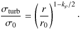
Fig. 1 Cartoon showing the basic structure of our model. The outflow (red region) lies between the wind and the envelope. Arrows (pwind and penvelope) denote the ram-pressure of the wind and the envelope. With wind we denote the cavity evacuated by the wind, with turbulent envelope we denote the turbulent envelope, and with outflow layer we denote the layer which contains the mixture of gas from the wind and gas from the envelope. |
Second, we propose that a turbulent mixing layer develops between the wind and the envelope. When the wind moves relative to the envelope, Kelvin-Helmholtz instability occurs. When the instability saturates, a mixing layer establishes. This mixing layer grows as it absorbs mass and momentum from the envelope and the wind. The mass and momentum of the mixing layer is determined by mass and momentum conservations (Sects. 2.3, 2.4).
Turbulence plays an important role in both processes. First, turbulence influences the turbulent ram-pressure of the envelope, and in turn influences the pressure balance between the wind and the envelope. Therefore, turbulence influences the shape of the outflow (Sect. 2.2 ). Second, turbulence changes the mixing process that occurs between the wind and the envelope. Therefore, it influences the mass and velocity of the outflow (Sects. 2.3, 2.4).
The structure of the molecular cloud is inhomogeneous at a variety of scales. On a parsec scale, millimeter/sub-millimeter studies suggest that the density distribution of molecular gas around the protostar is consistent with being spherically symmetric and can be described as a power-law ρ ~ rγ (e.g. Keto & Zhang 2010; Longmore et al. 2011).
Following these author we parametrized the density distribution of the envelope as
 (1)By assuming
hydrostatic equilibrium, Eq. (1) leads to the
distribution of the turbulent velocity σturb that takes the form
(McLaughlin & Pudritz 1996; McKee & Holliman 1999; McKee & Tan 2003)
(1)By assuming
hydrostatic equilibrium, Eq. (1) leads to the
distribution of the turbulent velocity σturb that takes the form
(McLaughlin & Pudritz 1996; McKee & Holliman 1999; McKee & Tan 2003)
 (2)The power-law index
kρ in Eq. (1) is set according to the observational studies by Beuther et al. (2002), Mueller et al.
(2002), Keto & Zhang (2010), Longmore et al. (2011). In our canonical model,
consulting the results in Longmore et al. (2011) we
set a density of 3.35 × 10⁻¹⁹ g cm-3 at r = 0.3pc
for Eq. (1). The parameter values are
summarized in Table 1. These parameters are set to be
typical of high-mass protostars (e.g. Keto & Zhang
2010; Longmore et al. 2011). Furthermore,
since our model is scale-free, the results can be scaled to different situations (Sect.
4.4).
(2)The power-law index
kρ in Eq. (1) is set according to the observational studies by Beuther et al. (2002), Mueller et al.
(2002), Keto & Zhang (2010), Longmore et al. (2011). In our canonical model,
consulting the results in Longmore et al. (2011) we
set a density of 3.35 × 10⁻¹⁹ g cm-3 at r = 0.3pc
for Eq. (1). The parameter values are
summarized in Table 1. These parameters are set to be
typical of high-mass protostars (e.g. Keto & Zhang
2010; Longmore et al. 2011). Furthermore,
since our model is scale-free, the results can be scaled to different situations (Sect.
4.4).
Summary of model parameters.
2.1. Wind from the embedded protostar
In our model, the outflow consists of the envelope gas entrained by the wind. To specify
the wind, we followed the formalism used by Lee et al.
(2001). In a spherical coordinate system (r,θ,φ), Shu et al. (1995) have shown that the radial velocity
of an X-wind is roughly constant, and the density distribution takes the form
 (3)Equation (3) is shown to be valid not only for the X-wind
model, but also for more general force-free winds (Ostriker 1997; Matzner & McKee
1999). It has been shown that the terminal velocity of the wind
vwind is approximately the same at different angles (Najita & Shu 1994). In our modelling, the wind
is parametrized as
(3)Equation (3) is shown to be valid not only for the X-wind
model, but also for more general force-free winds (Ostriker 1997; Matzner & McKee
1999). It has been shown that the terminal velocity of the wind
vwind is approximately the same at different angles (Najita & Shu 1994). In our modelling, the wind
is parametrized as 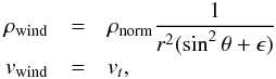 (4)where
ϵ = 0.01 is added to avoid the singularity at the pole
(θ = 0) (Lee et al. 2001).
vt is the terminal velocity of the wind, and
ρnorm is related to the wind mass-loss rate (rate at which
the wind carries matter from the protostar, Ṁwind) by mass
conservation,
(4)where
ϵ = 0.01 is added to avoid the singularity at the pole
(θ = 0) (Lee et al. 2001).
vt is the terminal velocity of the wind, and
ρnorm is related to the wind mass-loss rate (rate at which
the wind carries matter from the protostar, Ṁwind) by mass
conservation,  (5)We assumed that the
wind has a terminal velocity of 600 km s-1 (similar to Cunningham et al. 2005). The values for the mass-loss rate were chosen
to match the values found by Beuther et al. (2004).
Parameters for the wind are listed in Table 1.
(5)We assumed that the
wind has a terminal velocity of 600 km s-1 (similar to Cunningham et al. 2005). The values for the mass-loss rate were chosen
to match the values found by Beuther et al. (2004).
Parameters for the wind are listed in Table 1.
In principle, both the mass-loss rate of the wind and the density distribution of the envelope should evolve during the star formation process. However for simplicity, we only considered an envelope with a fixed density distribution and a wind with a fixed mass-loss rate. In practice, the timescale for local collapse is proportional to ρ− 1/2. Therefore, the central region where the protostars form evolves faster than the outer envelope, the density structure of the envelope evolves more slowly than the evolution of the wind mass-loss rate during the lifetime of the outflow.
2.2. Shape of the outflow cavity
The shape of the outflow cavity is determined by the balance of the ram-pressure of the
wind and the pressure of the envelope perpendicular to the outflow cavity wall (see Fig.
1). The magnitude of pwind
is  , and the magnitude
of the ram-pressure vector penvelope is
, and the magnitude
of the ram-pressure vector penvelope is
 . Projected
perpendicular to the edge of the outflow cavity, the magnitude of the wind pressure is
| pwind|sinφ and the magnitude of the
envelope pressure is | penvelope | (Fig. 1). The pressure balanceperpendicular to the wall of the outflow
cavity can then be written as
. Projected
perpendicular to the edge of the outflow cavity, the magnitude of the wind pressure is
| pwind|sinφ and the magnitude of the
envelope pressure is | penvelope | (Fig. 1). The pressure balanceperpendicular to the wall of the outflow
cavity can then be written as  (6)Along the cavity wall, no
pressure balance is established, and the wind contributes its momentum to the outflow (see
Sect. 2.3).
(6)Along the cavity wall, no
pressure balance is established, and the wind contributes its momentum to the outflow (see
Sect. 2.3).
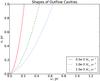 |
Fig. 2 Shapes of outflow cavities calculated for models with different wind mass-loss rates. The parameters are taken from Table 2. See Sect. 2.2 for details. |
Here we used cylindrical coordinates (ω,φ,z) for convenience. The polar
angle θ is specified as (Fig. 1)
 (7)and the angle
between the cavity wall and the z axis is specified as
(7)and the angle
between the cavity wall and the z axis is specified as  (8)This gives a value
φ of (Fig. 1)
(8)This gives a value
φ of (Fig. 1)  (9)Combining Eqs.
(6)−(9) gives
(9)Combining Eqs.
(6)−(9) gives  (10)Equation (10) determines the shape of the outflow
cavity. It is a first-order differential equation and can be solved numerically. We
imposed the boundary condition ω = 4.5 × 1015 cm at
z = 0, which is similar to those used by Parkin et al. (2009). The results are not sensitive to the choice of
this boundary condition.
(10)Equation (10) determines the shape of the outflow
cavity. It is a first-order differential equation and can be solved numerically. We
imposed the boundary condition ω = 4.5 × 1015 cm at
z = 0, which is similar to those used by Parkin et al. (2009). The results are not sensitive to the choice of
this boundary condition.
In deriving Eq. (10), we have neglected the effect of centrifugal force. As will be shown in Appendix A, centrifugal force is not significant in our case.
Using Eq. (10), we calculated the shapes of the outflow cavities for winds of different mass-loss rates. The results are shown in Fig. 2. It is clear that the opening angle of the outflow depends on the strength of the wind: a stronger wind leads to a less collimated outflow.
Observationally, the opening angle of the outflow evolves during the evolution of the protostar (Arce & Sargent 2006; Beuther & Shepherd 2005). This is interpreted as the evolution of the wind-envelope interaction (Arce & Sargent 2006). However, according to the widely accepted wind-driven shell model, the opening angle of the outflow should be fixed as the wind collimation is fixed and the density structure of the envelope does not evolve much (Lee et al. 2001). How the evolution of the wind-envelope interaction changes the collimation of the outflow is thus unclear.
According to our model, the outflow opening angle is determined by the force balance between the wind and the envelope. With the wind strength increases or the envelope becomes less turbulent, the opening angle of the outflow becomes larger, and the outflow tends to decollimate. Our model provides a quantitative explanation of the de-collimation of the outflow in the context of the wind-envelope interaction.
Turbulence in the envelope plays a vital role in our model: the shape of the outflow cavity is determined by the hydrostatic balance between the wind and the envelope, and an increase in the strength of the wind can decrease the collimation of the outflow, while an increase of the turbulence in the envelope can increase the collimation of the outflow. Turbulence helps to collimate the outflow.
2.3. Mass entrainment of the outflow layer
As discussed in Sect. 1, the growth of the outflow depends on the way matter is entrained into it.
The key parameter that characterizes the mass entrainment process is the local mass
entrainment rate, which is the amount of matter entrained per given time interval per
surface area. The entrainment rate ṁ can therefore be defined as
 (11)where
Mentrained is the amount of gas entrained, ds represents the
unit surface area and dt represents the time interval. The entrainment rate depend on the
density and the velocity involved in the entrainment process. Therefore, the general form
of the entrainment rate can be formulated as
(11)where
Mentrained is the amount of gas entrained, ds represents the
unit surface area and dt represents the time interval. The entrainment rate depend on the
density and the velocity involved in the entrainment process. Therefore, the general form
of the entrainment rate can be formulated as
 (12)where
cs, σturb and
vshear are the sound speed, turbulent speed and the velocity
difference between the shearing layer and the envelope, and
ρenvelope is the density of the envelope.
(12)where
cs, σturb and
vshear are the sound speed, turbulent speed and the velocity
difference between the shearing layer and the envelope, and
ρenvelope is the density of the envelope.
The factor fentrainment takes into account the effect of different speeds on the entrainment rate, and has the dimension of the velocity. In our case, the relative speed between the outflow and the envelope vshear is much higher than the velocity dispersion of the envelope σturb, and σturb is higher than the sound speed (vshear ≫ σturb > cs).
The entrainment process is driven by the shearing motion and limited by the transport
properties of the medium. The shearing motion is characterized by
vshear and the transport process is characterized by
σturb and cs. As
vshear ≫ σturb, the entrainment
rate is limited by the transport and is determined by a combination of
σturb and cs. In a turbulent
medium, turbulence dominates the transport. Therefore, in our model,
fentrainment is determined by turbulence. We thus take
 (13)where
α is a dimensionless factor that characterizes the efficiency of the
entrainment process. We therefore parametrized the entrainment rate in the presence of
turbulent motion as
(13)where
α is a dimensionless factor that characterizes the efficiency of the
entrainment process. We therefore parametrized the entrainment rate in the presence of
turbulent motion as  (14)where
σturb is the characteristic velocity of turbulent motion in
the medium. We assume α = 0.1 in this work.
(14)where
σturb is the characteristic velocity of turbulent motion in
the medium. We assume α = 0.1 in this work.
Historically, turbulent mixing has long been proposed as a mean of entraining mass into the outflow (e.g. Canto & Raga 1991; Watson et al. 2004). However, these models are doubted because the entrainment rate is far too small to account for the actual mass the outflow (Churchwell 1997). Realizing the importance of turbulence for enhancing the mass and momentum transport, we here propose that the argument by Churchwell (1997) no longer holds in our cases because turbulent mixing can be significantly enhanced when the ambient medium is turbulent.
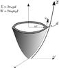 |
Fig. 3 Cartoon illustrating the geometry of the outflow layer and the definition of physical quantities in Sect. 2.4. |
2.4. Mass and momentum conservation in the entrainment layer
Based on the assumption that the outflow gas is the entrained envelope material, we
formulate the equations that govern the evolution of the outflow. The geometry of the
outflow is illustrated in Fig. 3. We defined the
x-axis to be along the wall of the outflow cavity and
vx as the average velocity of the outflow
along the x-axis. By doing this, our x-axis is no longer
a straight line. We used this construction for simplicity. ω is the same
as illustrated in Fig. 1, which gives a circumference
lc of
 (15)In Fig. 3, ρ is the average density and
d is the geometrical thickness of the outflow layer. In our case, the
outflow is geometrically thin (d ≪ l).
(15)In Fig. 3, ρ is the average density and
d is the geometrical thickness of the outflow layer. In our case, the
outflow is geometrically thin (d ≪ l).
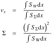
Σ is the integrated density, which is defined as
 (16)and
\begin{lxirformule}$W$\end{lxirformule} is the integrated momentum, which is defined as
(16)and
\begin{lxirformule}$W$\end{lxirformule} is the integrated momentum, which is defined as
 (17)where
vx is the average outflow velocity along
the outflow wall. Note that here d is introduced for convenience. At a
given position, we calculated Σ and W first. d can then
be evaluated as d = Σ/(2πωρ).
(17)where
vx is the average outflow velocity along
the outflow wall. Note that here d is introduced for convenience. At a
given position, we calculated Σ and W first. d can then
be evaluated as d = Σ/(2πωρ).
The equations of motion of the outflow layer describe the conservation of the mass and
the momentum, 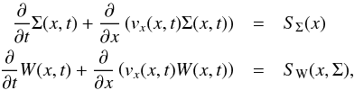 (18)where
W = vxΣ.
(18)where
W = vxΣ.
To solve it, we need the initial conditions Σ(x,t = 0) and W(x,t = 0).
We still need to specify the source terms SΣ and
SW. According to the geometry in Fig. 1, SΣ can be expressed as the sum of the
mass flow from the wind and the mass flow from the envelope,  (19)where
  (20)and according to Eq.
(14),
(20)and according to Eq.
(14),  (21)Here,
SΣwind ≪ SΣenvelope. Most of the
mass in the outflow comes from the envelope.
(21)Here,
SΣwind ≪ SΣenvelope. Most of the
mass in the outflow comes from the envelope.
SW is the source term for the integrated momentum.
SW consists of the momentum injection by the wind, as well
as the change of the momentum due to gravity. SW can then be
expressed as,  (22)where
g = GM∗/r2cosφ
is the acceleration due to gravity. Here, M∗ is the stellar
mass (10 M⊙), and cosφ comes from projecting
the gravity onto the wall of the outflow cavity. β is the wind
efficiency. It characterizes the efficiency with which the mixing layer absorbs mass and
momentum from the wind. We took 0.3 as its fiducial value.
(22)where
g = GM∗/r2cosφ
is the acceleration due to gravity. Here, M∗ is the stellar
mass (10 M⊙), and cosφ comes from projecting
the gravity onto the wall of the outflow cavity. β is the wind
efficiency. It characterizes the efficiency with which the mixing layer absorbs mass and
momentum from the wind. We took 0.3 as its fiducial value.
2.5. Local linear growth regime
Here we make an order-of-magnitude analysis of Eqs. (18). The first terms are the transient terms
 . The
second terms are the advection terms,
. The
second terms are the advection terms,  , and the third terms are
the source terms SP. Here, P
can be either Σ or W. If the outflow has initial mass and momentum
distribution P0 = Σ0
orW0, the mass/momentum accumulation timescales can be
written as
, and the third terms are
the source terms SP. Here, P
can be either Σ or W. If the outflow has initial mass and momentum
distribution P0 = Σ0
orW0, the mass/momentum accumulation timescales can be
written as  (23)and the advection
timescales can be written as
(23)and the advection
timescales can be written as  (24)Here, L
is the physical scale of the outflow, which is about 1 parsec.
(24)Here, L
is the physical scale of the outflow, which is about 1 parsec.
The mass/momentum accumulation timescale is dependent on the initial mass and momentum Σ0 and W0. If the majority of the mass and momentum of the outflow comes from the turbulence mixing process, Σ0 and W0 should be insignificant, therefore taccumulation is expected to be very short. Because we lack the knowledge on the initial mass and momentum distribution of the outflow, we assumed that the majority of the outflow mass and momentum comes from the turbulence mixing process. This assumption is valid as long as the outflow age is larger than the accumulation timescale taccumulation (Eq. (23)) is long. We studied the behaviour of Eqs. (18) by analysing the importance of different terms. For simplicity, we neglected the momentum added to the outflow due to self-gravity, therefore W(x,Σ) in Eqs. (18) can be approximated as W(x).
The advection timescale tadvection is the time required for
matter to travel throughout the outflow. If the outflow has an age of
toutflow, the transient term is
 (25)and the advection
term is
(25)and the advection
term is  (26)If we take the ratio
between the advection term and the transient term, we have
(26)If we take the ratio
between the advection term and the transient term, we have
 (27)where by definition
tadvection = L/v.
In our typical case, toutflow = 1 × 10⁴ yr and
tadvection ~ L/vx ~ 1pc/30 kms-1 ~ 1 × 10⁵ yr.
toutflow < tadvection,
therefore advection is not important in the whole outflow. In this case, the advection
effect can smooth out the density variations at the small scale, but can not alternate the
structure of the whole outflow significantly. This is also true for the outflow from the
class 0 low-mass protostars (Arce et al. 2007).
(27)where by definition
tadvection = L/v.
In our typical case, toutflow = 1 × 10⁴ yr and
tadvection ~ L/vx ~ 1pc/30 kms-1 ~ 1 × 10⁵ yr.
toutflow < tadvection,
therefore advection is not important in the whole outflow. In this case, the advection
effect can smooth out the density variations at the small scale, but can not alternate the
structure of the whole outflow significantly. This is also true for the outflow from the
class 0 low-mass protostars (Arce et al. 2007).
If the age of the outflow is small
(toutflow ≪ tadvection), as it
is most cases, we can neglect the advection terms in Eqs. (18), therefore we have  The
surface density of the outflow can then be calculated as
The
surface density of the outflow can then be calculated as  (30)and the velocity of
the outflow can be calculated as
(30)and the velocity of
the outflow can be calculated as  (31)In this case, the
velocity profile of the outflow is fixed and the surface density of the outflow grows
linearly with time.
(31)In this case, the
velocity profile of the outflow is fixed and the surface density of the outflow grows
linearly with time.
2.6. Advection-term-dominated regime
For the aged low-mass outflows (e.g outflows with t ~ 107yr),
we have toutflow ~ tadvection, and
the advection effect can alter the mass distribution of the outflow significantly.
Neglecting the transient terms in Eqs. (18), we have  hence
hence
 (34)Here,
both the velocity and the surface density exhibit stationary profiles. By comparing Eqs.
(30) and (31) with Eq. (34), we
find that when the outflow age is high, the advection term dominates the transient term,
which prevents the outflow surface density from growing to infinity.
(34)Here,
both the velocity and the surface density exhibit stationary profiles. By comparing Eqs.
(30) and (31) with Eq. (34), we
find that when the outflow age is high, the advection term dominates the transient term,
which prevents the outflow surface density from growing to infinity.
2.7. Role of gravity
Here we consider the role of the gravity term in the structure of the outflow. According
to Eq. (22), the contribution of gravity
is quantified by the ratio 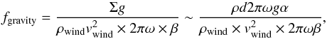 (35)where
d = σtα is used. Here, d is the
thickness of the outflow, α is the entrainment efficiency,
σ is the velocity dispersion of the envelope and t is
the outflow age. From this we have
(35)where
d = σtα is used. Here, d is the
thickness of the outflow, α is the entrainment efficiency,
σ is the velocity dispersion of the envelope and t is
the outflow age. From this we have
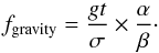 (36)Here,
σ is the velocity dispersion of the envelope, t is the
age of the outflow, and
g ~ GM∗/r2
is the local gravity. Since g ~ r-2, gravity
will be important at regions close to the protostar, and it will be important when the
mass of the outflow has grown significantly.
(36)Here,
σ is the velocity dispersion of the envelope, t is the
age of the outflow, and
g ~ GM∗/r2
is the local gravity. Since g ~ r-2, gravity
will be important at regions close to the protostar, and it will be important when the
mass of the outflow has grown significantly.
Considering the inner region of the outflow, we have M∗ = 10 M⊙, r = 0.1pc and t = 104yr. Therefore, fgravity ~ 10-2 and the gravity from the protostar is negligible. However, at regions closer to the protostar, gravity must play an important role in slowing down the outflow.
2.8. Numerical results
To illustrate how the mass and the momentum of the outflow grows with time, we assume a
static envelope and a wind with a constant mass-loss rate and followed the evolution of
the entrainment layer by solving Eqs. (18)−(22) numerically. The cavity
shapes are calculated in Sect. 2.2. At
x = 0, we imposed 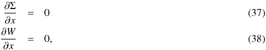 and
set the initial condition so that
and
set the initial condition so that  where
Δt0 = 100yr. The equations are solved using FiPy (J. E.
Guyer, D. Wheeler & J. A. Warren)1.
where
Δt0 = 100yr. The equations are solved using FiPy (J. E.
Guyer, D. Wheeler & J. A. Warren)1.
We are mainly interested in the transient-term-dominated regime, since because this regime is relevant to all high-mass protostellar outflows and the majority of the young low-mass protostellar outflows.
In Fig. 4, we plot the results from our calculations for a realistic 104yr outflow and unrealistically old 107yr outflow. In our 104yr outflow, the numerical solution agrees quite well with the analytical solutions (Sect. 2.5). At small radius, the numerical solutions show lower velocity. This is because the matter in regions close to the protostar is slowed down by the gravity from the protostar.
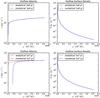 |
Fig. 4 Velocity and surface density distribution of the outflow calculated by solving Eqs. (18). The blue lines are the numerical results and the red lines are results calculated by assuming the local conservation of energy and momentum (Sect. 2.5). The upper panels are the results for a 104yr outflow. The lower panels are the results for an unrealistically old (107yr) outflow. At smaller radii, the deviation of the numerical solutions from the analytical solutions are caused by the gravity term in Eq. (22). |
We also plot the results of an outflow with an unrealistically long lifetime of 107yr. Because here gravity plays a much more significant role in slowing down the outflow (Sect. 2.7), the velocity of the outflow at the central part of the outflow becomes much lower.
In most cases, the effect of gravity is negligible in large portions of the outflow, the analytical solutions can be taken as good approximations to the structure of the outflow. However, it is difficult for the outflow to enter the advection-dominated regime, since here gravity tends to dominate the velocity structure of the outflow and to slow down the outward motion before advection is able to change the structure of the whole outflow significantly.
The final state we obtained from solving the equations of mass and momentum conservation in the local linear growth regime is representative of the real structure of the outflow, as long as the mass and momentum added to the outflow is much larger than the initial mass and momentum of the outflow. If the strength of the wind or the structure of the envelope changed during the evolution of the system, the final state of the outflow will change accordingly. Therefore, the system will evolve towards a new state, and the time for this evolution to take place is again the accumulation timescale (Eq. (23)). The older the outflow becomes, the more difficult it is for the outflow to relax to the new state.
In our present work, we assumed that the wind and envelope remain stationary. Our solution is valid when the structure of the wind and the structure of the envelope change slowly. Since detailed observations of the way in which the wind and envelope evolve are currently unavailable, we assume this simplicity. If the wind and the envelope both evolve significantly, it is still possible to calculate the structure of the outflow by making some modifications to the framework presented.
2.9. Structure of the entrainment layer
To fully specify the structure of the outflow, we need to know the structure of the entrainment layer. The gas motion inside the entrainment layer is dominated by turbulence, and its velocity can be expressed as the sum of a mean component and a fluctuating component (Reynolds 1895). There are many experiments and numerical simulations that study the structure of such a mixing layer (e.g. Champagne et al. 1976; Bell & Mehta 1990; Rogers & Moser 1994), from which we obtained the structures of the mean velocity and the fluctuating (random) velocity, and parametrized them.
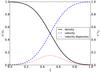 |
Fig. 5 Density and velocity structure of the entrainment layer. The (black) solid line denotes the density structure (Eq. (41)), the (blue) dashed line denotes the velocity structure (Eq. (42)), and the (red) dotted line denotes the structure of the fluctuating velocity (Eq. (44)). ξ is defined in Eq. (43). |
We found that the structure of the entrainment layer is universal and can be represented in a simple parametrized way. We fitted the mean density, the mean velocity and the turbulent velocity structures of Rogers & Moser (1994), and applied the fitting formula to our case.
The fitted density and mean velocity distributions take the forms of 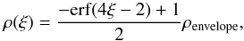 (41)and
 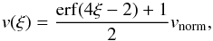 (42)where erf is the error
function, and ξ is defined as
(42)where erf is the error
function, and ξ is defined as  (43)d
is defined as
d = Σ /ρenvelope, and
vnorm = 5 × vx
due to the normalization requirement.
(43)d
is defined as
d = Σ /ρenvelope, and
vnorm = 5 × vx
due to the normalization requirement.
The distribution of the fluctuating velocity of the entrainment layer takes the form
 (44)where
vturb_norm = 0.15 × vnorm.
Figure 5 shows the structure of density, mean
velocity, and fluctuating velocity inside the entrainment layer.
(44)where
vturb_norm = 0.15 × vnorm.
Figure 5 shows the structure of density, mean
velocity, and fluctuating velocity inside the entrainment layer.
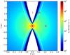 |
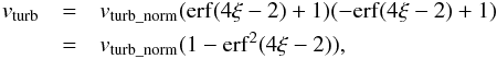
Fig. 6 Density structure of the outflow. Region I represents the inner cavity blown by the wind, region II represents the envelope, and region III represents the outflow layer. The wind mass-loss rate is 1.5 × 10⁻³M⊙yr-1. The thickness of the entrainment layer has been scaled up by a factor of 30 for clarity. |
Figure 6 shows the density distribution of our model, from which the entrainment layer can be identified as the region between the outflow cavity and the envelope.
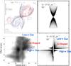 |
Fig. 7 Comparison between the observations by Qiu et al. (2009) and the predictions from our wind-driven turbulent entrainment model. The upper left panel shows the morphology of the outflow observed by Qiu et al. (2009), the lower left panel shows the position-velocity structure of the observed outflow. The upper right panel shows the morphology of the outflow from our modelling, the lower middle panel shows the position-velocity structure of our outflow model cut along its major axis. The outflow model has a mass-loss rate of 1.0 × 10⁻³ M⊙yr-1 and an inclination angle of 50°. For both the observations (lower left panel) and our modelling (lower right panel), the U-shaped region is the region in the position-velocity diagram where the structure of the outflow exhibits a U shape, the Low-v gas region is the region where the gas has a relative small velocity at regions far from the protostar, and the High-v gas region is the region where the gas has a relatively high velocity in the close vicinity to the protostar. |
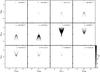 |
Fig. 8 CO(3−2) channel map of an outflow that has a mass-loss rate of 1.0 × 10⁻³M⊙yr-1 and an inclination angle of 50°. |
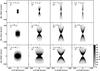 |
Fig. 9 Velocity-integrated CO(3−2) images of outflows from our model with different wind mass-loss rates and inclination angles. |
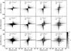 |
Fig. 10 CO(3−2) position-velocity diagram cut along the major axis of our outflow models with diferent wind mass loss rates and inclination angles. |
3. Observational tests
Observationally, molecular outflows are frequently mapped in the emission from rotational transitions of molecules such as CO and HCO+. These mapping observations can measure the intensity of the line emission from the outflow in the form of three-dimensional xyv (x-position-y-position-velocity) data cubes. CO is the most abundant and widespread molecule in the interstellar medium apart from the difficult-to-observe H2, and has been used to trace the bulk of molecular gas. CO observations (Lada 1985; Arce et al. 2007, and references therein) have revealed a diversity of molecular outflows, some of which show remarkably regular morphologies (e.g. Qiu et al. 2009).
Here we concentrated on modelling the emission from our outflows and studied the connection between the physical structure of the outflow models and the structure of our outflow models observed in a 3D data cube (e.g. Cabrit & Bertout 1986, 1990, 1992; Stahler 1994). To model the emission from the outflow, we need to know its dynamics and its abundance/excitation conditions. The dynamical structure of the outflow has been obtained in Sect. 2. However, the abundance and excitation are still uncertain: in regions close to the central protostar, the CO molecule can be photodissociated and cannot trace the gas anymore. The temperature of the outflow layer is determined by the balance between various heating and cooling processes, which are also uncertain. While these effects will influence the spacial and velocity distribution of the observed CO emission, the morphology of the outflow as well as its overall structure in the position-position and position-velocity spaces are relatively unchanged. Therefore we assume that the CO abundance is 10-4 relatively H2 and that the outflow entrainment layer has a constant kinematic temperature of ~100 K. In the following discussions, we focus on the overall morphology of the outflow in the position-position and position-velocity spaces.
For the velocity dispersion, velocity gradient and kinematic temperature from our model, we used a python version of RADEX (van der Tak et al. 2007) to calculate the population distribution of the CO molecule. We then used a ray-tracing code to calculate the line emission from our outflows. Our ray-tracing calculations were made with the help of LIME (Brinch & Hogerheijde 2010).
Figure 7 shows a comparison between our model and the observations by Qiu et al. (2009). We show the integrated image of the outflow and the position-velocity diagram of the outflow cut along the major axis. The integrated images of the outflow show a regular conical shape in both the observations and our modellings, and the position-velocity diagram of the outflows from observations and modellings show similar shapes. In regions close to the protostar, the observations show a velocity dispersion of about 20 km s-1. This velocity dispersion comes from a continuous distribution of emission and is consistent with observational studies (e.g. Qiu et al. 2011; Cyganowski et al. 2011).
We propose that this feature is one strong evidence for the existence of the entrainment layer. By looking at one position in the image, we integrate through the whole entrainment layer. In one line of sight, this produces a continuous distribution of fluids that move at different speeds (Fig. 5). Seen from the spectral line profile, we can always identify a broad component, since the line emission traces the distribution of the mass, and the mass distribution inside the entrainment layer is continuous.
On the other hand, the observation shown in Fig. 7 is difficult to understand in the context of the wind-driven shell model. In that model, the velocity of the outflow is proportional to the distance from the protostar and should vanish at close vicinity of the protostar, which is not observed (Fig. 7). Moreover, the outflow speed are high at regions far away from the protostar because only a high expansion velocity can make the gas move far. But in the observations we can still see low-velocity gas in regions far from the protostar.
Figure 8 shows a channel map of an outflow with a mass-loss rate of 1.0 × 10⁻³ M⊙yr-1 and an inclination angle of 50°. The inner part of the outflow is visible in most channels, implying a broad velocity spread at this location. This velocity spread is a direct consequence of the turbulent entrainment process.
Figures 9 and 10 show the calculated images and position-velocity diagrams of outflows from protostars with different mass-loss rates viewed at different inclination angles. The mass-loss rate takes values of 0.5, 1, 1.5, and × 10-3M⊙yr-1, the inclination angles values of 10°, 30°, and 50°. The calculated outflows exhibit a variety of morphologies. They also share some common characteristics: the outflow gas can reach a high velocity in regions close to a protostar; in regions far away from the protostar, there is still gas with low velocities. These features are natural outcomes of the entrainment process (Sect. 2.9) and can be observed under different circumstances.
4. Outflow entrainment as a universal process
Outflows are ubiquitously observed in a variety of situations, which include the formation of low-mass stars and high-mass stars, and the situation in which a wind blown by an AGN interacts and entrains the galactic-scale ambient gas (Alatalo et al. 2011; Tsai et al. 2012). Here we considered the possibility that these outflows have a common origin, in that all these outflows are formed through the interaction between the wind and the ambient gas in the form of turbulent entrainment.
In Sect. 4.1, using the turbulent core model of massive star formation (McKee & Tan 2002, 2003), we show that outflows from low and high-mass protostars can consistently be interpreted as resulting from an universal entrainment process. In Sect. 4.2, we derive universal scaling relations that can be used to estimate the mass and velocity of the outflows, and suggest that the AGN-driven outflows can be consistently explained in our model. In Sect. 4.3, using the insights obtained from the scaling analysis, we predict the existence of dwarf outflows in cluster-forming regions, and in Sect. 4.4 we discuss the self-similarity of our model.
4.1. Universal picture of protostellar outflows
As suggested by McKee & Tan (2002, 2003), the formation of high-mass stars can be viewed as a scaled-up version of the standard low-mass star formation theory from gas cores, where most of the pressure support is due to a combination of turbulence and magnetic fields instead of thermal pressure. In this picture, a high level of turbulence prevails in the high-mass star forming regions, causing significant turbulent ram-pressure of the ambient medium. The timescale for the formation of high-mass stars is short, and the accretion rate onto the high-mass protostar is much higher than in the low-mass case.
Our model of a turbulent entrainment outflow is self-similar in nature. By combining it with the self-similar star formation model, we can obtain a universal description of outflows from low and high-mass protostars.
Considering the fiducial case in McKee & Tan
(2003), the accretion rate onto the protostar can be estimated as  (45)where
m∗ is the current mass of the protostar,
m∗ f is the final mass of the protostar
when the accretion has been finished, and Σcl is the surface density of the
clump. High-mass star-forming regions are characterized by a high value of Σcl
(McKee & Tan 2003). The pressure of the
wind from the protostar can be estimated as
(45)where
m∗ is the current mass of the protostar,
m∗ f is the final mass of the protostar
when the accretion has been finished, and Σcl is the surface density of the
clump. High-mass star-forming regions are characterized by a high value of Σcl
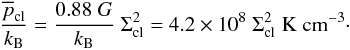
(McKee & Tan 2003). The pressure of the
wind from the protostar can be estimated as  (46)where
kB is the Boltzmann constant, and we assumed
ṁwind = 1/3 × ṁ∗
(Najita & Shu 1994, where
ṁ∗ is the total accretion rate onto the protostar) and
vwind = 600 km s-1. The average pressure of the
clump is expressed as (McKee & Tan 2003)
(46)where
kB is the Boltzmann constant, and we assumed
ṁwind = 1/3 × ṁ∗
(Najita & Shu 1994, where
ṁ∗ is the total accretion rate onto the protostar) and
vwind = 600 km s-1. The average pressure of the
clump is expressed as (McKee & Tan 2003)
 (47)For typical
parameters, the average pressure of the envelope
(47)For typical
parameters, the average pressure of the envelope  is similar to
the average pressure of the wind at 1pc, which is approximately the physical size of the
outflow. This justifies our suggestion that the ram-pressure of the wind and the
ram-pressure of the ambient medium are similar.
is similar to
the average pressure of the wind at 1pc, which is approximately the physical size of the
outflow. This justifies our suggestion that the ram-pressure of the wind and the
ram-pressure of the ambient medium are similar.
The collimation of the outflow is determined by the ratio between the turbulent
ram-pressure of the envelope and the ram-pressure of the wind. Stronger winds lead to
less-collimated outflows while more turbulent envelopes lead to highly collimated
outflows. To summarize these effects, we define the dimensionless
collimation parameter η of the outflow: 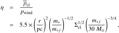 (48)with
larger η implying more collimated outflows.
(48)with
larger η implying more collimated outflows.
Equation (48) has several implications.
The ratio η is proportional to r-2, which means that the pressure of the envelope gradually dominates the pressure of the outflow tends to collimate the outflow with increasing distance from the protostar. This may explain why many outflows exhibit a re-collimated shape, that is, the opening angle of the outflow becomes smaller as we moves away from the protostar (e.g. L1157, Bachiller & Perez Gutierrez 1997).
Also,  , which
means that higher external pressure (stronger turbulence) leads to more collimated
outflows. This agrees with the results in Sect. 2.2, and
indicates that turbulence can collimate the outflow.
, which
means that higher external pressure (stronger turbulence) leads to more collimated
outflows. This agrees with the results in Sect. 2.2, and
indicates that turbulence can collimate the outflow.
Third, if the pressure of the clump Σcl is roughly constant, the more massive
the star is, the less collimated is the outflow. This is because η
depends on the final mass of the protostar,  .
The more massive the star, the stronger the wind it has. This stronger wind will push the
envelope and leads to a less collimated outflow. If several stars form in a clustered way
(Qiu et al. 2011), protostars of different mass
will share one common environment. We then expect that more massive protostars produce
less-collimated outflows.
.
The more massive the star, the stronger the wind it has. This stronger wind will push the
envelope and leads to a less collimated outflow. If several stars form in a clustered way
(Qiu et al. 2011), protostars of different mass
will share one common environment. We then expect that more massive protostars produce
less-collimated outflows.
4.2. Outflow mass and velocity
According to our model, the mass of the outflow is determined by the efficiency with
which the outflow entrains the envelope gas. Given the opening angle, the mass of the
outflow can be estimated as  (49)where
L is the physical scale of the outflow and
ρaverage and σaverage are the
average density and velocity dispersion, respectively. The average pressure of the
envelope is
(49)where
L is the physical scale of the outflow and
ρaverage and σaverage are the
average density and velocity dispersion, respectively. The average pressure of the
envelope is  (50)The momentum of
the outflow is determined by the amount of momentum injected by the wind and can be
estimated as
(50)The momentum of
the outflow is determined by the amount of momentum injected by the wind and can be
estimated as  (51)and the ram-pressure
of such a wind can be estimated as
(51)and the ram-pressure
of such a wind can be estimated as  (52)If the cavity
blown by the outflow is stable, the ram-pressure of the wind
pwind is expected to be similar to the turbulent
ram-pressure of the envelope, penvelope, and we have (from
Eqs. (50) and (52))
(52)If the cavity
blown by the outflow is stable, the ram-pressure of the wind
pwind is expected to be similar to the turbulent
ram-pressure of the envelope, penvelope, and we have (from
Eqs. (50) and (52))  (53)The outflow velocity is
then (Eqs. (49), (50), and (53))
(53)The outflow velocity is
then (Eqs. (49), (50), and (53)) 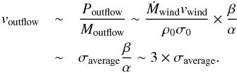 (54)In
the last step we inserted the numerical values of α and
β. The velocity of the outflow is several times higher than the
velocity dispersion of the envelope.
(54)In
the last step we inserted the numerical values of α and
β. The velocity of the outflow is several times higher than the
velocity dispersion of the envelope.
This fact can be understood as follows: If the wind and the envelope can establish hydrostatic equilibrium, then increasing turbulent velocity σ, the pressure of the wind has to scale according to σ2 to balance wind pressure. Therefore, the momentum injection of the wind scales as σ2. On the other hand, the mass supply of the outflow from the envelope in the form of the entrainment process only scales as σ1. The outflow velocity, which is estimated as P/M, scales as σ1.
These results outline one important property of the turbulent entrainment outflow, namely that the velocity of the outflow is higher than while still similar to the velocity dispersion of the ambient gas. This is independent of other parameters such as the strength of the wind, and is based only on the assumption that the wind and the envelope can establish hydrostatic equilibrium.
In recent Herschel-HIFI observations of high-J CO emission in low and high-mass star-forming regions (San Jose-Garcia et al. 2013), it was found that the velocity of the outflows (traced by the FWHM of the broad 12CO(10−9) line emission) is higher than while still similar to the velocity of the envelope (traced by the FWHM of the C18O(9−8) line). Also interesting is the fact that broader envelope line width is usually associated with broader outflow line width. This implies that the outflows from different regions share some physical similarities, and one possibility is that all these outflows come from the same entrainment process.
In a recently discovered AGN-driven outflow (Alatalo et al. 2011), the line width of the ambient gas (single-peaked central velocity component) is σenvelope ~ 100 km s-1, while the width of the broad line wing caused by the outflow activity is voutflow ~ 300 km s-1. Although velocity of the ambient gas and the velocity of the outflow are much higher than those of protostellar outflows, their ratio voutflow/σenvelope is about 3. This is similar to the ratio predicted in our model (Eq. (54)), which suggests that these outflows may be the outcome of the turbulent entrainment process working between the wind emitted by the central AGN and the galactic-scale ambient gas.
4.3. Dwarf outflows
As we have shown in Sect. 4.1, the emergence of an outflow depends on the pressure of the envelope and the pressure of the wind reaching a balance. This is not always true. If the wind from the protostars is not strong enough to blow away the envelope, we expect to see that the outflows have small spatial extent and are confined to small regions.
Such “dwarf” outflows may exist under several conditions. If several protostars form in a clustered way (e.g. Qiu et al. 2011), then the outflows from the low-mass protostars of different mass may be confined by the turbulence and appear as “dwarf outflow”. Alternatively, such “dwarf” outflows may exist at regions where the wind from the protostar is extremely weak (e.g. VeLLOs, Lee et al. 2009; Dunham et al. 2010). Studies of such “dwarf” outflows will help to gain insights into the interaction between the wind and the envelope in extreme cases.
4.4. Self-similarity of the model
We explored the self-similar properties of our model. Each model is characterized by
several parameters: a wind mass-loss rate Ṁ0, a turbulence
velocity σ0, a wind velocity
 , a density
ρ0, an outflow age t0, and the
entrainment parameters α0 and β0.
Our model is self-similar if when gravity is neglected. Here we derive the condition at
which the structure of another outflow characterized by a different set of parameters (
Ṁ1, σ1,
, a density
ρ0, an outflow age t0, and the
entrainment parameters α0 and β0.
Our model is self-similar if when gravity is neglected. Here we derive the condition at
which the structure of another outflow characterized by a different set of parameters (
Ṁ1, σ1,
 ,
ρ1, t1,
α1, and β1 ) can be obtained
from scaling of a different outflow.
,
ρ1, t1,
α1, and β1 ) can be obtained
from scaling of a different outflow.
The opening angle of the outflow is determined by the relative strength of the
ram-pressure of the wind and the turbulent ram-pressure of the envelope. For it to be
unchanged, we require 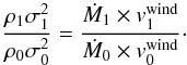 (55)If Eq. (55) is satisfied, the two outflows will have
the same shape. But the total amount of gas contained in the outflows and their velocity
are different. The amount of gas is proportional to the entrainment rate and proportional
to the outflow age, therefore
(55)If Eq. (55) is satisfied, the two outflows will have
the same shape. But the total amount of gas contained in the outflows and their velocity
are different. The amount of gas is proportional to the entrainment rate and proportional
to the outflow age, therefore 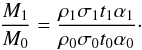 (56)As discussed in Sect.
4.2, the velocity of the outflow is proportional
to the velocity dispersion of the envelope,
(56)As discussed in Sect.
4.2, the velocity of the outflow is proportional
to the velocity dispersion of the envelope,  (57)These scaling
relations help us to put outflows with different masses and velocities into a common
picture.
(57)These scaling
relations help us to put outflows with different masses and velocities into a common
picture.
5. Conclusions
We studied the interaction between the wind from a protostar and the ambient gas in the form of turbulent mixing and proposed a wind-driven turbulent entrainment model for protostellar outflows. In the model, the wind from a protostar is in hydrostatic balance with the gas in the turbulent envelope, and the outflowing gas is completely contained in the turbulent entrainment layer that develops between the wind and the envelope. Turbulence in the ambient gas plays two roles in our model: first, turbulent motion determines the shape of the outflow (Sect. 2.2). Second, turbulence contributes to the mass growth of the mixing layer (Sect. 2.4). Our model is a universal one in that it can explain the outflows from both low and high-mass protostars (Sect. 4).
Our model can reproduce the geometry and kinematic structure of the observed outflows (Sect. 3, Figs. 7, 9 and 10). The main results from this study can be summarized as follows:
-
1.
At the physical scale of an outflow, the average ram-pressure ofwind is similar to the average ram-pressure of its envelope(Sect. 2.2, 4.1).
-
2.
The opening angle of the outflow is dependent on the pressure balance between the wind and the envelope, therefore it can evolve if the pressure of the wind or the pressure of the envelope changes (Sects. 2.2, 4.1).
-
3.
The ram-pressure of the wind tends to decollimate the outflow, the ram-pressure of the environment tends to collimate the outflow (Sects. 2.2, 4.1).
-
4.
At one given point in the observed image of the outflow, the emission has a wide spread in velocity (Sects. 3, Fig. 10). Both high-velocity gas in the close vicinity of the protostar and low-velocity gas in regions far from the protostar exist as the results of the turbulent entrainment process.
-
5.
If the outflow is formed through the turbulent entrainment process outlined here, the velocity spread of the outflow is expected to be about times the velocity spread of the ambient gas (Sect. 4.2). This is independent of the other physical parameters, such as the strength of the wind and the density of the region.
-
6.
In clustered star-forming regions, we expect a population of dwarf outflows that are confined by the pressure of their environment into small regions (Sect. 4.3).
Avaliable at http://www.ctcms.nist.gov/fipy/
Acknowledgments
We thank the anonymous referee for his/her insightful comments, which helped us to improve our draft. Guang-Xing Li is supported for this research through a stipend from the International Max Planck Research School (IMPRS) for Astronomy and Astrophysics at the Universities of Bonn and Cologne.
References
- Alatalo, K., Blitz, L., Young, L. M., et al. 2011, ApJ, 735, 88 [NASA ADS] [CrossRef] [Google Scholar]
- Arce, H. G., & Sargent, A. I. 2006, ApJ, 646, 1070 [NASA ADS] [CrossRef] [Google Scholar]
- Arce, H. G., Shepherd, D., Gueth, F., et al. 2007, Protostars and Planets V (Tucson: University of Arizona Press), 245 [Google Scholar]
- Bachiller, R., & Perez Gutierrez, M. 1997, ApJ, 487, L93 [NASA ADS] [CrossRef] [Google Scholar]
- Ballesteros-Paredes, J., Klessen, R. S., Mac Low, M.-M., & Vazquez-Semadeni, E. 2007, Protostars and Planets V (Tucson: University of Arizona Press), 63 [Google Scholar]
- Bell, J. H., & Mehta, R. D. 1990, AIAA Journal, 28, 2034 [NASA ADS] [CrossRef] [Google Scholar]
- Beuther, H., & Shepherd, D. 2005, in Cores to Clusters: Star Formation with Next Generation Telescopes, eds. M. S. N. Kumar, M. Tafalla, & P. Caselli (New York: Springer), 324, 105 [Google Scholar]
- Beuther, H., Schilke, P., Menten, K. M., et al. 2002, ApJ, 566, 945 [NASA ADS] [CrossRef] [Google Scholar]
- Beuther, H., Schilke, P., & Gueth, F. 2004, ApJ, 608, 330 [NASA ADS] [CrossRef] [Google Scholar]
- Biro, S., Canto, J., Raga, A. C., & Binette, L. 1993, Rev. Mex. Astron. Astrofis., 25, 95 [NASA ADS] [Google Scholar]
- Brinch, C., & Hogerheijde, M. R. 2010, A&A, 523, A25 [NASA ADS] [CrossRef] [EDP Sciences] [Google Scholar]
- Cabrit, S., & Bertout, C. 1986, ApJ, 307, 313 [NASA ADS] [CrossRef] [Google Scholar]
- Cabrit, S., & Bertout, C. 1990, ApJ, 348, 530 [NASA ADS] [CrossRef] [Google Scholar]
- Cabrit, S., & Bertout, C. 1992, A&A, 261, 274 [Google Scholar]
- Canto, J. 1980, A&A, 86, 327 [NASA ADS] [Google Scholar]
- Canto, J., & Raga, A. C. 1991, ApJ, 372, 646 [NASA ADS] [CrossRef] [Google Scholar]
- Canto, J., & Rodriguez, L. F. 1980, ApJ, 239, 982 [NASA ADS] [CrossRef] [Google Scholar]
- Champagne, F. H., Pao, Y. H., & Wygnanski, I. J. 1976, J. Fluid Mech., 74, 209 [NASA ADS] [CrossRef] [Google Scholar]
- Churchwell, E. 1997, ApJ, 479, L59 [NASA ADS] [CrossRef] [Google Scholar]
- Cunningham, A., Frank, A., & Hartmann, L. 2005, ApJ, 631, 1010 [NASA ADS] [CrossRef] [Google Scholar]
- Cyganowski, C. J., Brogan, C. L., Hunter, T. R., Churchwell, E., & Zhang, Q. 2011, ApJ, 729, 124 [NASA ADS] [CrossRef] [Google Scholar]
- Dunham, M. M., Evans, N. J., Bourke, T. L., et al. 2010, ApJ, 721, 995 [NASA ADS] [CrossRef] [Google Scholar]
- Fiege, J. D., & Henriksen, R. N. 1996, MNRAS, 281, 1038 [NASA ADS] [CrossRef] [Google Scholar]
- Keto, E., & Zhang, Q. 2010, MNRAS, 406, 102 [NASA ADS] [CrossRef] [Google Scholar]
- Krumholz, M. R., & McKee, C. F. 2005, ApJ, 630, 250 [NASA ADS] [CrossRef] [Google Scholar]
- Lada, C. J. 1985, ARA&A, 23, 267 [NASA ADS] [CrossRef] [Google Scholar]
- Larson, R. B. 1981, MNRAS, 194, 809 [NASA ADS] [CrossRef] [Google Scholar]
- Lee, C.-F., Mundy, L. G., Reipurth, B., Ostriker, E. C., & Stone, J. M. 2000, ApJ, 542, 925 [NASA ADS] [CrossRef] [Google Scholar]
- Lee, C.-F., Stone, J. M., Ostriker, E. C., & Mundy, L. G. 2001, ApJ, 557, 429 [NASA ADS] [CrossRef] [Google Scholar]
- Lee, C. W., Bourke, T. L., Myers, P. C., et al. 2009, ApJ, 693, 1290 [NASA ADS] [CrossRef] [Google Scholar]
- Lery, T., Henriksen, R. N., & Fiege, J. D. 1999, A&A, 350, 254 [NASA ADS] [Google Scholar]
- Li, Z.-Y., & Shu, F. H. 1996, ApJ, 472, 211 [NASA ADS] [CrossRef] [Google Scholar]
- Longmore, S. N., Pillai, T., Keto, E., Zhang, Q., & Qiu, K. 2011, ApJ, 726, 97 [NASA ADS] [CrossRef] [Google Scholar]
- Matzner, C. D. 2007, ApJ, 659, 1394 [NASA ADS] [CrossRef] [Google Scholar]
- Matzner, C. D., & McKee, C. F. 1999, ApJ, 526, L109 [NASA ADS] [CrossRef] [Google Scholar]
- McKee, C. F., & Holliman, II, J. H. 1999, ApJ, 522, 313 [NASA ADS] [CrossRef] [Google Scholar]
- McKee, C. F., & Tan, J. C. 2002, Nature, 416, 59 [NASA ADS] [CrossRef] [PubMed] [Google Scholar]
- McKee, C. F., & Tan, J. C. 2003, ApJ, 585, 850 [NASA ADS] [CrossRef] [MathSciNet] [Google Scholar]
- McLaughlin, D. E., & Pudritz, R. E. 1996, ApJ, 469, 194 [NASA ADS] [CrossRef] [Google Scholar]
- Mueller, K. E., Shirley, Y. L., Evans, II, N. J., & Jacobson, H. R. 2002, ApJS, 143, 469 [NASA ADS] [CrossRef] [Google Scholar]
- Najita, J. R., & Shu, F. H. 1994, ApJ, 429, 808 [NASA ADS] [CrossRef] [Google Scholar]
- Nakamura, F., & Li, Z.-Y. 2007, ApJ, 662, 395 [NASA ADS] [CrossRef] [Google Scholar]
- Offner, S. S. R., Lee, E. J., Goodman, A. A., & Arce, H. 2011, ApJ, 743, 91 [NASA ADS] [CrossRef] [Google Scholar]
- Ostriker, E. C. 1997, ApJ, 486, 291 [NASA ADS] [CrossRef] [Google Scholar]
- Parkin, E. R., Pittard, J. M., Hoare, M. G., Wright, N. J., & Drake, J. J. 2009, MNRAS, 400, 629 [NASA ADS] [CrossRef] [Google Scholar]
- Plume, R., Jaffe, D. T., Evans, II, N. J., Martin-Pintado, J., & Gomez-Gonzalez, J. 1997, ApJ, 476, 730 [NASA ADS] [CrossRef] [Google Scholar]
- Qiu, K., Zhang, Q., & Menten, K. M. 2011, ApJ, 728, 6 [NASA ADS] [CrossRef] [Google Scholar]
- Qiu, K., Zhang, Q., Wu, J., & Chen, H.-R. 2009, ApJ, 696, 66 [NASA ADS] [CrossRef] [Google Scholar]
- Ren, J. Z., Liu, T., Wu, Y., & Li, L. 2011, MNRAS, 415, L49 [NASA ADS] [CrossRef] [Google Scholar]
- Reynolds, O. 1895, Roy. Soc. London Philos. Trans. Ser. A, 186, 123 [Google Scholar]
- Rogers, M. M., & Moser, R. D. 1994, Phys. Fluids, 6, 903 [NASA ADS] [CrossRef] [Google Scholar]
- SanJose-Garcia, I., Mottram, J. C., Kristensen, L. E., et al. 2013, A&A, 553, A125 [NASA ADS] [CrossRef] [EDP Sciences] [Google Scholar]
- Shepherd, D. S., Watson, A. M., Sargent, A. I., & Churchwell, E. 1998, ApJ, 507, 861 [NASA ADS] [CrossRef] [Google Scholar]
- Shu, F. H., Ruden, S. P., Lada, C. J., & Lizano, S. 1991, ApJ, 370, L31 [NASA ADS] [CrossRef] [Google Scholar]
- Shu, F. H., Najita, J., Ostriker, E. C., & Shang, H. 1995, ApJ, 455, L155 [Google Scholar]
- Stahler, S. W. 1994, ApJ, 422, 616 [NASA ADS] [CrossRef] [Google Scholar]
- Tsai, A.-L., Matsushita, S., Kong, A. K. H., Matsumoto, H., & Kohno, K. 2012, ApJ, 752, 38 [NASA ADS] [CrossRef] [Google Scholar]
- van der Tak, F. F. S., Black, J. H., Schöier, F. L., Jansen, D. J., & van Dishoeck, E. F. 2007, A&A, 468, 627 [NASA ADS] [CrossRef] [EDP Sciences] [Google Scholar]
- Watson, C., Zweibel, E. G., Heitsch, F., & Churchwell, E. 2004, ApJ, 608, 274 [NASA ADS] [CrossRef] [Google Scholar]
Appendix A: Effect of centrifugal forces
As the outflowing gas moves along the cavity, it exerts a centrifugal force on its
surrounding. This effect has been considered in several previous works (e.g., Canto 1980; Canto
& Rodriguez 1980; Biro et al.
1993). The pressure produced by the centrifugal force can be estimated as
 (A.1)where
voutflow is the velocity of the outflow, κ
is the curvature of the outflow cavity, ρoutflow is the
density of the outflow, and d is the thickness of the outflow.
(A.1)where
voutflow is the velocity of the outflow, κ
is the curvature of the outflow cavity, ρoutflow is the
density of the outflow, and d is the thickness of the outflow.
The ram-pressure of the envelope is
 (A.2)In our
entrainment model, the density of the outflow is similar to the density of the envelope
ρoutflow ~ ρenvelope, and the
velocity of the outflow is several times the velocity dispersion of the envelope (Eq.
(54)). Therefore, the ratio between
centrifugal pressure and the pressure of the envelope is
(A.2)In our
entrainment model, the density of the outflow is similar to the density of the envelope
ρoutflow ~ ρenvelope, and the
velocity of the outflow is several times the velocity dispersion of the envelope (Eq.
(54)). Therefore, the ratio between
centrifugal pressure and the pressure of the envelope is  (A.3)where
R is the curvature radius. Here we are interested in making
order-of-magnitude estimations, and the effect of projection on the pressure is neglected.
Therefore we have
pwind ~ penvelope. In our
calculation, R is approximately the size of the outflow and
d is the thickness of the outflow. Here, we take advantage of the fact
that ρoutflow ~ ρenvelope and
voutflow ~ 3venvelope. It can be
seen that if d ~ R, centrifugal force will play an
important role in changing the shape of the outflow cavity. In our case, since
d ≪ R (Fig. 6,
note that the thickness of the outflow has been artificially scaled up for clarity, and in
fact our outflow layer is very thin compared with the size of the outflow), the influence
of centrifugal force is within a few percent and is therefore generally insignificant.
(A.3)where
R is the curvature radius. Here we are interested in making
order-of-magnitude estimations, and the effect of projection on the pressure is neglected.
Therefore we have
pwind ~ penvelope. In our
calculation, R is approximately the size of the outflow and
d is the thickness of the outflow. Here, we take advantage of the fact
that ρoutflow ~ ρenvelope and
voutflow ~ 3venvelope. It can be
seen that if d ~ R, centrifugal force will play an
important role in changing the shape of the outflow cavity. In our case, since
d ≪ R (Fig. 6,
note that the thickness of the outflow has been artificially scaled up for clarity, and in
fact our outflow layer is very thin compared with the size of the outflow), the influence
of centrifugal force is within a few percent and is therefore generally insignificant.
Our case is different from the case of Canto &
Rodriguez (1980) and Biro et al. (1993)
who found the centrifugal force to be important. This is because our entrainment process
conserves momentum and at the same time increases the mass of the outflow significantly,
and in Canto & Rodriguez (1980) and Biro et al. (1993) the entrainment process is
insignificant. To illustrate the effect of mass growth on the centrifugal force, we
consider a particle of mass m rotating along a circle of radius
R with velocity v. The centrifugal force can be
expressed as  (A.4)where
p is magnitude of the momentum of the particle. Here, it is quite clear
that when the momentum is conserved, the larger the mass, the weaker the centrifugal
force.
(A.4)where
p is magnitude of the momentum of the particle. Here, it is quite clear
that when the momentum is conserved, the larger the mass, the weaker the centrifugal
force.
In our case, the entrainment process conserves momentum, but the mass of the outflow has
been increased by a huge factor. Assuming pressure balance
pwind ~ penvelope, we have
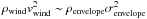 . The mass from
the wind is
mwind ~ ρwindvwindβ × ds,
where ds represents the surface area, and the mass from the envelope is
menvelope ~ α × ρenvelopeσenvelope × ds.
The ratio
menvelope/mwind
is
. The mass from
the wind is
mwind ~ ρwindvwindβ × ds,
where ds represents the surface area, and the mass from the envelope is
menvelope ~ α × ρenvelopeσenvelope × ds.
The ratio
menvelope/mwind
is 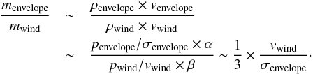 (A.5)Since
vwind ≫ σenvelope, the mass
growth from the entrainment process is huge, therefore the centrifugal force becomes
insignificant.
(A.5)Since
vwind ≫ σenvelope, the mass
growth from the entrainment process is huge, therefore the centrifugal force becomes
insignificant.
As the wind gas mixes with the ambient gas, the momentum of the system is conserved, but the mass of the system becomes much larger, therefore the centrifugal force becomes much smaller. This is because the momentum-conserving entrainment process increases the outflow mass significantly so that the centrifugal force is insignificant.
All Tables
All Figures
|
Fig. 1 Cartoon showing the basic structure of our model. The outflow (red region) lies between the wind and the envelope. Arrows (pwind and penvelope) denote the ram-pressure of the wind and the envelope. With wind we denote the cavity evacuated by the wind, with turbulent envelope we denote the turbulent envelope, and with outflow layer we denote the layer which contains the mixture of gas from the wind and gas from the envelope. |
| In the text | |
|
Fig. 2 Shapes of outflow cavities calculated for models with different wind mass-loss rates. The parameters are taken from Table 2. See Sect. 2.2 for details. |
| In the text | |
|
Fig. 3 Cartoon illustrating the geometry of the outflow layer and the definition of physical quantities in Sect. 2.4. |
| In the text | |
|
Fig. 4 Velocity and surface density distribution of the outflow calculated by solving Eqs. (18). The blue lines are the numerical results and the red lines are results calculated by assuming the local conservation of energy and momentum (Sect. 2.5). The upper panels are the results for a 104yr outflow. The lower panels are the results for an unrealistically old (107yr) outflow. At smaller radii, the deviation of the numerical solutions from the analytical solutions are caused by the gravity term in Eq. (22). |
| In the text | |
|
Fig. 5 Density and velocity structure of the entrainment layer. The (black) solid line denotes the density structure (Eq. (41)), the (blue) dashed line denotes the velocity structure (Eq. (42)), and the (red) dotted line denotes the structure of the fluctuating velocity (Eq. (44)). ξ is defined in Eq. (43). |
| In the text | |
|
Fig. 6 Density structure of the outflow. Region I represents the inner cavity blown by the wind, region II represents the envelope, and region III represents the outflow layer. The wind mass-loss rate is 1.5 × 10⁻³M⊙yr-1. The thickness of the entrainment layer has been scaled up by a factor of 30 for clarity. |
| In the text | |
|
Fig. 7 Comparison between the observations by Qiu et al. (2009) and the predictions from our wind-driven turbulent entrainment model. The upper left panel shows the morphology of the outflow observed by Qiu et al. (2009), the lower left panel shows the position-velocity structure of the observed outflow. The upper right panel shows the morphology of the outflow from our modelling, the lower middle panel shows the position-velocity structure of our outflow model cut along its major axis. The outflow model has a mass-loss rate of 1.0 × 10⁻³ M⊙yr-1 and an inclination angle of 50°. For both the observations (lower left panel) and our modelling (lower right panel), the U-shaped region is the region in the position-velocity diagram where the structure of the outflow exhibits a U shape, the Low-v gas region is the region where the gas has a relative small velocity at regions far from the protostar, and the High-v gas region is the region where the gas has a relatively high velocity in the close vicinity to the protostar. |
| In the text | |
|
Fig. 8 CO(3−2) channel map of an outflow that has a mass-loss rate of 1.0 × 10⁻³M⊙yr-1 and an inclination angle of 50°. |
| In the text | |
|
Fig. 9 Velocity-integrated CO(3−2) images of outflows from our model with different wind mass-loss rates and inclination angles. |
| In the text | |
|
Fig. 10 CO(3−2) position-velocity diagram cut along the major axis of our outflow models with diferent wind mass loss rates and inclination angles. |
| In the text | |
Current usage metrics show cumulative count of Article Views (full-text article views including HTML views, PDF and ePub downloads, according to the available data) and Abstracts Views on Vision4Press platform.
Data correspond to usage on the plateform after 2015. The current usage metrics is available 48-96 hours after online publication and is updated daily on week days.
Initial download of the metrics may take a while.