| Issue |
A&A
Volume 558, October 2013
|
|
|---|---|---|
| Article Number | L2 | |
| Number of page(s) | 4 | |
| Section | Letters | |
| DOI | https://doi.org/10.1051/0004-6361/201322576 | |
| Published online | 04 October 2013 | |
CO rotational line emission from a dense knot in Cassiopeia A
Evidence for active post-reverse-shock chemistry
1
Department of Earth and Space SciencesChalmers University of
Technology,
43992
Onsala,
Sweden
e-mail:
This email address is being protected from spambots. You need JavaScript enabled to view it.
2
Department Physik, Universität Basel, 4056
Basel,
Switzerland
3
Leiden Observatory, Leiden University,
PO Box 9513, 2300 RA
Leiden, The
Netherlands
4
Onsala Space Observatory, Chalmers University of
Technology, 43992
Onsala,
Sweden
5
Université de Toulouse, UPS-OMP, IRAP, 31028
Toulouse,
France
6
CNRS, IRAP, 9
Av. Colonel Roche, BP
44346, 31028
Toulouse Cedex 4,
France
7
SETI Institute, 189 N. Bernardo Ave, Mountain
View, CA
94043,
USA
8
Stratospheric Observatory for Infrared Astronomy,
NASA Ames Research Center, MS
211-3, Moffett
Field, CA
94035,
USA
Received: 30 August 2013
Accepted: 13 September 2013
Abstract
We report a Herschel⋆ detection of high-J rotational CO lines from a dense knot in the supernova remnant Cas A. Based on a combined analysis of these rotational lines and previously observed ro-vibrational CO lines, we find the gas to be warm (two components at ~400 and 2000 K) and dense (106−7 cm-3), with a CO column density of ~5 × 1017 cm-2. This, along with the broad line widths (~400 km s-1), suggests that the CO emission originates in the post-shock region of the reverse shock. As the passage of the reverse shock dissociates any existing molecules, the CO has most likely reformed in the past several years in the post-shock gas. The CO cooling time is similar to the CO formation time, therefore we discuss possible heating sources (UV photons from the shock front, X-rays, electron conduction) that may maintain the high column density of warm CO.
Key words: ISM: supernova remnants / submillimeter: ISM / ISM: individual objects: Cassiopeia A
Herschel is an ESA space observatory with science instruments provided by European-led Principal Investigator consortia and with important participation from NASA.
© ESO, 2013
1. Introduction
Stars with masses ranging from 8 to 30 M⊙ have lifetimes of only ~107 years (Woosley et al. 2002) before exploding as type II supernovae (SNe), and can thus enrich their local environments on a short timescale. Dust grains and molecules are produced in the ejected material (ejecta), despite the harsh physical conditions. Emission from CO and SiO molecules has been observed at infrared (IR) wavelengths in SN1987A some hundred days after the SN explosion (Danziger et al. 1987; Lucy et al. 1989; Roche et al. 1991), and in several other SNe (Kotak et al. 2005, 2006, 2009). These observations demonstrate that a rapid and efficient chemistry develops in the ejecta, and that molecular formation is a common occurrence in SNe (Lepp et al. 1990; Cherchneff & Sarangi 2011). CO and SiO have been observed in the ejecta of SN1987A (Kamenetzky et al. 2013), demonstrating that these molecules have survived up to 25 years after the SN explosion.
SNe are prime contenders for explaining the large dust masses in the early Universe, inferred from the reddening of background quasars and Lyman-α systems at high redshift (Pei et al. 1991; Pettini et al. 1994; Bertoldi et al. 2003), because efficient dust formation on short timescales is required. However, IR observations of SNe ~400 days post-explosion show dust masses ranging between 10-5 and 10-2M⊙ (e.g., Lucy et al. 1989; Sugerman et al. 2006; Szalai & Vinkó 2013), at least an order of magnitude too low to explain the observed high-z dust (Dwek et al. 2008). Larger dust masses have been observed in supernova remnants (SNRs), for example ~0.7 M⊙ of cool dust in the young remnant of SN1987A (Matsuura et al. 2011). Observations of the SNR Cas A imply ~0.025 M⊙ of warm dust (Rho et al. 2008), and ~0.075 M⊙ of cool dust (Barlow et al. 2010). However, these dust masses do not necessarily represent the net SN dust yields into the ISM, as the passage of a reverse shock might reprocess the dust grains.
When a SN explosion shock wave has swept up enough circumstellar and interstellar matter, a reverse shock forms and travels inward, decelerating and reprocessing the ejecta (Chevalier 1977). At the shock front the ejecta will be heated to >106 K, sputtering dust and dissociating molecules. However, the shock can be attenuated in dense knots in the ejecta, which mitigates its destructive effects there.
The 330-year-old SNR Cas A (D = 3.4 kpc) is the perfect laboratory for studying the effects of the reverse shock, because it is just beginning to reprocess the ejecta. Ro-vibrational CO emission has been detected in Cas A (Rho et al. 2009, 2012), in several (~20) small (<0.8″) knots coincident with the reverse shock. Such knots are reminiscent of the fast-moving knots (FMKs) seen in the optical (Fesen 2001). To determine the chemical and physical conditions in these knots, we used the Herschel PACS instrument to observe several high-J rotational CO lines toward the brightest CO knot in the remnant.
2. Observations
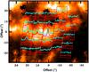 |
Fig. 1 PACS footprint, centered on RA 23:23:24.9 Dec +58:50:03.3, showing the spectra of CO J = 23–22 in blue and [O iii] 88 μm in red, overlaid on a Spitzer/IRAC image of the CO vibrational emission in Cas A. |
The Photodetector Array Camera and Spectrometer (PACS; Poglitsch et al. 2010) onboard the Herschel Space Observatory (Pilbratt et al. 2010) was used on 2012 June 11 to observe a single pointing in the northwest of Cas A (Fig. 1). PACS consists of a 5 × 5 array of spatial pixels (spaxels), each 9.4″× 9.4″ in size. We selected seven CO rotational transitions, between Jup = 14 and 38 for an even coverage of the CO ladder in the PACS spectral range. The observations were made using short-range spectroscopy scans with high spectral resolution (R = 1000–2700, ~100–300 km s-1). The [O iii] 88 μm transition was observed within the covered spectral range. Observations were done in chopping/nodding mode with a chop throw of 6′ to the north and south, well off the remnant.
The data were processed using the standard range-scan reduction pipeline, implemented in HIPE version 9.0.0 (Ott 2010). The CO J = 38–37 spectrum was marred by an artifact and thus discarded. A first-degree polynomial baseline was fit from line-free channels and subtracted. The final spectra correspond to the central spaxel after applying the standard PACS point-source correction to correct for flux spill-over into adjacent spaxels. PACS has an absolute flux accuracy of ~10% (PACS Observer’s Manual).
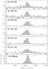 |
Fig. 2 CO and O iii emission lines in velocity (LSR), with Gaussian fits, extracted from the central PACS spaxel. Note that the flux density scale is different for the O iii line. |
Data of the CO and [O iii] lines extracted from the central spaxel.
3. Results
All the targeted CO lines were detected in the central PACS spaxel. The line profiles extracted from the central spaxel (Fig. 2) were fit with Gaussians (Table 1). The lines have an average radial velocity of –2740 km s-1, consistent with the velocity of the IR knot n2 (Rho et al. 2012, close to our target position), and are broad, with a deconvolved full width at half maximum of ~400 km s-1.
The integrated CO line fluxes were used to create a rotational diagram (Goldsmith & Langer 1999), as shown in Fig. 3. We adopted a source diameter of 0.5″ (much smaller than the spaxel size), consistent with the 0.8″ upper limit on the near-IR ro-vibrational CO source size (Rho et al. 2009) and optical observations of FMKs (Fesen 2001). Assuming local thermal equilibrium (LTE) conditions, we derived a column density of NCO = (4.1 ± 0.3) × 1017 cm-2 and a rotation temperature of Trot = 560 ± 20 K. This corresponds to a CO mass of ~5 × 10⁻⁶ M⊙ for the knot, which is independent of the assumed knot size, because NCO is inversely proportional to the knot size squared.
In the spectra of the full PACS footprint (Fig. 1) we see that the central spaxel emission has spilled over into the adjacent spaxels, because the point spread function is larger than the spaxel size. There is also some additional CO emission at the eastern edge of the footprint. This is most likely indicative of a second knot and not of extended CO emission, given the IR and optical evidence for a multitude of small, dense knots. Due to the increased uncertainty at the edge of the PACS footprint and the lower CO fluxes, we did not attempt to analyze this emission. In contrast to the CO emission, the emission of the [O iii] line is extended across the PACS footprint, which might be explained by its critical density, which is lower than that of the high-J CO lines.
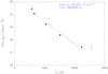 |
Fig. 3 CO excitation diagram, plotting ln (Nu/gu) vs. Eu. The column density, Ntot, and rotation temperature, Trot, and their uncertainties were calculated with a Monte Carlo method, excluding the last point; the blue line corresponds to the best-fit parameters. |
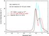 |
Fig. 4 Mid-IR AKARI spectrum reported by Rho et al. (2012) for knot n2 in Cas A is compared with models that have been convolved to the same resolution, 0.1125 μm. The black curve is the observed spectrum. The red curve is the computed spectrum for the same two-component non-LTE model that best describes the fluxes of the CO rotational lines, but scaled in intensity by a factor 1/16. The cyan curve represents the vibrational emission expected in strict LTE for the column density and temperature derived from the rotation diagram in Fig. 3, but scaled down by a factor of 10-4. The computed spectra include more than 4000 vibration-rotation lines, each of which has a width of 415 km s-1. |
4. Discussion
To investigate the physical conditions in the knot in more detail, we analyzed the CO excitation with the non-LTE radiative transfer code RADEX (van der Tak et al. 2007), assuming a uniform emitting region (i.e., constant density, temperature, and abundance). To fit all our rotational lines as well as the previously reported ro-vibrational emission from the same region (Rho et al. 2009, 2012), multiple temperature components are required: an ~400 K component and an additional ~2000 K component, containing about 15% of the CO, to explain the ro-vibrational fluxes (shown in Fig. 4). This hot component also contributes substantially to the high-J rotational lines. The multiple temperature components are suggestive of the structure of a post-shock cooling zone (Borkowski & Shull 1990).
The non-LTE analysis yields NCO ~ 5 × 1017 cm-2, similar to the rotation diagram result. The required density of the main collision partner is ~106 cm-3. Because the knot is expected to be oxygen-rich, with its strong [O iii] emission and similarity to optical FMKs, we consider oxygen to be the main collision partner in this knot. However, collisional rates with CO have only been studied with H/H2 and H2O as collision partners. Hence, these rates were used as proxies for the unknown O + CO collisional rates. The derived density differs by an order of magnitude depending on the chosen collision partner. On the other hand, the critical densities of the observed CO lines are ~106−7 cm-3, constraining the gas density to be fairly high. The RADEX analysis indicates that the observed CO lines are optically thin (τ < 10-2). Overall, the non-LTE analysis results are consistent with the simple rotational diagram analysis.
The high temperature and density of the CO along with the broad (~400 km s-1) lines suggests that the CO emission originates in a dense knot in the post-shock region of the reverse shock. In a dense knot, the reverse shock is attenuated due to energy conservation. Following Docenko & Sunyaev (2010), a 2000 km s-1 reverse shock will be slowed to 200 km s-1 when crossing a knot 100 times denser than the interclump medium. For a 200 km s-1 shock, the gas temperature at the shock front reaches some 107 K, and pre-existing molecules, including CO, will be destroyed. However, ongoing chemical modeling suggests that under the observed post-shock conditions, CO will reform on a timescale of tCO ~ 100 days through radiative association reactions (Biscaro & Cherchneff, in prep.).
Shock attenuation in dense knots also has implications for the survival of SN-produced dust. A slow shock may sputter <50% of the dust mass (Silvia et al. 2012), and the warm dense gas we see in the post-shock region is conducive to grain growth. Hence, some SN dust may survive the passage of the reverse shock in dense knots.
A minimum cooling flux, Λmin, can be estimated from the energy radiated by the observed [O iii] and CO lines in our knot. The [O iii] 88 μm line provides ~1 erg cm-2 s-1 of cooling, similar to that of the total rotational CO line emission, giving Λmin ~ 2 erg cm-2 s-1. Using a gas column density of 5 × 1019 cm-2, as explained below, we can calculate an approximate gas cooling time (tcool = NgaskBT/Λmin) of 70 days. This is similar to the CO formation timescale tCO ~ 100 days, indicating that a constant heating flux on the order of Λmin may be required to maintain the observed high column density of warm CO.
One heat source is the shock front itself, which emits UV photons. For a flux of Fo = no × vs (no = oxygen density; vs = shock velocity) oxygen atoms flowing into the shock, the total UV photon flux at the surface of the knot is 30 Fo photons cm-2 s-1 (Borkowski & Shull 1990, Table 11). With a typical photon energy of 20 eV, we derive a heating flux of ~2 erg cm-2 s-1, similar to Λmin. However, the penetration depth of the UV photons is only ~3 × 1017 cm-2 (Borkowski & Shull 1990), while the derived O iii column density is ~1019 cm-2. In addition, NCO ~ 5 × 1017 cm-2 implies a gas column density of at least 5 × 1019 cm-2, as the pre-shock CO abundance in such a knot is expected to be ~10-2 (Sarangi & Cherchneff 2013). Hence, the UV photons cannot penetrate the full gas column, and additional heating sources must be considered.
The reverse shock traveling through the tenuous inter-knot ejecta creates a hot plasma that will slowly cool through X-rays. Taking the average observed X-ray luminosity over the remnant, 5.5 × 1037 erg s-1 (Hartmann et al. 1997), with a typical photon energy of ~2 keV, we obtain an X-ray heating flux of 0.2 erg cm-2 s-1 at the knot. While the keV photons might ionize and heat a higher column density (~3 × 1019 cm-2) than the UV photons, the X-ray heating flux falls short of Λmin by an order of magnitude.
Heat conduction from the inter-knot hot, tenuous plasma into the dense knot might provide another heating source. The classical expression for heat conduction by electrons gives Q = K(T) dT/dr, where K(T) is approximately constant and ~6 × 10⁻⁷ × T5/2 erg s-1 K−7/2 cm-1 (Tielens 2005, p. 448–449). Setting the temperature gradient equal to T/δR with the temperature T = 107 K and the length scale δR given by the gas column density divided by the gas density, N/n = 5 × 1013 cm, we find an energy flux of ~4 × 10⁴ erg cm-2 s-1, which will be balanced by mass evaporation from the knot surface. The energy radiated away through the CO lines is then of little relevance for the energy budget. For the adopted parameters, the mean free path for electrons (~1012 cm) is short compared with the size scale for the temperature gradient (5 × 1013 cm), as required by the classical heat conduction expression. Though the heat flux conducted inward by electrons may be limited somewhat by magnetic fields, still heat conduction may be the key to maintaining the high column density of warm gas.
In conclusion, Herschel observations of rotational CO lines in a dense knot in Cas A indicate a high column density (NCO ~ 5 × 1017 cm-2) of warm (two components at ~400 and 2000 K) and dense (106−7 cm-3) gas in the post-shock region of the reverse shock. The passage of the shock
will dissociate any existing molecules and hence the CO has most likely been reformed recently, in the post-shock gas, providing evidence of an active chemistry in the post-reverse-shock region. The observed high column density of warm CO indicates that the cooling through CO (and ionic) lines is balanced by a constant heating flux. The diffuse X-ray flux is insufficient, and the UV photons from the shock front cannot penetrate the full gas column; accordingly, heat conduction by electrons may be required to maintain the temperature of the gas.
Herschel is an ESA space observatory with science instruments provided by European-led Principal Investigator consortia and with important participation from NASA.
Acknowledgments
S.W. and C.B. thank the ESF EuroGENESIS programme for financial support through the CoDustMas network.
References
- Barlow, M. J., Krause, O., Swinyard, B. M., et al. 2010, A&A, 518, 138 [Google Scholar]
- Bertoldi, F., Carilli, C. L., Cox, P., et al. 2003, A&A, 406, 55 [Google Scholar]
- Borkowski, K. J., & Shull, M. J. 1990, ApJ, 348, 169 [NASA ADS] [CrossRef] [Google Scholar]
- Cherchneff, I., & Sarangi, A. 2011, IAU Symp., 280, 22 [Google Scholar]
- Chevalier, R. 1977, ARA&A, 15, 175 [NASA ADS] [CrossRef] [Google Scholar]
- Danziger, I. J., Fosbury, R. A. E., Alloin, D., et al. 1987, A&A, 177, L13 [NASA ADS] [Google Scholar]
- Docenko, D., & Sunyaev, R. A. 2010, A&A, 509, 59 [Google Scholar]
- Dwek, E., Arendt, R. G., Bouchet, P., et al. 2008, ApJ, 676, 1029 [NASA ADS] [CrossRef] [Google Scholar]
- Fesen, R. A. 2001, ApJS, 133, 161 [NASA ADS] [CrossRef] [Google Scholar]
- Goldsmith, P. F., & Langer, W. D. 1999, ApJ, 517, 209 [NASA ADS] [CrossRef] [Google Scholar]
- Hartmann, D. H., Predehl, P., Greiner, J., et al. 1997, Nucl. Phys. A, 621, 83 [NASA ADS] [CrossRef] [Google Scholar]
- Kamenetzky, J., McCray, R., Indebetouw, R., et al. 2013, ApJ, 773, 34 [Google Scholar]
- Kotak, R., Meikle, P., van Dyk, S. D., et al. 2005, ApJ, 628, L123 [NASA ADS] [CrossRef] [Google Scholar]
- Kotak, R., Meikle, P., Pozzo, M., et al. 2006, ApJ, 651, L117 [NASA ADS] [CrossRef] [Google Scholar]
- Kotak, R., Meikle, W. P. S., Farrah, D., et al. 2009, ApJ, 704, 306 [NASA ADS] [CrossRef] [Google Scholar]
- Lepp, S., Dalgarno, A., & McCray, R. 1990, ApJ, 358, 262 [NASA ADS] [CrossRef] [Google Scholar]
- Lucy, L. B., Danziger, I. J., Gouiffes, C., & Bouchet, P. 1989, in Structure and Dynamics of the Interstellar Medium, IAU Colloq. 120, eds. G. Tenorio-Tagle, M. Moles, & J. Melnick, 164 [Google Scholar]
- Matsuura, M., Dwek, E., Meixner, M., et al. 2011, Science, 333, 1258 [NASA ADS] [CrossRef] [Google Scholar]
- Ott, S. 2010, ASP Conf. Ser., 434, 139 [Google Scholar]
- Pei, Y. C., Fall, S. M., & Bechtold, J. 1991, ApJ, 378, 6 [NASA ADS] [CrossRef] [Google Scholar]
- Pettini, M., Smith, L. J., Hunstead, R. W., & King, D. L. 1994, MNRAS, 394, 2266 [Google Scholar]
- Pilbratt, G., Riedinger, J., Passvogel, T., et al. 2010, A&A, 518, L1 [CrossRef] [EDP Sciences] [Google Scholar]
- Poglitsch, A., Waelkens, C., Geis, N., et al. 2010, A&A, 518, L2 [NASA ADS] [CrossRef] [EDP Sciences] [Google Scholar]
- Rho, J., Kozasa, T., Reach, W. T., et al. 2008, ApJ, 673, 271 [NASA ADS] [CrossRef] [Google Scholar]
- Rho, J., Jarrett, T. H., Reach, W. T., et al. 2009, ApJ, 693, 39 [Google Scholar]
- Rho, J., Onaka, T., Cami, J., & Reach, W. T. 2012, ApJ, 747, 6 [Google Scholar]
- Roche, P. F., Aitken, D. K., & Smith, C. H. 1991, MNRAS, 252, 39 [NASA ADS] [Google Scholar]
- Sarangi, A., & Cherchneff, I. 2013, ApJ, in press [Google Scholar]
- Silvia, D. W., Smith, B. D., & Shull, J. M. 2012, ApJ, 748, 12 [NASA ADS] [CrossRef] [Google Scholar]
- Sugerman, B. E. K., Ercolano, B., Barlow, M. J., et al. 2006, Science, 313, 196 [NASA ADS] [CrossRef] [PubMed] [Google Scholar]
- Szalai, T., & Vinkó, J. 2013, A&A 549, A79 [Google Scholar]
- Tielens, A. G. G. M. 2005, The Physics and Chemistry of the Interstellar Medium (Cambridge University Press) [Google Scholar]
- van der Tak, F. F. S., Black, J. H., Schier, F. L., et al. 2007, A&A, 468, 627 [NASA ADS] [CrossRef] [EDP Sciences] [Google Scholar]
- Woosley, S. E., Heger, A., & Weaver, T. A. 2002, RvMP, 74, 1015 [NASA ADS] [Google Scholar]
All Tables
All Figures
|
Fig. 1 PACS footprint, centered on RA 23:23:24.9 Dec +58:50:03.3, showing the spectra of CO J = 23–22 in blue and [O iii] 88 μm in red, overlaid on a Spitzer/IRAC image of the CO vibrational emission in Cas A. |
| In the text | |
|
Fig. 2 CO and O iii emission lines in velocity (LSR), with Gaussian fits, extracted from the central PACS spaxel. Note that the flux density scale is different for the O iii line. |
| In the text | |
|
Fig. 3 CO excitation diagram, plotting ln (Nu/gu) vs. Eu. The column density, Ntot, and rotation temperature, Trot, and their uncertainties were calculated with a Monte Carlo method, excluding the last point; the blue line corresponds to the best-fit parameters. |
| In the text | |
|
Fig. 4 Mid-IR AKARI spectrum reported by Rho et al. (2012) for knot n2 in Cas A is compared with models that have been convolved to the same resolution, 0.1125 μm. The black curve is the observed spectrum. The red curve is the computed spectrum for the same two-component non-LTE model that best describes the fluxes of the CO rotational lines, but scaled in intensity by a factor 1/16. The cyan curve represents the vibrational emission expected in strict LTE for the column density and temperature derived from the rotation diagram in Fig. 3, but scaled down by a factor of 10-4. The computed spectra include more than 4000 vibration-rotation lines, each of which has a width of 415 km s-1. |
| In the text | |
Current usage metrics show cumulative count of Article Views (full-text article views including HTML views, PDF and ePub downloads, according to the available data) and Abstracts Views on Vision4Press platform.
Data correspond to usage on the plateform after 2015. The current usage metrics is available 48-96 hours after online publication and is updated daily on week days.
Initial download of the metrics may take a while.