© ESO, 2013

1. Introduction

Recent spacecraft observations have revealed the necessity to refine the modeling of the transport of charged energetic particles to allow for strongly pitch-angle–anisotropic phase space distribution functions, which cannot be properly accounted for by the diffusion approximation. In addition to solar energetic particles (SEPs) in general, for which this requirement has been known for decades (Roelof 1969, for a review see Dröge 2000), other heliospheric particle populations were identified to exhibit such anisotropies. Examples are the so-called Jovian electron jets (Ferrando et al. 1993; Dunzlaff et al. 2010) and suprathermal ion species accelerated at interplanetary traveling shocks (le Roux & Webb 2012), as well as at the solar wind termination shock (Decker et al. 2005; Florinski et al. 2008; le Roux & Webb 2012).

Central to such a modeling refinement is the determination of the pitch-angle diffusion coefficient D_μμ that occurs in the Fokker-Planck transport equation (Schlickeiser 2002; Shalchi 2009). In general, one can distinguish at least three different methods of addressing this problem.

First, the wave number k-dependence of the turbulent power spectrum G(k) can be specified to derive analytical approximations for D_μμ. The quasi-linear theory (QLT) derived by Jokipii (1966) has been the standard theory, until it was realized that QLT is not only inaccurate but, in fact, invalid for some scenarios. For the example of isotropic turbulence, it has been known from both qualitative arguments (Fisk et al. 1974; Bieber et al. 1988) and detailed calculations (Tautz et al. 2006) that QLT cannot properly describe pitch-angle scattering, because it neglects 90° scattering and leads to infinitely large mean-free paths. This problem was remedied by the application of the second-order QLT (SOQLT, see Shalchi 2005; Tautz et al. 2008), which considers deviations from the unperturbed spiral orbits that were assumed in QLT.

Second, to allow for more complex turbulence properties and to validate the permissibility of the analytical perturbation theories, one can resort to test particle simulations in specified turbulent magnetic fields. By tracing particle trajectories, the mean square displacements and the associated diffusion parameters can be obtained. On the one hand, there have been successful attempts to confirm quasi-linear results (Qin & Shalchi 2009). On the other, such simulations have been employed to investigate the general behavior of pitch-angle scattering as described by the direct summation of multiple particle deflections (Lemons et al. 2009). Further examples of application of this method include the studies of the effects of structured (Laitinen et al. 2012) and balanced turbulence (Laitinen et al. 2013) on the particle transport, and consideration of inhomogeneous magnetic background fields (Tautz et al. 2011; Kelly et al. 2012).

Third, rather than entirely specifying the turbulent magnetic fields, one can perform direct numerical simulations to compute solutions to the magnetohydrodynamic equations, while the test-particle trajectories are still integrated as in the previous method. Such computations (see, e.g., Beresnyak et al. 2011; Spanier & Wisniewski 2011; Wisniewski et al. 2012) do not require assumptions regarding the turbulence spectrum that is seen by the energetic particles. They are, however, limited regarding the extent of the inertial range of the turbulence spectrum, owing to computational constraints. In the present study we, therefore, restrict ourselves to the first and second approaches.

We undertake a systematic comparison between analytical predictions of the Fokker-Planck coefficient of pitch-angle scattering and numerical simulations that are based on a Monte-Carlo code developed by one of us (Tautz 2010). In Sect. 2, the Monte-Carlo code Padian is introduced, which is used for all numerical simulations. In Sects. 3 and 4, basic properties of pitch-angle scattering and of the Fokker-Planck coefficient are presented, respectively. In Sect. 5, results from the numerical simulations are compared to estimations obtained from analytical scattering theories. Sect. 6 provides a summary and a discussion of the results.

2. Padian simulation code

For the numerical simulations, a Monte-Carlo code was used to compute the parallel diffusion coefficient of energetic particles for the turbulence model described above. A general description of the code and the underlying numerical techniques can be found elsewhere (Tautz 2010; Tautz & Dosch 2013). Specifically, the isotropic and the slab turbulence models were employed, which are defined via the wave vector of the (Fourier transformed) turbulent magnetic field with random orientation and aligned with the direction of the background magnetic field (i.e., the z axis), respectively. The corresponding generation of turbulent magnetic fields proceeded as (Tautz & Dosch 2013) $\mathit{\delta }{B}\mathrm{\left(}{r}\mathit{,t}\mathrm{\right)}\mathrm{=}\sum _{\mathit{n}\hspace{0.17em}\mathrm{=}\hspace{0.17em}\mathrm{1}}^{{\mathit{N}}_{\mathit{m}}}{{e}}_{\mathrm{\perp }}^{\mathrm{\prime }}\mathit{A}\mathrm{\left(}{\mathit{k}}_{\mathit{n}}\mathrm{\right)}\cos \left[{\mathit{k}}_{\mathit{n}}{\mathit{z}}^{\mathrm{\prime }}\mathrm{+}{\mathit{\beta }}_{\mathit{n}}\right]\mathit{,}$(1)where the wavenumbers k_n are distributed logarithmically in the interval , and β is a random phase angle.

The slab turbulence model is motived by Mariner 2 measurements, indicating that the solar wind is dominated by outward propagating Alfvénic turbulence (Belcher & Davis 1971; Tautz & Shalchi 2013). Together with a second, two-dimensional contribution, this gave rise to the composite turbulence model (Bieber et al. 1996; Matthaeus et al. 1990; Rausch & Tautz 2013). In numerical simulations, in contrast, Alfvénic modes exhibit a scale-dependent anisotropy consistent with the Goldreich-Sridhar (1994,1995) model. Nevertheless, the classic slab model remains attractive, especially for analytical investigations, thereby allowing one to isolate specific effects.

For the amplitude and the polarization vector, one has $\mathit{A}\mathrm{\left(}{\mathit{k}}_{\mathit{n}}\mathrm{\right)}\mathrm{\propto }\sqrt{\mathit{G}\mathrm{\left(}{\mathit{k}}_{\mathit{n}}\mathrm{\right)}}$ and ${{e}}_{\mathrm{\perp }}^{\mathrm{\prime }}\mathrm{·}{{e}}_{\mathit{z}}^{\mathrm{\prime }}\mathrm{=}\mathrm{0}$, respectively, with the primed coordinates determined by a rotation matrix with random angles so that ${k}\mathrm{\parallel }\hat{{e}}{}_{\mathit{z}}$ for slab modes and random k directions for isotropic modes. From the integration of the Newton-Lorentz equation for the particle motion, various diffusion coefficients can then be calculated by averaging over an ensemble of particles and by determining the mean square displacement. For example, the scattering mean free path in the direction parallel to the background magnetic field can be obtained as λ _∥  = (3/v)    ⟨ (Δz)² ⟩ /(2t) for large times (cf. Sect. 3).

For the minimum and maximum wavenumbers included in the turbulence generator, the following considerations apply: (i) the resonance condition states that there has to be a wavenumber k so that R_Lk ≈ 1, where R_L denotes the particle’s Larmor radius so that scattering predominantly occurs when a particle can interact with a wave mode over a full gyration cycle; (ii) the scaling condition requires that R_LΩ_relt < L_max, where Ω_rel = qB/(γmc) is the relativistic gyrofrequency and where L_max ∝ 1/k_min is the maximum extension of the system, which is given by the lowest wavenumber (for which one has k_min = 2π/λ_max, thereby proving the argument). In practice, the second condition determines the minimum wavenumber, while the first one determines the maximum wavenumber.

Here, values are chosen as k_minℓ₀ = 10^-4 and k_maxℓ₀ = 10⁴, where ℓ₀ is the turbulence bend-over scale (see Appendix A). The sum in Eq. (1)extends over N_m = 512 wave modes, which is sufficient (Tautz & Dosch 2013) and yet saves computation time. Furthermore, the maximum simulation time is determined as vt/ℓ₀ = 10¹ for low particle energies and 10² for high particle energies.

3. Pitch-angle scattering

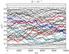Fig. 1 Pitch-angle cosine, μ = v ∥ /v as a function of the normalized time, τ = Ωt for a relative slab turbulence strength δB/B0 = 10-2. Four particles with initial pitch angles in the range 0.1 ≲ μ0 ≲ 0.8 are highlighted to guide the eye. (This figure is available in color in electronic form)

Perhaps the most important transport process of high-energy particles is represented by pitch-angle scattering, i.e., by stochastic variations in μ = cos∠(v,B₀) = v _∥ /v with range  [−1,1] , where ${{B}}_{\mathrm{0}}\mathrm{=}{\mathit{B}}_{\mathrm{0}}\hat{{e}}{}_{\mathit{z}}$ is the mean magnetic field and v is the particle velocity. This process is related to diffusion along the mean magnetic field, which is described by the parallel diffusion coefficient, κ _∥ , or the parallel mean free path, λ _∥  = (3/v)κ _∥ , which are also related to the cosmic ray anisotropy (Schlickeiser 1989; Shalchi et al. 2009).

The time evolution of the pitch angle is shown in Fig. 1 for a sample of typical single-particle trajectories (without any averaging process). It is indeed confirmed that particles with μ ≈  { 0, ± 1 }  almost retain their original pitch angle. However, scattering through 90° can occur, a fact that is not included in QLT. An introduction to analytical transport theories can be found, e.g., in Schlickeiser (2002) and Shalchi (2009).

3.1. General remarks

The usual definition of pitch-angle scattering can be found in the so-called Taylor-Green-Kubo (TGK) formalism (Taylor 1922; Green 1951; Kubo 1957; Shalchi 2011) as 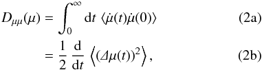$\begin{array}{ccc}{\mathit{D}}_{\mathit{\mu \mu }}\mathrm{\left(}\mathit{\mu }\mathrm{\right)}& \mathrm{=}& \int \begin{array}{}\mathrm{\infty }\\ \mathrm{0}\end{array}\mathrm{d}\mathit{t}\hspace{0.17em}⟨\mathit{\mu ̇}\mathrm{\left(}\mathit{t}\mathrm{\right)}\mathit{\mu ̇}\mathrm{\left(}\mathrm{0}\mathrm{\right)}⟩\\ & \mathrm{=}& \frac{\mathrm{1}}{\mathrm{2}}\hspace{0.17em}\frac{\mathrm{d}}{\mathrm{d}\mathit{t}}\hspace{0.17em}\mathrm{⟨}{\left(\mathit{\Delta \mu }\mathrm{\left(}\mathit{t}\mathrm{\right)}\right)}^{\mathrm{2}}\mathrm{⟩}\mathit{,}\end{array}$where the second line employs the definition Δμ(t) = μ(t) − μ(0). It can be shown (e.g., Shalchi 2011) that both versions agree with each other, if t is high enough that the expression becomes asymptotically time-independent.

The combination of diffusion (Fick 1855) and random walk (Chandrasekhar 1943) motivated the usual definition of the diffusion in terms of the mean-square displacement (e.g., Tautz 2012) κ =  ⟨ (Δx)² ⟩ /(2t), which can also be used for a third expression for D_μμ, namely 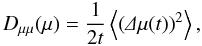${\mathit{D}}_{\mathit{\mu \mu }}\mathrm{\left(}\mathit{\mu }\mathrm{\right)}\mathrm{=}\frac{\mathrm{1}}{\mathrm{2}\mathit{t}}\mathrm{⟨}{\left(\mathit{\Delta \mu }\mathrm{\left(}\mathit{t}\mathrm{\right)}\right)}^{\mathrm{2}}\mathrm{⟩}\mathit{,}$(3)which is again valid if t is high enough. However, the formal limit t → ∞ is forbidden since |Δμ| cannot exceed a value of 2. For high enough times, D_μμ will always be dominated by the 1/t dependence, independent of the choice of the formula. Therefore, a meaningful, time-independent value for D_μμ can be obtained if and only if: (i) t is long enough that the initial conditions become insignificant; (ii) t is short enough that the behavior of D_μμ is not already dominated by the 1/t proportionality. This matter is further investigated in the second paper of this series (Tautz 2013).

3.2. Estimation of the critical time

Based on the preceding paragraph, we now calculate the critical time, t_max, by using QLT. This gives us an estimates for the time range, during which we can expect Eqs. (2b)and (3)to be valid.

Following the derivation of the quasi-linear Fokker-Planck coefficient (see Shalchi 2005), the pitch-angle displacement, Δμ = μ(t) − μ₀, can be expressed as $\mathit{\Delta \mu }\mathrm{\left(}\mathit{t}\mathrm{\right)}\mathrm{=}\frac{\mathit{\Omega }}{\mathit{v}{\mathit{B}}_{\mathrm{0}}}{\mathrm{\int }}_{\mathrm{0}}^{\mathit{t}}\mathrm{d}{\mathit{t}}^{\mathrm{\prime }}\hspace{0.17em}\mathrm{\left[}{\mathit{v}}_{\mathit{x}}\mathrm{\right(}{\mathit{t}}^{\mathrm{\prime }}\mathrm{)}\hspace{0.17em}\mathit{\delta }{\mathit{B}}_{\mathit{y}}\mathrm{-}{\mathit{v}}_{\mathit{y}}\mathrm{(}{\mathit{t}}^{\mathrm{\prime }}\mathrm{)}\hspace{0.17em}\mathit{\delta }{\mathit{B}}_{\mathit{x}}\mathrm{]}\mathit{,}$(4)where $\begin{array}{ccc}{\mathit{v}}_{\mathit{x}}& \mathrm{=}& \mathit{v}\sqrt{\mathrm{1}\mathrm{-}{\mathit{\mu }}^{\mathrm{2}}}\cos \mathrm{(}{\mathit{\Phi }}_{\mathrm{0}}\mathrm{-}\mathit{\Omega }{\mathit{t}}^{\mathrm{)}}\\ {\mathit{v}}_{\mathit{y}}& \mathrm{=}& \mathit{v}\sqrt{\mathrm{1}\mathrm{-}{\mathit{\mu }}^{\mathrm{2}}}\sin \mathrm{(}{\mathit{\Phi }}_{\mathrm{0}}\mathrm{-}\mathit{\Omega }{\mathit{t}}^{\mathrm{)}}\end{array}$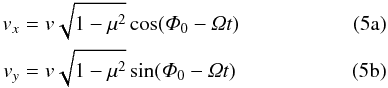denote the unperturbed, quasi-linear, orbits with Ω the gyrofrequency and Φ₀ the initial gyro phase.

Squaring and taking the ensemble average yields $\begin{array}{ccc}\mathrm{⟨}{\left(\mathit{\Delta \mu }\mathrm{\left(}\mathit{t}\mathrm{\right)}\right)}^{\mathrm{2}}\mathrm{⟩}& \mathrm{=}& \frac{{\mathit{\Omega }}^{\mathrm{2}}\mathrm{(}\mathrm{1}\mathrm{-}{\mathit{\mu }}^{\mathrm{2}}\mathrm{)}}{{\mathit{B}}_{\mathrm{0}}^{\mathrm{2}}}{\mathrm{\int }}_{\mathrm{0}}^{\mathit{t}}\mathrm{d}{\mathit{t}}^{\mathrm{\prime }}{\mathrm{\int }}_{\mathrm{0}}^{\mathit{t}}\mathrm{d}{\mathit{t}}^{\mathrm{\prime \prime }}\\ & & \mathrm{\times }\cos \left[\mathit{\Omega }\left({\mathit{t}}^{\mathrm{\prime }}\mathrm{-}{\mathit{t}}^{\mathrm{\prime \prime }}\right)\right]⟨\mathit{\delta }{\mathit{B}}_{\mathit{x}}\mathrm{\left(}{\mathit{t}}^{\mathrm{\prime }}\mathrm{\right)}\hspace{0.17em}\mathit{\delta }{\mathit{B}}_{\mathit{x}}\mathrm{\left(}{\mathit{t}}^{\mathrm{\prime \prime }}\mathrm{\right)}⟩\mathit{.}\end{array}$(6)After taking the Fourier transform, the magnetic correlation tensor element P_xx(k) can be inserted.

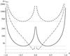Fig. 2 Critical time, tmax, as obtained from the numerical solution of Eq. (7)for particles with different pitch angles. The solid and dot-dashed lines show the cases of particles with rigidity values chosen as R = 1 and R = 10, respectively, with a relative turbulence strength of δB/B0 = 10-1. For the dashed line, parameters are R = 1 and δB/B0 = 10-1.5. The dotted lines show the minimum of the critical time for all pitch angles.

For instance, by assuming slab geometry and setting τ = Ωt, the result can finally be expressed as (cf. Shalchi 2005) $\mathrm{⟨}{\left(\mathit{\Delta \mu }\mathrm{\left(}\mathit{\tau }\mathrm{\right)}\right)}^{\mathrm{2}}\mathrm{⟩}\mathrm{=}\mathrm{4}\mathit{\pi }\mathrm{(}\mathrm{1}\mathrm{-}{\mathit{\mu }}^{\mathrm{2}}\mathrm{)}{\left(\frac{\mathit{\delta B}}{{\mathit{B}}_{\mathrm{0}}}\right)}^{\mathrm{2}}{\mathrm{\int }}_{\mathrm{0}}^{\mathrm{\infty }}\mathrm{d}\mathit{kG}\mathrm{\left(}\mathit{k}\mathrm{\right)}\left[{\mathrm{𝒦}}_{\mathrm{+}}\mathrm{+}{\mathrm{𝒦}}_{\mathrm{-}}\right]\mathit{,}$(7)where the spectrum G(k) from Eq. (A.2)has been used. In what follows, normalized variables are used as R = γv/(Ωℓ₀), and x = ℓ₀k; the resonance functions can then be expressed as ${\mathrm{𝒦}}_{\mathrm{\pm }}\mathrm{=}\frac{\mathrm{1}\mathrm{-}\cos \left[\left(\mathit{xR\mu }\mathrm{\pm }\mathrm{1}\right)\mathit{\tau }\right]}{{\left(\mathit{xR\mu }\mathrm{\pm }\mathrm{1}\right)}^{\mathrm{2}}}\mathrm{·}$(8)By requiring that , the critical time t_max can be obtained by (numerically) solving Eq. (7)for the time. The result is shown in Fig. 2 and confirms the estimation that, for stronger turbulence, the increased scattering causes particles to reach the limiting pitch angle values earlier.

For other turbulence geometries – especially isotropic turbulence – the same analysis is possible in principle, although the required calculations become somewhat unwieldy (cf. Tautz et al. 2008; Tautz & Lerche 2010).

3.3. Pitch-angle distribution

In this paragraph, it is demonstrated that particles stay in their original pitch-angle regime for all times. This is true even if, as stated above, the Fokker-Planck coefficient of pitch-angle scattering tends to zero for times t > t_max.

In Fig. 3, the distribution function of all particles sorted for their pitch-angle displacement, Δμ, is shown. As time increases, particles begin to deviate from their original pitch angles. Nevertheless (note the logarithmic scaling of the vertical axis!), the distribution remains extremely small with its width growing linearly with time as 10^-5Ωt.

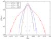Fig. 3 Distribution function f(Δμ) of the relative pitch-angle displacement, Δμ = μ(t) − μ0, for three different times. The horizontal dotted bars show the corresponding standard deviations. Additionally, the vertical dotted line shows the mean (which remains almost unchanged). (This figure is available in color in electronic form)

In Fig. 4, the time evolution of a Kolmogorov-Smirnov (KS) test statistic is shown, which is obtained from the comparison of the pitch-angle distribution, f(μ,t), with the initial pitch-angle distribution, f(μ₀,0). Because the latter is obtained from a uniform random deviate, the usual result of an isotropized distribution due to pitch-angle diffusion leads to the requirement that the pitch-angle distribution be uniform. A linear fit of the otherwise relatively volatile KS statistic shows that, on average, the P value (i.e., the probability that the given distribution agrees with the assumed one) of the KS test is well above 80%; this confirms that the pitch-angle distribution remains compatible with the initial distribution.

This result serves as a second indicator that an initially homogeneous pitch-angle distribution is retained. As a side note, it should be mentioned that the pitch-angle distribution is not precisely homogeneous, i.e., the comparison of the pitch-angle distribution with a flat distribution yields a reduced KS test statistic as opposed to the comparison of f(μ,t) with f(μ₀).

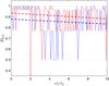Fig. 4 Time evolution of the KS test statistic (solid lines) for the agreement between the pitch-angle distribution, f(μ,t), and the initial distribution, f(μ0,0) (which are obtained from uniform random deviates) together with linear fits (dashed lines). The red and blue lines correspond to the cases of low and intermediate turbulence strength, respectively. (This figure is available in color in electronic form)

4. Fokker-Planck coefficient

In this section, some of the intricacies connected to the numerical implementation of pitch-angle scattering is discussed. For an overview of analytical calculations, the reader is referred to Appendix A, where both quasi-linear and nonlinear results are summarized.

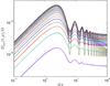Fig. 5 Running pitch-angle Fokker-Planck coefficient, Dμμ(t), for various values of the initial pitch-angle cosine, μ0, which is represented by the different colors. For the numerical evaluation, Eq. (3)has been used, together with the procedure described thereafter. Other parameters are identical to those in Fig. 1. (This figure is available in color in electronic form)

While the calculation of the mean free path values is straightforward, this is somewhat different for the Fokker-Planck coefficient(s). Especially D_μμ has to be a function of time but, at the same time, depends on the μ values. It has to be stressed that pitch-angle scattering is unique in that, unlike for normal spatial diffusion, the coefficient depends on the variable from which the mean square displacement is obtained.

Therefore, several options are possible, two of which will be described here.

• Particles are binned once and for all to μ slots according to their initial pitch-angle, μ(0) ≡ μ₀. While at first glance this procedure seems to be justified by the fact that Eq. (3)is symmetric in μ(t) and μ₀, it has the crucial drawback of conserving the initial conditions. However, a diffusive process is defined as a process that has become independent of the initial condition; therefore, this approach has to be discarded.

• In an alternative approach, as opposed to the one described above, particles are binned separately at each point in time to μ slots. Average values are then taken for all particles in a given μ slot, thereby obtaining D_μμ(μ,t) as a function of pitch angle and time. In principle, both Eqs. (2b)and (3)should be interchangeable. In practice, however, it turns out that the derivative is considerably more volatile, while Eq. (3)yields reasonable results even for a moderate number of particles.

The second approach is illustrated in Fig. 5 for various pitch angles. By evaluating Eq. (3), a Fokker-Planck coefficient is obtained that depends both on the time and on the pitch-angle cosine. Plotted as a function of time, the transition to the diffusive regime can be seen for times t ≃ 5Ω^-1. For times , it is admissible to take asymptotic values for the Fokker-Planck coefficient as a function of the pitch-angle cosine, i.e., D_μμ(μ).

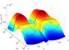Fig. 6 Running Fokker-Planck coefficient of pitch-angle scattering, Dμμ(μ,t) for particles width rigidity R = 10-2 in moderate turbulence strength, δB/B0 = 10-1.5. The black solid lines illustrate Dμμ(μ) at specific times. (This figure is available in color in electronic form)

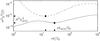Fig. 7 Time evolution of the χ2 value associated with the running Fokker-Planck coefficient of pitch-angle scattering as shown in Fig. 6. The solid and dashed lines show the cases of R = 10-2 and R = 10-1, respectively, with δB/B0 = 10-1.5 for both cases. The χ2 value is obtained from the comparison with Eq. (A.3).

In Fig. 6, the time evolution of the pitch-angle Fokker-Planck coefficient is illustrated. The typical double-hump structure known from analytical theories (cf. Appendix A) is exhibited; for later times, in contrast, the characteristic 1/t dependence shown in Eq. (2b)dominates. Additionally, the shape of D_μμ is strongly modified, thereby resulting in a drastically increased χ² for the comparison between simulation and analytical theory as shown in Fig. 7.

5. Comparison with analytical results

In this section, the numerical results for the Fokker-Planck coefficient will be compared to analytical results listed in Appendix A. Error bars are obtained from the comparison of different turbulence realizations and different initial particle positions (see Tautz 2010). In addition, it has to be stressed again that, according to Fig. 6, the correct time point has to be chosen for the evaluation of D_μμ.

5.1. Slab turbulence

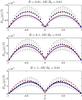Fig. 8 Numerically calculated pitch-angle Fokker-Planck coefficient, Dμμ, as a function of the pitch-angle cosine, μ, for three different values for the normalized rigidity, R. For comparison, the analytical results from QLT and SOQLT are shown as solid blue and dashed red lines, respectively. The relative turbulence strength is chosen as δB/B0 = 10-2. (This figure is available in color in electronic form)

In Fig. 5, the pitch-angle Fokker-Planck coefficient is shown as a function of the normalized simulation time, τ = Ωt. After the initial free-streaming phase, most values become (almost) constant, while the initially higher values still oscillate. At τ = 10², the final, diffusive values for D_μμ are taken that are used in the following sections. It should be noted, however, that D_μμ is slightly decreasing (with approximately  ∝ τ^-0.14) so that the values for D_μμ are somewhat overestimated, in agreement with the results shown below.

In the following, the two cases of low and intermediate turbulence strengths are discussed.

5.1.1. Low turbulence strength

For the ratio of the turbulent and background magnetic fields, a value of δB/B₀ = 10^-2 is chosen so that the ratio of the magnetic field energies is (δB/B₀)² = 10^-4. The following results were found (see Fig. 8):

• For small and intermediate rigidities ranging fromR = 10^-2 to 10^-1, an excellent agreement between numerical and analytical results can be found. However, QLT and SOQLT are almost indistinguishable. For example, a chi-square test yields values of χ² = 6.551 and 6.432 at R = 10^-1 for the comparison to QLT and SOQLT, respectively, thereby revealing that the agreement with SOQLT is slightly better. However, the difference is marginal and might have occurred purely by serendipity.

• For high rigidities such as R = 1 and R = 10, QLT and SOQLT differ more. A chi-square test yields values of χ² = 2.531 and 28.81 at R = 1 for the comparison to QLT and SOQLT, respectively, thereby revealing that the agreement with QLT is significantly better. However, it should be noted that the approximation used for the SOQLT values becomes invalid if R is too large.

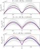Fig. 9 Same as Fig. 8, only that now the relative turbulence strength is chosen as δB/B0 = 10-1.5 ≈ 0.0316. (This figure is available in color in electronic form)

5.1.2. Intermediate turbulence strength

Here, δB/B₀ = 10^-1.5 ≈ 0.0316 is chosen so that the ratio of the magnetic field energies is 10^-3. The following results were found (see Fig. 9):

• For small and intermediate rigidities, the simulation results agreeequally well with both QLT and SOQLT, to the same level ofsignificance as was found in the previous section.

• For high rigidities, it is shown that both QLT and SOQLT severely underestimate 90° scattering, even though SOQLT was designed explicitly to remedy this shortcoming of previous, quasi-linear results. Accordingly, the chi-square test yields slightly higher values of χ² = 13.55 and 14.05 at R = 1 for QLT and SOQLT, respectively, which again shows that QLT agrees slightly better with the numerical values.

• Additionally, it is remarkable that, for R = 10, the overall best agreement has been found as expressed by the low value χ² = 2.24.

In general, it has to be noted (cf. Table 1) that the agreement between analytical and numerical results depends on the maximum simulation time. For t ≠ t_max, less agreement is found.

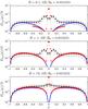Fig. 10 Same as Fig. 9, only that now the case of isotropic turbulence is shown. Due to the complexity of the SOQLT, the evaluation is given at some discrete points instead of as a continuous function. (This figure is available in color in electronic form)

5.2. Isotropic turbulence

For isotropic turbulence, the numerical Fokker-Planck coefficient is shown in Fig. 10. The comparison especially with SOQLT had to be done for higher rigidities than for slab geometry simply because the numerical evaluation of Eq. (A.5)is extremely protracted for low rigidities and/or low turbulence strengths.

While the agreement between theory and simulation is generally good at pitch-angles well off 90°, it is revealed that 90° degree scattering is not equally well described either by QLT or by SOQLT. Therefore, the agreement of the parallel mean free path with simulations (cf. Tautz et al. 2008; Tautz & Lerche 2010) has to be attributed to the fact that, at μ = 0, SOQLT overestimates D_μμ, thereby compensating for values that are too low at .

6. Summary and conclusion

In this paper, random variations in the pitch-angle of charged particles that move in a turbulent magnetic field have been investigated. In the astrophysical theater, this situation is realized by cosmic rays and solar particle events, both of which experience continuous deflections either in the interstellar turbulence or in the solar-wind induced turbulence. In both cases, the random component superposes a mean magnetic field – e.g., the galactic magnetic field or the Parker-spiral solar magnetic field – which gives rise to a preferred direction when investigating the scattering processes. This motivates the transformation to a coordinate system in which the pitch angle is taken to be a basic variable of the particle motion.

The process can be analyzed by means of analytic calculations and numerical Monte-Carlo simulations, which are methods based on the kinetic Vlasov theory and the integration of the equation of motion for a large number of test particles, respectively. Whereas the use of a Fokker-Planck approach to determining the pitch-angle scattering and, based thereupon, the parallel mean-free path, has been established decades ago, it has been difficult to reproduce the process using test-particle simulations. The reason is not only that, owing to the required pitch-angle resolution of the Fokker-Planck coefficient, a large number of particles are required, but that, additionally, the underlying algorithm is not entirely clear. While there are previous simulations (Qin & Shalchi 2009) that confirm quasi-linear results, here we have shown that the time dependence of the Fokker-Planck coefficient cannot be neglected.

Instead, one general result that has been found is the following: because the pitch-angle cosine, μ, is confined to μ ∈  [−1,1] , pitch-angle scattering as based on Eqs (2b)and (3)is not a process that can be described for asymptotically long times. Instead, the proper time has to be found where (i) D_μμ is no longer dominated by the initial conditions; but (ii) D_μμ is not yet dominated by the 1/t dependence because Δμ cannot grow any further. However, with the additional constraint that the turbulence strength is not too high, there always seems to be a time period where excellent agreement with the analytical results can be obtained.

The important question that has to be raised, therefore, is the validity of the generally accepted formulae for the Fokker-Planck coefficient. In order to account for the deviations found in the present paper, in a second paper the underlying theoretical basis of the pitch-angle Fokker-Planck coefficient as based on the diffusion equation will be revisited.

Acknowledgments

R.C.T. thanks Gary Zank, Fathallah Alouani-Bibi, and Andreas Shalchi for useful discussions on the subject of pitch-angle scattering.

References

Appendix A: Analytical pitch-angle scattering

Analytically, the Fokker-Planck coefficient of pitch-angle scattering can be evaluated, e.g., using quasilinear theory (Jokipii 1966) and nonlinear extensions (see Shalchi 2009, for an overview). In any case, the evaluation is based on the TGK formalism by using Eq. (2a).

A.1. Slab turbulence

For slab turbulence, the result is (e.g., Qin & Shalchi 2009) 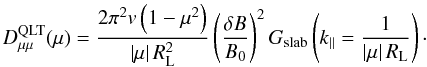${\mathit{D}}_{\mathit{\mu \mu }}^{\mathrm{QLT}}\mathrm{\left(}\mathit{\mu }\mathrm{\right)}\mathrm{=}\frac{\mathrm{2}{\mathit{\pi }}^{\mathrm{2}}\mathit{v}\mathrm{(}\mathrm{1}\mathrm{-}{\mathit{\mu }}^{\mathrm{2}}\mathrm{)}}{\left|\mathit{\mu }\right|{\mathit{R}}_{\mathrm{L}}^{\mathrm{2}}}{\left(\frac{\mathit{\delta B}}{{\mathit{B}}_{\mathrm{0}}}\right)}^{\mathrm{2}}{\mathit{G}}_{\mathrm{slab}}\left({\mathit{k}}_{\mathrm{\parallel }}\mathrm{=}\frac{\mathrm{1}}{\left|\mathit{\mu }\right|{\mathit{R}}_{\mathrm{L}}}\right)\mathrm{·}$(A.1)For the turbulence power spectrum, G(k), a kappa-type function is used (Shalchi & Weinhorst 2009): $\mathit{G}\mathrm{\left(}\mathit{k}\mathrm{\right)}\mathrm{=}\frac{\mathit{C}}{\mathrm{2}\sqrt{\mathit{\pi }}}\hspace{0.17em}\frac{\mathit{\Gamma }\mathrm{(}\mathit{s}\mathit{/}\mathrm{2}\mathrm{)}}{\mathit{\Gamma }(\mathrm{(}\mathit{s}\mathrm{-}\mathrm{1}\mathrm{)}\mathit{/}\mathrm{2})}\frac{{\left|{\mathit{\ell }}_{\mathrm{0}}\mathit{k}\right|}^{\mathit{q}}}{{\mathrm{[}\mathrm{1}\mathrm{+}{\mathrm{(}{\mathit{\ell }}_{\mathrm{0}}{\mathit{k}}^{\mathrm{)}}}^{\mathrm{2}}\mathrm{]}}^{\mathit{s}\mathit{/}\mathrm{2}}}\mathit{,}$(A.2)with usually q = 0 for simplicity. The turbulence bend-over scale, ℓ₀ ≈ 0.03 AU, reflects the transition from the energy range G(k) ∝ k^q to the Kolmogorov-type inertial range, where G(k) ∝ k^−s with s = 5/3 for large wavenumbers (Kolmogorov 1991; Bruno & Carbone 2005). The factor C depends on the assumed geometry and is given as C = 1/(2π) for slab turbulence, where δB(r) = δB(z), and C = 4 for isotropic turbulence.

In the normalized variables R and τ, the Fokker-Planck coefficient of pitch-angle scattering can be expressed as 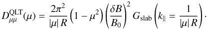${\mathit{D}}_{\mathit{\mu \mu }}^{\mathrm{QLT}}\mathrm{\left(}\mathit{\mu }\mathrm{\right)}\mathrm{=}\frac{\mathrm{2}{\mathit{\pi }}^{\mathrm{2}}}{\left|\mathit{\mu }\right|\mathit{R}}\mathrm{(}\mathrm{1}\mathrm{-}{\mathit{\mu }}^{\mathrm{2}}\mathrm{)}{\left(\frac{\mathit{\delta B}}{{\mathit{B}}_{\mathrm{0}}}\right)}^{\mathrm{2}}{\mathit{G}}_{\mathrm{slab}}\left({\mathit{k}}_{\mathrm{\parallel }}\mathrm{=}\frac{\mathrm{1}}{\left|\mathit{\mu }\right|\mathit{R}}\right)\mathrm{·}$(A.3)The typical (1 − μ²) dependence reflects the fact that particles with pitch angles close to 0° and 180° are considerably less scattered than particles with intermediate pitch angles; in addition, the rightmost factor in Eq. (A.3)approximately gives |μ|^2/3, thereby suppressing 90° scattering.

A nonlinear theory developed especially to enhance pitch-angle scattering through 90° (Shalchi 2005, 2009) yields the formula $\begin{array}{ccc}{\mathit{D}}_{\mathit{\mu \mu }}& \mathrm{=}& \frac{\mathrm{1}}{\mathrm{8}\mathit{s}\sqrt{\mathit{\pi }}}\hspace{0.17em}\frac{\mathit{\Gamma }\mathrm{(}\mathit{s}\mathit{/}\mathrm{2}\mathrm{)}}{\mathit{\Gamma }(\mathrm{(}\mathit{s}\mathrm{-}\mathrm{1}\mathrm{)}\mathit{/}\mathrm{2})}\mathrm{(}\mathrm{1}\mathrm{-}{\mathit{\mu }}^{\mathrm{2}}\mathrm{)}\mathit{C}\mathrm{\left(}\mathit{s}\mathrm{\right)}\hspace{0.17em}\frac{{\mathit{R}}^{\mathrm{2}\mathrm{-}\mathit{s}}\mathit{v}}{{\mathit{\ell }}_{\mathrm{0}}}\hspace{0.17em}\frac{\mathit{\delta B}}{{\mathit{B}}_{\mathrm{0}}}\\ & & \mathrm{\times }\sum _{\mathit{n}\mathrm{=}\mathrm{\pm }\mathrm{1}}\mathrm{sgn}\left(\frac{\mathit{\delta B}}{{\mathit{B}}_{\mathrm{0}}}\mathrm{+}\mathit{n}\left|\mathit{\mu }\right|\right){\left|\left|\mathit{\mu }\right|\mathrm{+}\mathit{n}\hspace{0.17em}\frac{\mathit{\delta B}}{{\mathit{B}}_{\mathrm{0}}}\right|}^{\mathit{s}}\end{array}$(A.4)where R and v are the normalized rigidity and the particle speed, respectively.

A.2. Isotropic turbulence

For isotropic turbulence, the analytical theory of pitch-angle scattering is considerably more difficult to solve (Tautz et al. 2006, 2008). The general form of the Fokker-Planck coefficient for pitch-angle scattering¹ reads as $\begin{array}{ccc}{\mathit{D}}_{\mathit{\mu \mu }}& \mathrm{=}& \mathrm{2}\mathrm{(}\mathrm{1}\mathrm{-}{\mathit{\mu }}^{\mathrm{2}}\mathrm{)}{\mathit{\Omega }}^{\mathrm{2}}{\left(\frac{\mathit{\delta B}}{{\mathit{B}}_{\mathrm{0}}}\right)}^{\mathrm{2}}{\mathrm{\int }}_{\mathrm{0}}^{\mathrm{1}}\mathrm{d}\mathit{\eta }{\mathrm{\int }}_{\mathrm{0}}^{\mathrm{\infty }}\mathrm{d}\mathit{kG}\mathrm{\left(}\mathit{k}\mathrm{\right)}\\ & & \end{array}$(A.5)with J_n(w) the Bessel function of the first kind of order n and $\mathit{w}\mathrm{=}\mathrm{(}\mathit{kv}\mathit{/}\mathit{\Omega }\mathrm{)}\sqrt{\mathrm{(}\mathrm{1}\mathrm{-}{\mathit{\mu }}^{\mathrm{2}}\mathrm{)}\mathrm{(}\mathrm{1}\mathrm{-}{\mathit{\eta }}^{\mathrm{2}}\mathrm{)}}$. Additionally, η = cos∠(k,B₀) is the wave vector polar angle. The resonance function can be expressed as ${\mathrm{ℛ}}_{\mathit{n}}\mathrm{\left(}\mathit{k,\eta }\mathrm{\right)}\mathrm{=}\mathit{\pi \delta }\left(\mathit{kv\mu \eta }\mathrm{+}\mathit{n\Omega }\right)$(A.6a)for QLT and ${\mathrm{ℛ}}_{\mathit{n}}\mathrm{\left(}\mathit{k,\eta }\mathrm{\right)}\mathrm{=}\sqrt{\frac{\mathit{\pi }}{\mathrm{2}}}{\left(\mathit{\xi k\eta }\right)}^{-1}\exp \left[\mathrm{-}\frac{{\left(\mathit{kv\mu \eta }\mathrm{+}\mathit{n\Omega }\right)}^{\mathrm{2}}}{\mathrm{2}{\left(\mathit{k\eta \xi }\right)}^{\mathrm{2}}}\right]$(A.6b)for SOQLT, where ξ = v²(δB/B₀)²/3. Using QLT, Eq. (A.5)can be simplified further (see Tautz et al. 2006), whereas, for SOQLT, the two integrals and the infinite sum have to be evaluated numerically.

Alternatively, the formulation of Tautz & Lerche (2010) can be used for the case of SOQLT, where the infinite sum over Bessel functions was reduced to a closed form analytical expression under the assumption of a Cauchy-type resonance function.

All Tables

All Figures

	Fig. 1 Pitch-angle cosine, μ = v ∥ /v as a function of the normalized time, τ = Ωt for a relative slab turbulence strength δB/B0 = 10-2. Four particles with initial pitch angles in the range 0.1 ≲ μ0 ≲ 0.8 are highlighted to guide the eye. (This figure is available in color in electronic form)
In the text

Fig. 2 Critical time, tmax, as obtained from the numerical solution of Eq. (7)for particles with different pitch angles. The solid and dot-dashed lines show the cases of particles with rigidity values chosen as R = 1 and R = 10, respectively, with a relative turbulence strength of δB/B0 = 10-1. For the dashed line, parameters are R = 1 and δB/B0 = 10-1.5. The dotted lines show the minimum of the critical time for all pitch angles.

In the text

	Fig. 3 Distribution function f(Δμ) of the relative pitch-angle displacement, Δμ = μ(t) − μ0, for three different times. The horizontal dotted bars show the corresponding standard deviations. Additionally, the vertical dotted line shows the mean (which remains almost unchanged). (This figure is available in color in electronic form)
In the text

Fig. 4 Time evolution of the KS test statistic (solid lines) for the agreement between the pitch-angle distribution, f(μ,t), and the initial distribution, f(μ0,0) (which are obtained from uniform random deviates) together with linear fits (dashed lines). The red and blue lines correspond to the cases of low and intermediate turbulence strength, respectively. (This figure is available in color in electronic form)

In the text

	Fig. 5 Running pitch-angle Fokker-Planck coefficient, Dμμ(t), for various values of the initial pitch-angle cosine, μ0, which is represented by the different colors. For the numerical evaluation, Eq. (3)has been used, together with the procedure described thereafter. Other parameters are identical to those in Fig. 1. (This figure is available in color in electronic form)
In the text

	Fig. 6 Running Fokker-Planck coefficient of pitch-angle scattering, Dμμ(μ,t) for particles width rigidity R = 10-2 in moderate turbulence strength, δB/B0 = 10-1.5. The black solid lines illustrate Dμμ(μ) at specific times. (This figure is available in color in electronic form)
In the text

	Fig. 7 Time evolution of the χ2 value associated with the running Fokker-Planck coefficient of pitch-angle scattering as shown in Fig. 6. The solid and dashed lines show the cases of R = 10-2 and R = 10-1, respectively, with δB/B0 = 10-1.5 for both cases. The χ2 value is obtained from the comparison with Eq. (A.3).
In the text

Fig. 8 Numerically calculated pitch-angle Fokker-Planck coefficient, Dμμ, as a function of the pitch-angle cosine, μ, for three different values for the normalized rigidity, R. For comparison, the analytical results from QLT and SOQLT are shown as solid blue and dashed red lines, respectively. The relative turbulence strength is chosen as δB/B0 = 10-2. (This figure is available in color in electronic form)

In the text

	Fig. 9 Same as Fig. 8, only that now the relative turbulence strength is chosen as δB/B0 = 10-1.5 ≈ 0.0316. (This figure is available in color in electronic form)
In the text

	Fig. 10 Same as Fig. 9, only that now the case of isotropic turbulence is shown. Due to the complexity of the SOQLT, the evaluation is given at some discrete points instead of as a continuous function. (This figure is available in color in electronic form)
In the text

References

- Belcher, J. W., & Davis, L. 1971, J. Geophys. Res., 76, 3534 [NASA ADS] [CrossRef] [Google Scholar]
- Beresnyak, A., Yan, H., & Lazarian, A. 2011, ApJ, 728, 60 [NASA ADS] [CrossRef] [Google Scholar]
- Bieber, J. W., Smith, C. W., & Matthaeus, W. H. 1988, ApJ, 334, 470 [NASA ADS] [CrossRef] [Google Scholar]
- Bieber, J. W., Wanner, W., & Matthaeus, W. H. 1996, J. Geophys. Res., 101, 2511 [Google Scholar]
- Bruno, R., & Carbone, V. 2005, Liv. Rev. Sol. Phys., 2, 1 [Google Scholar]
- Chandrasekhar, S. 1943, Rev. Mod. Phys., 15, 1 [NASA ADS] [CrossRef] [Google Scholar]
- Decker, R. B., Krimigis, S. M., Roelof, E. C., et al. 2005, Science, 309, 2020 [NASA ADS] [CrossRef] [PubMed] [Google Scholar]
- Dröge, W. 2000, Space Sci. Rev., 93, 121 [NASA ADS] [CrossRef] [Google Scholar]
- Dunzlaff, P., Kopp, A., & Heber, B. 2010, J. Geophys. Res. (Space Phys.), 115, 10106 [NASA ADS] [CrossRef] [Google Scholar]
- Ferrando, P., Ducros, R., Rastoin, C., & Raviart, A. 1993, Planet. Space Sci., 41, 839 [NASA ADS] [CrossRef] [Google Scholar]
- Fick, A. 1855, Ann. Phys., 170, 59 [NASA ADS] [CrossRef] [Google Scholar]
- Fisk, L. A., Goldstein, M. L., Klimas, A. J., & Sandri, G. 1974, ApJ, 190, 417 [NASA ADS] [CrossRef] [Google Scholar]
- Florinski, V., Decker, R. B., & Le Roux, J. A. 2008, J. Geophys. Res. (Space Phys.), 113, 7103 [NASA ADS] [CrossRef] [Google Scholar]
- Goldreich, P., & Sridhar, S. 1995, ApJ, 438, 763 [NASA ADS] [CrossRef] [Google Scholar]
- Green, M. S. 1951, J. Chem. Phys., 19, 1036 [Google Scholar]
- Jokipii, J. R. 1966, ApJ, 146, 480 [Google Scholar]
- Kelly, J., Dalla, S., & Laitinen, T. 2012, ApJ, 750, 47 [NASA ADS] [CrossRef] [Google Scholar]
- Kolmogorov, A. N. 1991, Proc. Royal Soc. London, Ser. A: Math. Phys. Sci., 434, 9 [Google Scholar]
- Kubo, R. 1957, J. Phys. Soc. Japan, 12, 570 [Google Scholar]
- Laitinen, T., Dalla, S., & Kelly, J. 2012, ApJ, 749, 103 [NASA ADS] [CrossRef] [Google Scholar]
- Laitinen, T., Dalla, S., Kelly, J., & Marsh, M. 2013, ApJ, 764, 168 [Google Scholar]
- Lemons, D. S., Liu, K.-J., Winske, D., & Gary, S. P. 2009, Phys. Plasmas, 16, 112306 [NASA ADS] [CrossRef] [Google Scholar]
- le Roux, J. A., & Webb, G. M. 2012, ApJ, 746, 104 [NASA ADS] [CrossRef] [Google Scholar]
- Matthaeus, W. H., Goldstein, M. L., & Roberts, D. A. 1990, J. Geophys. Res., 95, 20673 [Google Scholar]
- Qin, G., & Shalchi, A. 2009, ApJ, 707, 61 [NASA ADS] [CrossRef] [Google Scholar]
- Rausch, M., & Tautz, R. C. 2013, MNRAS, 428, 2333 [NASA ADS] [CrossRef] [Google Scholar]
- Roelof, E. C. 1969, in Lectures in High-Energy Astrophysics, eds. H. Ögelman, & J. R. Wayland, 111 [Google Scholar]
- Schlickeiser, R. 1989, ApJ, 336, 243 [NASA ADS] [CrossRef] [Google Scholar]
- Schlickeiser, R. 2002, Cosmic Ray Astrophysics (Berlin: Springer) [Google Scholar]
- Shalchi, A. 2005, Phys. Plasmas, 12, 052905 [Google Scholar]
- Shalchi, A. 2009, Nonlinear Cosmic Ray Diffusion Theories (Berlin: Springer) [Google Scholar]
- Shalchi, A. 2011, Phys. Rev. E, 83, 046402 [NASA ADS] [CrossRef] [Google Scholar]
- Shalchi, A., & Weinhorst, B. 2009, Adv. Space Res., 43, 1429 [NASA ADS] [CrossRef] [Google Scholar]
- Shalchi, A., Škoda, T., Tautz, R. C., & Schlickeiser, R. 2009, Phys. Rev. D, 80, 023012 [Google Scholar]
- Spanier, F., & Wisniewski, M. 2011, Astrophys. Space Sci. Transact., 7, 21 [NASA ADS] [CrossRef] [Google Scholar]
- Sridhar, S., & Goldreich, P. 1994, ApJ, 432, 612 [NASA ADS] [CrossRef] [Google Scholar]
- Tautz, R. C. 2010, Comp. Phys. Commun., 81, 71 [NASA ADS] [CrossRef] [Google Scholar]
- Tautz, R. C. 2012, in Turbulence: Theory, Types and Simulation, ed. R. J. Marcuso (New York: Nova Publishers), 365 [Google Scholar]
- Tautz, R. C. 2013, A&A, 558, A148 [NASA ADS] [CrossRef] [EDP Sciences] [Google Scholar]
- Tautz, R. C., & Dosch, A. 2013, Phys. Plasmas, 20, 022302 [NASA ADS] [CrossRef] [Google Scholar]
- Tautz, R. C., & Lerche, I. 2010, Phys. Lett. A, 374, 4573 [NASA ADS] [CrossRef] [Google Scholar]
- Tautz, R. C., & Shalchi, A. 2013, J. Geophys. Res., 118, 642 [Google Scholar]
- Tautz, R. C., Shalchi, A., & Schlickeiser, R. 2006, J. Phys. G: Nuclear Part. Phys., 32, 809 [NASA ADS] [CrossRef] [Google Scholar]
- Tautz, R. C., Shalchi, A., & Schlickeiser, R. 2008, ApJ, 685, L165 [NASA ADS] [CrossRef] [Google Scholar]
- Tautz, R. C., Shalchi, A., & Dosch, A. 2011, J. Geophys. Res. (Space Phys.), 116, 2102 [Google Scholar]
- Taylor, G. I. 1922, Proc. London Math. Soc., 20, 196 [Google Scholar]
- Wisniewski, M., Spanier, F., & Kissmann, R. 2012, ApJ, 750, 150 [NASA ADS] [CrossRef] [Google Scholar]