| Issue |
A&A
Volume 558, October 2013
|
|
|---|---|---|
| Article Number | A115 | |
| Number of page(s) | 7 | |
| Section | Astrophysical processes | |
| DOI | https://doi.org/10.1051/0004-6361/201321876 | |
| Published online | 15 October 2013 | |
Conical fireballs, cannonballs, and jet breaks in the afterglows of gamma ray bursts
Physics Department,
Technion,
32000
Haifa,
Israel
Received:
10
May
2013
Accepted:
17
August
2013
Abstract
The jet break in the X-ray afterglow of gamma ray bursts (GRBs) appears to be correlated to other properties of the X-ray afterglow and the prompt gamma ray emission, but the correlations are at odds with those predicted by the conical fireball (FB) model of GRBs. They are in good agreement, however, with those predicted by the cannonball (CB) model of GRBs.
Key words: gamma-ray burst: general
© ESO, 2013
1. Introduction
Before the launch of the Compton Gamma Ray Observatory (CGRO) in 1991 it was widely believed that gamma-ray bursts (GRBs) originate in the Galaxy or in its halo. Much larger distances together with the observed fast rise time of GRB pulses implied an energy crisis – implausible energy release in gamma rays from a very small volume in a short time, if the emission was isotropic, as was generally assumed. However, the isotropic distribution of GRBs over the sky and their intensity distribution that were measured with the Burst and Transient Source Experiment (BATSE) aboard CGRO shortly after its launch provided clear evidence that the observed GRBs are at very large cosmological distances (Meegan et al. 1992; Mao & Paczynski 1992). That led Shaviv & Dar (1995) to propose that GRBs are produced by inverse Compton scattering of light by highly relativistic jets whose radiation is narrowly beamed along their direction of motion and that such jets are presumably ejected following violent stellar processes such as core collapse supernovae, merger of compact stars, mass accretion on compact stars and phase transition in compact stars, rather than in spherical fireballs (FBs; Paczynski 1986; Goodman 1986) produced by neutron star merger in close binaries (Goodman et al. 1987). These jets were assumed to be a succession of highly relativistic plasmoids of ordinary matter like those observed in high-resolution observations of highly relativistic jets ejected from galaxies with active galactic nucleus (e.g., M87 in Virgo), from radio galaxies (e.g., Centaurus A, the nearest radio galaxy), from quasars (e.g., 3C 273 in Virgo), and from microquasars (e.g., GRS 1915+105, SS 433, Cygnus X-1, and Cygnus X-3 in our Galaxy). A key prediction of such a model was a very high linear polarization (P ~ 100%) of gamma rays observed from the most probable viewing angle of the GRBs (Shaviv & Dar 1995).
The hypothesis that GRBs are produced by highly relativistic jets was not widely accepted even when the discovery of the X-ray afterglows of GRBs by the Beppo-SAX satellite (Costa et al. 1997) allowed their arcminute localization, which led to the discovery of their longer wavelength afterglows (van Paradijs et al. 1997; Frail et al. 1997), host galaxies (Sahu et al. 1997), and their high redshifts (Metzger et al. 1997). In fact, the discovery of GRB afterglows, which appeared to decay like a single powerlaw in time, as predicted by Paczynski & Rhoads (1993), Katz (1994) and Mezaros & Rees (1997) from the isotropic FB model (Paczynski 1986; Goodman 1986), led to an immediate, wide acceptance of the relativistic isotropic FB model as the correct description of GRBs and their afterglows (see, e.g., Wijers et al. 1997; Piran 1999), ignoring the energy crisis of the isotropic FB model of GRBs.
When data on redshifts and afterglows of GRBs began to accumulate, it became clear that GRBs could not be explained by the isotropic FB model (e.g., Dar 1998). Not only did their high redshifts imply implausible energy release in gamma rays if the emission was isotropic, but their observed afterglows also seemed to behave like a smoothly broken powerlaw in time (Beuermann et al. 1999; Fruchter et al. 1999; Harrison et al. 1999; Kulkarni et al. 1999) rather than like a single power law. Only then was the isotropic FB replaced (e.g., Sari et al. 1999; Piran 1999, 2000) by an assumed conical jet of thin shells where synchrotron radiation from collisions between overtaking shells (or internal shocks) produce the observed GRB pulses, and the following collision of the merged shells with the interstellar medium (ISM) produces the synchrotron afterglow. This conical jet model which was given the name collimated FB model, replaced the original FB model, but retained its name the FB model.
The afterglow of a conical shell of opening angle θj, whose propagation is decelerated by sweeping up the ISM in front of it, was shown by Sari et al. (1999) to have an achromatic break when its bulk motion Lorentz factor γ(t) dropped below the value γ(t) = 1/θj, which was argued to be roughly at the transition of the jet from a cone-like shape to a trumpet-like shape owing to the lateral expansion of the conical jet. Moreover, the conical FB model has been used to predict the pre- and post-break temporal and spectral indices of the spectral energy density Fν(t) ∝ t−α ν−β of the afterglow and the closure relations that they satisfy.
Because of the complexity of the dynamics of spreading jets and the dependence of their afterglow on many adjustable parameters, the observed afterglows of GRBs rarely have been modeled with theoretical lightcurves calculated from the conical FB model. In most cases they were fitted with heuristic, sharply or smoothly broken power law functions connecting the pre- and post-break behaviors predicted by Sari et al. (1999). Such heuristic functions were used primarily for convenient parametrization of the data. They allowed, however, a break time tb to be extracted from the observed lightcurve and to test whether the pre- and post-break slopes satisfy the closure relations of the conical FB model.
The jet breaks, however, were found to be chromatic (e.g., Covino et al. 2006; Panaitescu et al. 2006). The X-ray afterglows of GRBs with high equivalent isotropic energy (Eiso ≫ 1053 erg) that were observed with the Swift X-ray telescope (XRT; e.g., GRBs 061007, 130427A) showed a single power law behavior with no visible jet break, and almost all the X-ray afterglows of less energetic GRBs that appeared to have a jet break did not satisfy the closure relations of the conical FB model, either before the break or after it (e.g., Liang et al. 2008; Racusin et al. 2009). In particular, a large portion of the X-ray afterglows of GRBs measured with the Swift X-ray telescope (Swift/XRT) showed canonical behavior (Nousex et al. 2006) where the afterglow has a shallow decay phase (plateau) before the break with α(t < tb) ≪ 1 far from the predicted αX(t < tb) = (3 βX − 1)/2. Despite these and many other failures of the FB model, the model has not been given up. Instead, the missing breaks were attributed to various reasons, such as quality of the data (Curran et al. 2008), break time beyond the end of the Swift/XRT follow-up observations (Kocevski & Butler 2008), and far off-axis observations (Van Eerten et al. 2011). The failure of the pre-break closure relation to describe the shallow decay/plateau phase of canonical X-ray afterglows was attributed to an assumed continuous energy injection. The chromaticity of the jet break and the failure of the closure relation for the post-break behavior of the X-ray afterglow were largely ignored.
To test whether part of the above difficulties arise from approximations used in the analytical calculations and to generalize the predictions to off-axis observers, various authors have tried to derive the lightcurves of conical FBs from numerical hydrodynamical calculations. In particular, van Eerten & MacFadyen (2013) have recently reported two dimensional (2D) numerical hydrodynamic calculations of the lightcurves of the afterglow from conical FBs observed from an arbitrary angle. These numerical calculations showed that the difference in the temporal indices across the jet break is greater than predicted by Sari et al. (1999) and, contrary to expectations, it increases the discrepancy between theory and observations rather than removing it. The pre-break behavior remains an unsolved difficulty, which was speculated to be due to an assumed continuous energy injection into the conical FB. It was also speculated that the discrepancy between the post-break temporal slopes obtained from the numerical simulations and those observed with the Swift/XRT may be removed or reduced by assuming that the afterglow is produced by a blast wave that decelerates in a wind environment rather than in a constant density ISM.
All the above difficulties of the conical FB model, however, were not shared by the cannonball (CB) model of GRBs: The canonical behavior of X-ray afterglows where a plateau/shallow decay phase is smoothly broken to a steep power law decline was predicted long before it was observed with Swift/XRT (see, e.g., Figs. 6, 26−30 in Dado et al. 2002; see also Dado et al. 2009a,b for a detailed comparison between the lightcurves of the X-ray afterglows of GRBs measured with Swift/XRT and those predicted by the CB model). The post-break closure relations predicted by the CB model were also shown to be satisfied well by the Swift/XRT light curves (Dado & Dar 2012a).
The failures of the standard conical FB model, however, did not appear to shake the wide belief in this model or in its interpretation of the afterglow breaks. In this paper we present therefore additional parameter-free tests of the origin of the observed break in the lightcurve of canonical X-ray afterglows of GRBs, by comparing the observed correlations between the jet breaks in the X-ray afterglows of GRBs measured with the Swift/XRT between December 2004 and December 2012 and the prompt gamma-ray emission properties of these GRBs, and those predicted by the conical FB model and the CB model. We limit our tests to the X-ray afterglow, in order to avoid dependence on adjustable parameters. This extends our preliminary study of missing breaks in the X-ray afterglows of GRBs (Dado et al. 2007) that was based on limited statistics. For completeness, the derivation of the break properties from the conical FB model and from the CB model are presented in Appendices A1 and A2, respectively.
2. Jet break correlations
2.1. Conical jet break
In standard conical jet models of GRBs,
1/γ(0) ≪ θj.
The break in the afterglow occurs when the beaming angle
1/γ(t) of the emitted radiation
from the decelerating jet in the ISM becomes larger than the opening angle
θj of the conical jet, i.e., when
1/γ(tb) ≈ θj.
For a conical jet at redshift z with kinetic energy
Ek propagating in an ISM with a constant baryon density
nb, the break is observed by a distant observer on or near
the axis at a time (see Appendix A) ![Mathematical equation: \begin{equation} t_{\rm b}\approx {(1+z)\over 8\,c}\,\left[{3\,E_{\rm k}\over 2\,\pi\, n_{\rm b}\, m_{\rm p}\,c^2}\right]^{1/3}\,\theta_j^2. \label{tbfb} \end{equation}](/articles/aa/full_html/2013/10/aa21876-13/aa21876-13-eq17.png) (1)Equation (1) is
the relation derived by Sari et al. (1999) for a
conical shell that begins rapid lateral spreading on top of its radial motion when
γ(t) ≈ 1/θj.
(1)Equation (1) is
the relation derived by Sari et al. (1999) for a
conical shell that begins rapid lateral spreading on top of its radial motion when
γ(t) ≈ 1/θj.
If the jets that produce GRBs approximately had a standard ISM environment and a standard
Ek (Frail et al. 2001), then Eq.(1) would have yielded the correlation ![Mathematical equation: \begin{equation} t'_{\rm b} \propto [E_{\rm iso}]^{-1}, \label{tbc1} \end{equation}](/articles/aa/full_html/2013/10/aa21876-13/aa21876-13-eq19.png) (2)in the GRB rest
frame where Eiso is the total gamma-ray energy emission under
the assumption of isotropic emission.
(2)in the GRB rest
frame where Eiso is the total gamma-ray energy emission under
the assumption of isotropic emission.
Because
1/γ(0) ≪ θj,
the highly relativistic conical ejecta and its beamed gamma-ray emission share the same
cone. Since the observed spectrum of GRBs is given roughly by a cutoff powerlaw (CPL)
E dnγ/dE ∝ e−E/Ep,
the assumption of the conical FB model that a constant fraction of the jet kinetic energy
is converted to gamma-ray energy implies that  (3)where
 is the peak
energy of the time-integrated observed spectral energy flux. Consequently, the FB model
assumptions also yield the binary correlation
is the peak
energy of the time-integrated observed spectral energy flux. Consequently, the FB model
assumptions also yield the binary correlation ![Mathematical equation: \hbox{$t'_{\rm b} \propto [E'_{\rm p}]^{-1}.$}](/articles/aa/full_html/2013/10/aa21876-13/aa21876-13-eq25.png)
Also for a ballistic (non spreading) conical jet viewed as above, the power law decline
of the X-ray afterglow of an isotropic FB seen by a distant observer is multiplied by a
factor ![Mathematical equation: \begin{equation} K_{\rm b}= \left[ 1- {1\over (1+\gamma^2\,\theta_j^2)^{\beta_{\rm X}+1}}\right], \label{Kb} \end{equation}](/articles/aa/full_html/2013/10/aa21876-13/aa21876-13-eq26.png) (4)which follows from Eq.
(A.6) of Appendix A1 for
(4)which follows from Eq.
(A.6) of Appendix A1 for  . For
t ≪ tb,
. For
t ≪ tb,
 and
Kb ≈ 1, while for
t ≫ tb,
and
Kb ≈ 1, while for
t ≫ tb,
 and
and
 .
The temporal index α of the afterglow of a conical jet thus increases by
Δα = 0.75 across the break, independent of the spectral index
βX and the pre-break temporal index of the afterglow.
.
The temporal index α of the afterglow of a conical jet thus increases by
Δα = 0.75 across the break, independent of the spectral index
βX and the pre-break temporal index of the afterglow.
In the case of a wind-structured environment with a density profile
 , the power law indices
of the
, the power law indices
of the  and
and
 correlations
are identical to those for an ISM circumburst environment (see Appendix A). Moreover,
although the and
correlations
were derived for the case where no continuous energy injection during the plateau phase of
the X-ray afterglow takes place, they are valid also, to a good approximation, when
continuous energy injection is invoked. This is because the injected energy during the
afterglow phase must be much smaller than the initial kinetic energy that powers the
prompt gamma-ray emission whose energy is is much larger than that of the afterglow. Since
the afterglow is only partially powered by the assumed continuous energy injection, the
continuous energy injection must be rather small compared to
Ek, the total kinetic energy of the jet. The assumption,
Eiso ∝ Ek therefore holds to a
good approximation and Eq. (A.1) implies that the correlations derived from it are also
valid when such a continuous energy injection after the prompt emission phase is present.
correlations
are identical to those for an ISM circumburst environment (see Appendix A). Moreover,
although the and
correlations
were derived for the case where no continuous energy injection during the plateau phase of
the X-ray afterglow takes place, they are valid also, to a good approximation, when
continuous energy injection is invoked. This is because the injected energy during the
afterglow phase must be much smaller than the initial kinetic energy that powers the
prompt gamma-ray emission whose energy is is much larger than that of the afterglow. Since
the afterglow is only partially powered by the assumed continuous energy injection, the
continuous energy injection must be rather small compared to
Ek, the total kinetic energy of the jet. The assumption,
Eiso ∝ Ek therefore holds to a
good approximation and Eq. (A.1) implies that the correlations derived from it are also
valid when such a continuous energy injection after the prompt emission phase is present.
2.2. Cannonball deceleration break
In the CB model of GRBs, a succession of initially expanding plasmoids (CBs) of ordinary
matter merge into a slowly expanding
((kT/mp γ2)1/2 ≪ c)
leading CB with a large bulk motion Lorentz factor,
γ(0) ~ 103, that decelerates in collision with the circumburst
medium/ISM. The emitted synchrotron radiation is relativistically beamed along its
direction of motion, redshifted by the cosmic expansion and its arrival time in the frame
of a distant observer at a viewing angle θ relative to the direction of
motion of the CB is aberrated (e.g., Dar & De Rújula 2004, and references therein). The rate of change in the bulk motion
Lorentz and Doppler factors of the CB due to the deceleration of the CB in the circumburst
medium is low until the swept-in mass by the CB becomes comparable to its initial mass.
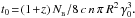
This happens in the observer frame at a time (see, e.g., Dado et al. 2009a, and references therein)  (5)where
Nb is the baryon number of the CB and
R its radius. The rapid decrease of
γ(t) and δ(t) beyond
tb produces a smooth transition (break) around
tb of the observed spectral energy density
Fν(t) ∝ [γ(t)] 3 β−1 [δ(t)] β + 3 ν−β
of the emitted afterglow from a plateau phase to an asymptotic power law decline (e.g.,
Dado et al. 2002, 2009a, and references therein).
(5)where
Nb is the baryon number of the CB and
R its radius. The rapid decrease of
γ(t) and δ(t) beyond
tb produces a smooth transition (break) around
tb of the observed spectral energy density
Fν(t) ∝ [γ(t)] 3 β−1 [δ(t)] β + 3 ν−β
of the emitted afterglow from a plateau phase to an asymptotic power law decline (e.g.,
Dado et al. 2002, 2009a, and references therein).
In the CB model,  and
and
 , respectively.
Consequently, Eq. (5) yields the triple correlation,
, respectively.
Consequently, Eq. (5) yields the triple correlation, ![Mathematical equation: \begin{equation} t'_{\rm b} \propto [E'_{\rm p}\, E_{\rm iso}]^{-1/2}. \label{tbreakepeiso} \end{equation}](/articles/aa/full_html/2013/10/aa21876-13/aa21876-13-eq51.png) (6)Moreover,
substituting the CB model’s approximate binary power law correlation
(6)Moreover,
substituting the CB model’s approximate binary power law correlation
![Mathematical equation: \hbox{$E'_{\rm p} \propto [E_{\rm iso}]^{1/2}$}](/articles/aa/full_html/2013/10/aa21876-13/aa21876-13-eq52.png) into the triple
into the triple  correlation
yields the and
binary
correlations,
correlation
yields the and
binary
correlations, ![Mathematical equation: \begin{equation} t'_{\rm b} \propto [E_{\rm iso}]^{-3/4}\propto [E'_{\rm p}]^{-3/2}, \label{tbreakeiso} \end{equation}](/articles/aa/full_html/2013/10/aa21876-13/aa21876-13-eq54.png) (7)where a prime
indicates the value in the GRB rest frame. Naturally, these approximate correlations are
expected to have a wider spread than the original triple
correlation.
(7)where a prime
indicates the value in the GRB rest frame. Naturally, these approximate correlations are
expected to have a wider spread than the original triple
correlation.
In the case of a wind-like density, which typically extends beyond the end of the glory region at Rg ~ 1016 cm (Dado et al. 2009a,b) and up to Rw ~ 5 × 1017 cm where the wind density decreases below ~mp/cm3 (for the wind parameters listed in Appendix A), the predicted spectral energy flux of the afterglow has the behavior Fν(t) ∝ t−(β + 1) ν−β where β(t) is the spectral index in the observed band (see, e.g., Dado et al. 2009a,b). The observed crossing time of such a wind region is roughly (1 + z) Rw/γ0 δ0, typically <50 (1 + z) s because γ and δ change little during the wind crossing. Beyond the wind region, Fν(t) in the X-ray band has the standard canonical behavior of X-ray afterglows in the CB model in an ISM environment, i.e., with an afterglow smooth break/bend at the end of a plateau phase that satisfies Eq. (7).
3. Comparison with observations
Figure 1 presents the best fit power law to the
observed  correlation
using an unbiased sample of 110 GRBs with known redshift measured before January 1, 2013.
The values of and
Eiso were compiled from communications of the Konus-Wind and
Fermi GBM collaborations to the GCN Circulars Archive (Barthelmy 1997), and from publications by Amati et al. (2007, 2008), Yonetoku et al. (2010), Gruber et al. (2011), Nava et al. (2012), and D’Avanzo et
al. (2012). Using essentially the method advocated by
D’Agostini (2005), we obtained the best fit power law
correlations
correlation
using an unbiased sample of 110 GRBs with known redshift measured before January 1, 2013.
The values of and
Eiso were compiled from communications of the Konus-Wind and
Fermi GBM collaborations to the GCN Circulars Archive (Barthelmy 1997), and from publications by Amati et al. (2007, 2008), Yonetoku et al. (2010), Gruber et al. (2011), Nava et al. (2012), and D’Avanzo et
al. (2012). Using essentially the method advocated by
D’Agostini (2005), we obtained the best fit power law
correlations ![Mathematical equation: \hbox{$E'_{\rm p} \propto [E_{\rm iso}]^{0.54}$}](/articles/aa/full_html/2013/10/aa21876-13/aa21876-13-eq68.png) , in good
agreement with
predicted by the CB model but in disagreement with
, in good
agreement with
predicted by the CB model but in disagreement with  expected in the
conical FB model.
expected in the
conical FB model.
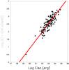 |
Fig. 1 Observed correlation between |
Figure 2 compares the triple correlation
predicted by the
CB model (Eq. (6)) and the observed correlation in 70 Swift GRBs (Evans et
al. 2009) from the above GRB sample, which have a
good Swift/XRT temporal sampling of their X-ray afterglow during the first
day at least following the prompt emission phase and have no superimposed flares. In this
sample the X-ray afterglow of 55 GRBs clearly show a break and no afterglow-break was
observed in 15 GRBs. The upper bound on a possible early time break for the 15 GRBs with no
visible break are indicated. Also shown is the late-time break of the X-ray afterglow of GRB
980425, which was measured with Chandra (Kouveliotou et al. 2004). In order not to bias the values of tb by the CB
model fits, the break times were taken to be the times of the first break with
α(t < tb) < α(t > tb)
obtained from a broken power law fit to the GRB X-ray afterglow measured with the
Swift/XRT and reported in the Leicester XRT GRB catalog (Evans et al.
2009) or from the smoothly broken power law fits of
Margutti et al. (2013). The Spearman rank
(correlation coefficient) of the triple correlation  for the
subsample of 55 GRBs with a visible break is r = −0.74 corresponding to a
chance probability less than 1.4 × 10⁻¹⁰. The best fit triple correlation
for the
subsample of 55 GRBs with a visible break is r = −0.74 corresponding to a
chance probability less than 1.4 × 10⁻¹⁰. The best fit triple correlation
![Mathematical equation: \hbox{$t'_{\rm b} \propto [E'_{\rm p}\, E_{\rm iso}]^q $}](/articles/aa/full_html/2013/10/aa21876-13/aa21876-13-eq75.png) that was obtained
for the subsample of 55 GRBs, using essentially the maximum likelihood method advocated by
D’Agostini (2005), yields
q = −0.58 ± 0.04.
that was obtained
for the subsample of 55 GRBs, using essentially the maximum likelihood method advocated by
D’Agostini (2005), yields
q = −0.58 ± 0.04.
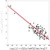 |
Fig. 2 Observed triple correlations |
The approximate binary correlations and
that were
obtained by substituting the CB model predicted correlation
in
the triple correlation (Eq. (6)) are
compared to the observational data in Figs. 3 and 4, respectively. GRB 980425 was excluded from the GRB
sample because in the CB model is
only satisfied by ordinary GRBs where
θ ≈ 1/γ, while far-off axis GRBs,
such as 980 425, with θ ≫ 1/γ, satisfy
![Mathematical equation: \hbox{$E'_{\rm p}\propto [E_{\rm iso}]^{1/3}$}](/articles/aa/full_html/2013/10/aa21876-13/aa21876-13-eq81.png) ;
i.e., they are outliers with respect to the assumed
correlation. The Spearman ranks of the observed and
correlations
are − 0.49 and −0.63 with chance probabilities less than 4.5 × 10⁻⁴ and
1.0 × 10⁻⁶, respectively, and as expected (in the CB model), they are larger
than that of the
;
i.e., they are outliers with respect to the assumed
correlation. The Spearman ranks of the observed and
correlations
are − 0.49 and −0.63 with chance probabilities less than 4.5 × 10⁻⁴ and
1.0 × 10⁻⁶, respectively, and as expected (in the CB model), they are larger
than that of the  correlations. The best fit power law indices of the , and
correlations
are −0.70 ± 0.06, and −1.64 ± 0.04 , respectively, consistent with their
predicted values by the CB model, −0.75 and −1.50, respectively.
correlations. The best fit power law indices of the , and
correlations
are −0.70 ± 0.06, and −1.64 ± 0.04 , respectively, consistent with their
predicted values by the CB model, −0.75 and −1.50, respectively.
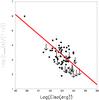 |
Fig. 3 Comparison between the binary correlation |
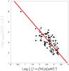 |
Fig. 4 Comparison between the binary correlation |
A comparison between the best fit indices of the break-time power law correlations and
those expected in the CB and FB models is summarized in Table 1 for the sample of 55 Swift GRBs with a visible
afterglow break. As can be seen from Table 1, the
values of the power law correlation indices predicted by the CB model are consistent with
those obtained from the best fits. The best fit indices, 0.54 ± 0.01, −0.69 ± 0.06, and
−1.62 ± 0.04 of the observed ,
and
power law
correlations, however, are at odds with the values 1, −1, and −1, respectively, expected
in the conical FB model. While the
χ2/d.o.f.
of the predicted correlations by the CB model differ from those of the best fits by less
than 1/d.o.f., the
χ2/d.o.f.
of the predicted correlations by the FB model differ by much higher values, as summarized in
Table 2.
The correlations satisfied by  imply that GRBs
with very high Eiso and/or
have a break at
small , which is
hidden under the tail of the prompt emission or precedes the start of the
Swift/XRT follow-up observations (Dado et al. 2007). Indeed, the X-ray afterglow of all the 15 GRBs in the sample,
which have a very high
imply that GRBs
with very high Eiso and/or
have a break at
small , which is
hidden under the tail of the prompt emission or precedes the start of the
Swift/XRT follow-up observations (Dado et al. 2007). Indeed, the X-ray afterglow of all the 15 GRBs in the sample,
which have a very high  , have a single
power law decline consistent with the post-break power law decline predicted by the CB model
(see, e.g., Dado et al. 2007, 2009a). For such GRBs, the observations only provide upper bounds for the
break times of their X-ray afterglows.
, have a single
power law decline consistent with the post-break power law decline predicted by the CB model
(see, e.g., Dado et al. 2007, 2009a). For such GRBs, the observations only provide upper bounds for the
break times of their X-ray afterglows.
Summary of the observed power law correlations between
,
Eiso and and their power
law indices expected in the cannonball (CB) and collimated fireball (FB) models.
The χ2/d.o.f. statistic for the best fit power law
correlations between ,
Eiso and and for the
correlations predicted by the CB and collimated FB models.
However, for most of the 15 GRBs with only an upper bound on their afterglow break time, which are indicated by down pointing errors in Figs. 2−4, an early break time value was extracted from a CB model fit to the entire X-ray light curve, which includes the fast decline phase of the prompt emission and the afterglow component (see, e.g., Dado et al. 2009a,b). Replacement of the upper bounds by the CB model fitted break times (which could have biased the break times values) and their inclusion in the best fits had very little effect on the values of the best fit power law indices and their errors.
4. Conclusions and discussion
Correlations and closure relations between GRB properties that are predicted by GRB models
allow parameter-free tests of such models. In particular, comparison between the observed
and predicted correlations between the jet break in the X-ray afterglow of GRBs and the
prompt gamma-ray emission, like the correlation,
allow another critical test of the conical FB model and the CB model of GRBs. Although the
jet break in the afterglow of GRBs has been the flagship of the conical FB model, the
observed correlations between the jet break in the X-ray afterglow of GRBs measured with the
Swift/XRT and their prompt gamma-ray emission are inconsistent with those
expected in the conical FB model. This failure, perhaps, is not a surprise since the
observed jet-breaks were found before to be chromatic, the predicted pre- and post-break
temporal behaviors and closure relations were found to be badly violated, and the observed
change in slope across the breaks is not the one predicted. The replacement of the
approximate analytical estimates in the conical FB model (Sari et al. 1999) by more exact hydrodynamical calculations (e.g. van Eerten
& MacFadyen 2013) does not change the
situation. They neither reproduce the observed correlations, nor do they remove the
discrepancies between the predicted and observed pre-break and post break behaviors of the
afterglows. These failures provide additional evidence that GRBs and their afterglows are
not produced by conical jets, the so called collimated FBs.
In contrast, the correlations between the deceleration break in the afterglow of GRBs and
their prompt γ-ray emission predicted by the CB model are in good agreement
with those observed, as shown in Figs. 1−4. The correlations between the break and other afterglow
properties predicted by the CB model (Dado & Dar 2012b), as well as the pre-break and post-break behaviors of the light curves of
the X-ray afterglow, were shown to accord well with the observations (e.g., Dado et al.
2009a,b; Dado & Dar 2012a). Moreover, in the CB model, the
 anti-correlation noted by Stratta et al. (2009), is a
simple consequence of beaming and the detection threshold, which enrich the low
z GRB sample with far-off-axis soft GRBs and X-ray flashes (e.g., Dado et
al. 2004) relative to the high z
events that must be much harder and energetic in order to be detected. These selection
effects that produce the effective
anti-correlation noted by Stratta et al. (2009), is a
simple consequence of beaming and the detection threshold, which enrich the low
z GRB sample with far-off-axis soft GRBs and X-ray flashes (e.g., Dado et
al. 2004) relative to the high z
events that must be much harder and energetic in order to be detected. These selection
effects that produce the effective  and
⟨ Eiso(z) ⟩ − z
“correlations” result in an effective
and
⟨ Eiso(z) ⟩ − z
“correlations” result in an effective  ’anti-correlation’ (Dado
& Dar, in prep.).
’anti-correlation’ (Dado
& Dar, in prep.).
The solid angle of a conical shell is Ωj = 2 π (1 − cosθj), which yields a beaming factor fb = 2 π (1 − cosθj)/4 π = (1 − cosθj)/2, and not fb = (1 − cosθj) that is widely used in the GRB literature.
Acknowledgments
We thank an anonymous referee for useful comments and suggestions.
References
- Amati, L., Della Valle, M., Frontera, F., et al. 2007, A&A, 463, 913A [NASA ADS] [CrossRef] [EDP Sciences] [Google Scholar]
- Amati, L., Guidorzi, C., Frontera, F., et al. 2008, MNRAS, 391, 577 [NASA ADS] [CrossRef] [MathSciNet] [Google Scholar]
- Barthelmy, S. 1997, http://gcn.gsfc.nasa.gov/gcn_main.html [Google Scholar]
- Beuermann, Hessman, F. V., Reinsch, K., et al. 1999, A&A, 352, L26 [NASA ADS] [Google Scholar]
- Costa, E., Frontera, F., Heise, J., et al. 1997, Nature, 387, 783 [NASA ADS] [CrossRef] [Google Scholar]
- Covino, S., Malesani, D., Tagliaferri, G., et al. 2006, IL Nuovo Cimento B, 121, 1171 [NASA ADS] [Google Scholar]
- Curran, P. A., van der Horst, A. J., & Wijers, R. A. M. J. 2008, MNRAS, 386, 859 [NASA ADS] [CrossRef] [Google Scholar]
- Dado, S., & Dar, A. 2012a, ApJ, 761, 148 [NASA ADS] [CrossRef] [Google Scholar]
- Dado, S., & Dar, A. 2012b, ApJ, in press [arXiv:1203.5886] [Google Scholar]
- Dado, S., Dar, A., & De Rújula, A. 2002, A&A, 388, 1079 [NASA ADS] [CrossRef] [EDP Sciences] [Google Scholar]
- Dado, S., Dar, A., & De Rújula, A. 2004, A&A, 422, 2004 [Google Scholar]
- Dado, S., Dar, A., & De Rújula, A. 2007, ApJ, 663, 400 [NASA ADS] [CrossRef] [Google Scholar]
- Dado, S., Dar, A., & De Rújula, A. 2009a, ApJ, 696, 994 [NASA ADS] [CrossRef] [Google Scholar]
- Dado, S., Dar, A., & De Rújula, A. 2009b, ApJ, 693, 311 [NASA ADS] [CrossRef] [Google Scholar]
- D’Agostini, G. 2005 [arXiv:astro-ph/0511182] [Google Scholar]
- Dar, A. 1998, ApJ, 500, L93 [NASA ADS] [CrossRef] [Google Scholar]
- Dar, A., & De Rújula A. 2000 [arXiv:astro-ph/0008474] [Google Scholar]
- Dar, A., & De Rújula A., 2004, Phys. Rep. 405, 203 [NASA ADS] [CrossRef] [Google Scholar]
- D’Avanzo, P., Salvaterra, R., Sbarufatti, B., et al. 2012, MNRAS, 425, 506 [NASA ADS] [CrossRef] [Google Scholar]
- Evans, P. A., Beardmore, A. P., Page, K. L., et al. 2009, MNRAS, 397, 1177 [NASA ADS] [CrossRef] [Google Scholar]
- Frail, D. A., Kulkarni, S. R., Nicastro, L., et al. 1997, Nature, 389, 261 [NASA ADS] [CrossRef] [Google Scholar]
- Frail, D. A., Kulkarni, S. R., Sari, R., et al. 2001, ApJ, 562, L55 [NASA ADS] [CrossRef] [Google Scholar]
- Fruchter, A. S., Thorsett, S. E., Metzger, M. R. A., et al. 1999, ApJ, 519, L13 [NASA ADS] [CrossRef] [Google Scholar]
- Goodman, J., 1986, ApJ, 308, L47 [NASA ADS] [CrossRef] [Google Scholar]
- Goodman, J., Dar, A., & Nussinov, S. 1987, ApJ, 314, L7 [NASA ADS] [CrossRef] [Google Scholar]
- Gruber, D., Greiner, J., von Kienlin, A., et al. 2011, A&A, 531A, 20 [Google Scholar]
- Harrison, F. A., Bloom, J. S., Frail, D. A., et al. 1999, ApJ, 523, L121 [NASA ADS] [CrossRef] [Google Scholar]
- Katz, J. 1994, ApJ, 432, L107 [NASA ADS] [CrossRef] [Google Scholar]
- Kocevski, D., & Butler, N. 2008, ApJ, 680, 531 [NASA ADS] [CrossRef] [Google Scholar]
- Kouveliotou, C., Woosley, S. E., Patel, S. K., et al. 2004, ApJ, 608, 872 [NASA ADS] [CrossRef] [Google Scholar]
- Kulkarni, S. R., Djorgovski, S. G., Odewahn, S. C., et al. 1999, Nature, 398, 389 [NASA ADS] [CrossRef] [Google Scholar]
- Liang, E. W., Racusin, J.L., Zhang, B., et al. 2008, ApJ, 675, L528 [NASA ADS] [CrossRef] [Google Scholar]
- Margutti, R., Zaninoni, E., Bernardini, M. G., et al. 2013, MNRAS, 428, 729 [NASA ADS] [CrossRef] [Google Scholar]
- Meegan, Fishman, G. J., Wilson, R. B., et al. 1992, Nature, 355, 143 [NASA ADS] [CrossRef] [Google Scholar]
- Meszaros, P., & Rees, M. J. 1997, ApJ, 476, 232 [NASA ADS] [CrossRef] [Google Scholar]
- Metzger, M. R., Djorgovski, S. G., Kulkarni, S. R., et al. 1997, Nature, 387, 878 [NASA ADS] [CrossRef] [Google Scholar]
- Mao, S., & Paczynski, B. 1992, ApJ, 388, L45 [NASA ADS] [CrossRef] [Google Scholar]
- Nava, L., Salvaterra, R., Ghirlanda, G., et al. 2012, MNRAS, 421, 1256 [NASA ADS] [CrossRef] [MathSciNet] [Google Scholar]
- Nousek, J. A., Kouveliotou, C., Grupe, D., et al. 2006, ApJ, 642, 389 [NASA ADS] [CrossRef] [Google Scholar]
- Paczynski, B. 1986, ApJ, 308, L43 [NASA ADS] [CrossRef] [Google Scholar]
- Paczynski, B., & Rhoads, J. E. 1993, ApJ, 418, L5 [NASA ADS] [CrossRef] [Google Scholar]
- Panaitescu, A., Mészáros, P., Burrows, D., et al. 2006, MNRAS, 369, 2059 [NASA ADS] [CrossRef] [Google Scholar]
- Piran, T. 1999, Phys. Rep. 314, 575 [NASA ADS] [CrossRef] [Google Scholar]
- Piran, T. 2000, Phys. Rep. 333, 529 [NASA ADS] [CrossRef] [Google Scholar]
- Racusin, J. L., Liang, E. W., Burrows, D. N., et al. 2009, ApJ, 698, 43 [NASA ADS] [CrossRef] [Google Scholar]
- Sahu, K. C., Livio, M., Petro, L., et al. 1997, Nature, 387, 476 [NASA ADS] [CrossRef] [Google Scholar]
- Sari, R., Piran, T., & Halpern, J. P. 1999, ApJ, 519, L17 [NASA ADS] [CrossRef] [Google Scholar]
- Shaviv, N. J., & Dar, A. 1995, ApJ, 447, 863 [NASA ADS] [CrossRef] [Google Scholar]
- Stratta, G., Guetta, D., D’Elia, V., et al. 2009, A&A, 494, L9 [NASA ADS] [CrossRef] [EDP Sciences] [Google Scholar]
- Van Eerten, H. J., MacFadyen, A. I., & Zhang, W. 2011, AIP Conf. Proc., 1358, 173 [NASA ADS] [CrossRef] [Google Scholar]
- van Eerten, F., & MacFadyen, A. 2013, ApJ, 767, 141 [NASA ADS] [CrossRef] [Google Scholar]
- van Paradijs, J., Groot, P. J., Galama, T., et al. 1997, Nature, 386, 686 [NASA ADS] [CrossRef] [Google Scholar]
- Wijers, R. A. M. J., Rees, J., & Meszaros, P. 1997, MNRAS, 288, L51 [NASA ADS] [CrossRef] [Google Scholar]
- Yonetoku, D., Murakami, T., Tsutsui, R., et al. 2010, PASJ, 62, 1495 [NASA ADS] [Google Scholar]
Appendix A: Ballistic conical shells
Consider the deceleration of a highly relativistic conical shell of a solid angle
 that
expands radially and decelerates by sweeping in the medium in front of it. Assuming a
plastic collision and neglecting radiation losses, relativistic energy-momentum
conservation, d(M γ) = 0, can be written as,
that
expands radially and decelerates by sweeping in the medium in front of it. Assuming a
plastic collision and neglecting radiation losses, relativistic energy-momentum
conservation, d(M γ) = 0, can be written as,
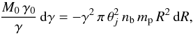 (A.1)where
M(t) = M0 γ(0)/γ
is the mass of the jet, M0 = M(0),
γ0 = γ(0), nb
is the constant baryon density of the external medium, and
R(t) is the radius of the conical shell. Equation
(A.1) yields
(A.1)where
M(t) = M0 γ(0)/γ
is the mass of the jet, M0 = M(0),
γ0 = γ(0), nb
is the constant baryon density of the external medium, and
R(t) is the radius of the conical shell. Equation
(A.1) yields ![Mathematical equation: \appendix \setcounter{section}{1} \begin{equation} [R^3-R_0^3]= {3\, M_0\,\gamma_0 \over 2\,\pi\,\theta_j^2\,n\,m_{\rm p}}\, \left[{1\over \gamma^2}-{1\over \gamma_0^2}\right]\cdot \label{Rgamma} \end{equation}](/articles/aa/full_html/2013/10/aa21876-13/aa21876-13-eq122.png) (A.2)In the conical FB model,
ordinary GRBs have
(A.2)In the conical FB model,
ordinary GRBs have  , whereas
 at the break-time
in the GRB
rest frame corresponding to a break-time tb in the observer
frame. Consequently, Eq. (A.1) implies that the radius of the conical shell at
is given by
at the break-time
in the GRB
rest frame corresponding to a break-time tb in the observer
frame. Consequently, Eq. (A.1) implies that the radius of the conical shell at
is given by
![Mathematical equation: \appendix \setcounter{section}{1} \begin{equation} R_{\rm b}=R(t'_{\rm b})\approx \left[{3\,E_{\rm k}\over 2\,\pi\, n\, m_{\rm p}\,c^2}\right]^{1/3}, \label{Rb} \end{equation}](/articles/aa/full_html/2013/10/aa21876-13/aa21876-13-eq125.png) (A.3)where
Ek ≃ M0 γ0 c2
is the kinetic energy of the conical ejecta. Equation (A.1) also yields the asymptotic
behavior
R ≈ c t′ ≈ Rb [γ(t′)/γb] −2/3,
which is already reached well before . Because of
time aberration and cosmic expansion, the on-axis observer’s time interval
dt that corresponds to the time interval
dt′ = dR/c
in the GRB rest frame is given by
dt = (1 + z) dt′/2 γ2.
Consequently, γ(t′) has the asymptotic
behavior
γb (t/tb)−3/8
where the observed on-axis break-time is given by
(A.3)where
Ek ≃ M0 γ0 c2
is the kinetic energy of the conical ejecta. Equation (A.1) also yields the asymptotic
behavior
R ≈ c t′ ≈ Rb [γ(t′)/γb] −2/3,
which is already reached well before . Because of
time aberration and cosmic expansion, the on-axis observer’s time interval
dt that corresponds to the time interval
dt′ = dR/c
in the GRB rest frame is given by
dt = (1 + z) dt′/2 γ2.
Consequently, γ(t′) has the asymptotic
behavior
γb (t/tb)−3/8
where the observed on-axis break-time is given by 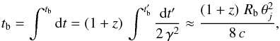 (A.4)and where we have
assumed that most of the contribution to the integral comes from times when
(A.4)and where we have
assumed that most of the contribution to the integral comes from times when
 is
already a good approximation.
is
already a good approximation.
If the total gamma-ray energy emitted in GRBs is a constant fraction of the initial
kinetic energy of the conical shell,
Eγ = η Ek,
which in the conical FB model is related to the isotropic equivalent gamma-ray energy
Eiso of the GRB by1 then
then
![Mathematical equation: \appendix \setcounter{section}{1} \begin{equation} t_{\rm b} ={(1+z)\over 16\,c} \left[{3\,E_{\rm iso}\over \pi\, \eta\, n\, m_{\rm p}\, c^2} \right]^{1/3}\, \theta_j^{8/3}. \label{tb2} \end{equation}](/articles/aa/full_html/2013/10/aa21876-13/aa21876-13-eq137.png) (A.5)Equations (A.4) and
(A.5) were used by Sari et al. (1999) to represent
conical jets with lateral expansion.
(A.5)Equations (A.4) and
(A.5) were used by Sari et al. (1999) to represent
conical jets with lateral expansion.
A distant observer sees only the beamed radiation from an area
R2 π/γ2
along the line of sight of a spherical shell or a conical shell. Consequently, as long as
γ(t) > 1/θj
the observed afterglows from a conical FB or an isotropic FB have the same visible area.
Beyond the break the visible area of a spherical FB continues to be
≈R2π/γ2,
while that of a conical shell becomes ≈ . Hence the
lightcurve of the afterglow of the conical FB beyond the break is steeper by their ratio
. Hence the
lightcurve of the afterglow of the conical FB beyond the break is steeper by their ratio
 ,
where we used the asymptotic behavior
γ(t) = γb (t/tb)−3/8
in a constant density environment and
γb = 1/θj.
This steepening of the power law decline by Δα = 0.75 across the break
independent of β is different from what was derived by Sari et al. (1999) for a spreading jet.
,
where we used the asymptotic behavior
γ(t) = γb (t/tb)−3/8
in a constant density environment and
γb = 1/θj.
This steepening of the power law decline by Δα = 0.75 across the break
independent of β is different from what was derived by Sari et al. (1999) for a spreading jet.
The smooth transition between the pre- and post-break power laws can also be derived more
rigorously: relativistic beaming and Doppler boosting modulates the observed emission from
every point on the conical shell by a factor δ1 + Γ where
δ = 1/γ (1 − β cosθ)
is the Doppler factor on the shell at an angle θ relative to the line of
sight to the observer,
β = v/c, and Γ is
the photon spectral index of the radiation. For isotropic medium, isotropic conical shell,
and isotropic expansion, this is the only dependence of the received radiation on the line
of sight to the observer. Consequently, the observed energy-flux (at a given energy) of
photons emitted simultaneosly by the conical shell is modulated by the factor
![Mathematical equation: \appendix \setcounter{section}{1} \begin{equation} I(\gamma,\theta_j)=2\pi\int \delta^{\Gamma+1} {\rm d}\cos\theta ={2\,\pi \over \beta\,\gamma\,\Gamma} \left[{1\over(1\!-\!\beta)^\Gamma}-{1\over (1\!-\!\beta\cos\theta_j)^\Gamma}\right]\cdot \label{I2} \end{equation}](/articles/aa/full_html/2013/10/aa21876-13/aa21876-13-eq151.png) (A.6)The difference in arrival
times of photons emitted simultaneously from the conical shell was ignored in the above
analytical estimates of the break time and the spectral index change across the break. The
spread in arrival times has no effect on Eiso, it is
Δt ≈ R/2 c γ2
before the break and
(A.6)The difference in arrival
times of photons emitted simultaneously from the conical shell was ignored in the above
analytical estimates of the break time and the spectral index change across the break. The
spread in arrival times has no effect on Eiso, it is
Δt ≈ R/2 c γ2
before the break and  after the break. Thus,
Δt is roughly four times higher than t before the
break but less than t by a factor
after the break. Thus,
Δt is roughly four times higher than t before the
break but less than t by a factor  at late times. The spread in
arrival time that has a negligible effect on Eiso and
Δα cannot be neglected in estimating tb.
The same conclusion is also valid for the effects of off-axis viewing when the viewing
angle θ is not negligible compared to
θj. Generally, the effects of off-axis
viewing and the spread in arrival time require numerical integrations (e.g., van Eerten
& MacFadyen 2013) and make the widely used
simple relation, Eq. (A.4) a very rough estimate.
at late times. The spread in
arrival time that has a negligible effect on Eiso and
Δα cannot be neglected in estimating tb.
The same conclusion is also valid for the effects of off-axis viewing when the viewing
angle θ is not negligible compared to
θj. Generally, the effects of off-axis
viewing and the spread in arrival time require numerical integrations (e.g., van Eerten
& MacFadyen 2013) and make the widely used
simple relation, Eq. (A.4) a very rough estimate.
If the typical circumburst region of LGRBs is the wind region of a Wolf Rayet star that
blows a constant wind, then its density profile is 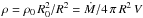 where the typical mass-loss
rate Ṁ ~ 10-4 M⊙y-1
and the typical wind velocity V ~ 1000 km s-1 yield
where the typical mass-loss
rate Ṁ ~ 10-4 M⊙y-1
and the typical wind velocity V ~ 1000 km s-1 yield
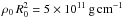 .
The replacement of
nb mp R2
with
.
The replacement of
nb mp R2
with  in the Eq. (A.1),
and repetition of the derivations of the break-time correlations for a constant density,
yield, for γ θ = 1,
in the Eq. (A.1),
and repetition of the derivations of the break-time correlations for a constant density,
yield, for γ θ = 1, 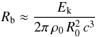 (A.7)i.e.,
a typical Rb ≈ 3.5 × 10¹⁶ independent of
θ, and
(A.7)i.e.,
a typical Rb ≈ 3.5 × 10¹⁶ independent of
θ, and 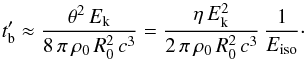 (A.8)The break-time
power law correlations for ISM and wind-like density profiles thus have identical power
law indices, i.e.,
(A.8)The break-time
power law correlations for ISM and wind-like density profiles thus have identical power
law indices, i.e.,  .
.
Appendix B: Ballistic cannonballs
In the CB model the electrons that enter the CB are Fermi-accelerated, and they cool
rapidly by synchrotron radiation (SR). This radiation is isotropic in the CB’s rest frame
and has a smoothly broken power law spectrum with a characteristic bend/break frequency,
which is the typical synchrotron frequency radiated by the ISM electrons that enter the CB
at time t with a relative Lorentz factor
γ(t). In the observer frame, the emitted photons are
beamed into a narrow cone along the CB’s direction of motion by its highly relativistic
bulk motion, their arrival times are aberrated and their energies are boosted by its bulk
motion Doppler factor δ and redshifted by the cosmic expansion during
their travel time to the observer. For the X-ray band that is well above the break
frequency, the CB model yields the spectral energy density (see, e.g., Eq. (26) in Dado et
al. 2009a), ![Mathematical equation: \appendix \setcounter{section}{2} \begin{equation} F_{\nu} \propto n^{(\beta_{\rm X}+1)/2}\, [\gamma(t)]^{3\,\beta_{\rm X}-1}\, \left[\delta(t)\right]^{\beta_{\rm X}+3}\, \nu^{-\beta_{\rm X}}. \label{Fnu} \end{equation}](/articles/aa/full_html/2013/10/aa21876-13/aa21876-13-eq168.png) (B.1)For a CB of a baryon
number
(B.1)For a CB of a baryon
number  , a
constant or slowly expanding radius R and an initial Lorentz factor
γ0 = γ(0) ≫ 1, which propagates in an ISM
of a constant density nb, relativistic energy-momentum
conservation yields the deceleration law (Dado et al. 2009b, and references therein)
, a
constant or slowly expanding radius R and an initial Lorentz factor
γ0 = γ(0) ≫ 1, which propagates in an ISM
of a constant density nb, relativistic energy-momentum
conservation yields the deceleration law (Dado et al. 2009b, and references therein)
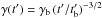
![Mathematical equation: \appendix \setcounter{section}{2} \begin{equation} \gamma(t) = {\gamma_0\over \left[\sqrt{(1+\theta^2\,\gamma_0^2)^2 +t/t_0} - \theta^2\,\gamma_0^2\right]^{1/2}}, \end{equation}](/articles/aa/full_html/2013/10/aa21876-13/aa21876-13-eq171.png) (B.2)where
(B.2)where
 As long
as
As long
as  ,
γ(t) and δ(t) change
rather slowly with t, which generates the plateau phase of
Fν(t) of canonical X-ray
AGs that was predicted by the CB model (see, e.g., Dado et al. 2002, Figs. 6, 27−33) and later observed with Swift
(Nousek et al. 2005). For
t ≫ tb,
γ(t) → γ0(t/tb)−1/4,
[γ(t)θ] 2 becomes ≪1 and
δ ≈ 2 γ(t), which result in a
post-break power law decline
,
γ(t) and δ(t) change
rather slowly with t, which generates the plateau phase of
Fν(t) of canonical X-ray
AGs that was predicted by the CB model (see, e.g., Dado et al. 2002, Figs. 6, 27−33) and later observed with Swift
(Nousek et al. 2005). For
t ≫ tb,
γ(t) → γ0(t/tb)−1/4,
[γ(t)θ] 2 becomes ≪1 and
δ ≈ 2 γ(t), which result in a
post-break power law decline  (B.3)Thus, in the CB model,
the asymptotic post-break decline of the X-ray afterglow of a single CB in an ISM
environment satisfies the closure relation
αX = βX + 1/2 = ΓX −1/2
(or αX = βX = ΓX − 1
for a shot-gun configuration of CBs) independent of the pre-break behavior, which strongly
depends on viewing angle (e.g., Dado & Dar 2012a).
(B.3)Thus, in the CB model,
the asymptotic post-break decline of the X-ray afterglow of a single CB in an ISM
environment satisfies the closure relation
αX = βX + 1/2 = ΓX −1/2
(or αX = βX = ΓX − 1
for a shot-gun configuration of CBs) independent of the pre-break behavior, which strongly
depends on viewing angle (e.g., Dado & Dar 2012a).
All Tables
Summary of the observed power law correlations between
,
Eiso and and their power
law indices expected in the cannonball (CB) and collimated fireball (FB) models.
The χ2/d.o.f. statistic for the best fit power law
correlations between ,
Eiso and and for the
correlations predicted by the CB and collimated FB models.
All Figures
|
Fig. 1 Observed correlation between |
| In the text | |
|
Fig. 2 Observed triple correlations |
| In the text | |
|
Fig. 3 Comparison between the binary correlation |
| In the text | |
|
Fig. 4 Comparison between the binary correlation |
| In the text | |
Current usage metrics show cumulative count of Article Views (full-text article views including HTML views, PDF and ePub downloads, according to the available data) and Abstracts Views on Vision4Press platform.
Data correspond to usage on the plateform after 2015. The current usage metrics is available 48-96 hours after online publication and is updated daily on week days.
Initial download of the metrics may take a while.