| Issue |
A&A
Volume 557, September 2013
|
|
|---|---|---|
| Article Number | A120 | |
| Number of page(s) | 8 | |
| Section | Interstellar and circumstellar matter | |
| DOI | https://doi.org/10.1051/0004-6361/201321760 | |
| Published online | 18 September 2013 | |
High-fidelity view of the structure and fragmentation of the high-mass, filamentary IRDC G11.11-0.12
Max-Planck-Institute for Astronomy, Königstuhl 17, 69117 Heidelberg, Germany
e-mail: This email address is being protected from spambots. You need JavaScript enabled to view it.
Received: 23 April 2013
Accepted: 13 June 2013
Abstract
Star formation in molecular clouds is intimately linked to their internal mass distribution. We present an unprecedentedly detailed analysis of the column density structure of a high-mass, filamentary molecular cloud, namely IRDC G11.11-0.12 (G11). We use two novel column density mapping techniques: high-resolution (FWHM = 2″, or ~0.035 pc) dust extinction mapping in near- and mid-infrared, and dust emission mapping with the Herschel satellite. These two completely independent techniques yield a strikingly good agreement, highlighting their complementarity and robustness. We first analyze the dense gas mass fraction and linear mass density of G11. We show that G11 has a top heavy mass distribution and has a linear mass density (Ml ~ 600 M⊙ pc-1) that greatly exceeds the critical value of a self-gravitating, non-turbulent cylinder. These properties make G11 analogous to the Orion A cloud, despite its low star-forming activity. This suggests that the amount of dense gas in molecular clouds is more closely connected to environmental parameters or global processes than to the star-forming efficiency of the cloud. We then examine hierarchical fragmentation in G11 over a wide range of size-scales and densities. We show that at scales 0.5 pc ≳ l ≳ 8 pc, the fragmentation of G11 is in agreement with that of a self-gravitating cylinder. At scales smaller than l ≲ 0.5 pc, the results agree better with spherical Jeans’ fragmentation. One possible explanation for the change in fragmentation characteristics is the size-scale-dependent collapse time-scale that results from the finite size of real molecular clouds: at scales l ≲ 0.5 pc, fragmentation becomes sufficiently rapid to be unaffected by global instabilities.
Key words: ISM: clouds / ISM: structure / stars: formation / dust, extinction
© ESO, 2013
1. Introduction
Measuring mass distributions of molecular clouds is of crucial importance for understanding processes that regulate star formation (Hennebelle & Falgarone 2012). However, probing the entire wide range of (column) densities that molecular clouds show, at a resolution that resolves their substructure, is an observational challenge. This is especially true for high-mass clouds that potentially harbor precursors of high-mass stars because of their higher column densities and larger distances. Owing to these difficulties, a global description of the relation between molecular cloud structure and star formation is still elusive.
The Herschel satellite (Pilbratt et al. 2010) provides an outstanding tool to study the structure of high-mass molecular clouds at different scales (e.g., Beuther et al. 2010; Schneider et al. 2012), thanks to its high mapping speed and dynamic range. In particular, early studies employing Herschel data have signified the role of filamentary structures as an important pathway toward star formation (e.g., André et al. 2010). However, Herschel observations only provide column density data in a spatial resolution of ~25″ (~0.4 pc at 3.5 kpc), while molecular clouds show fragmentation down to at least ≲0.03 pc (e.g., Stanke et al. 2006; Peretto & Fuller 2009).
We have developed an alternative, novel technique to map column densities in infrared dark clouds (IRDCs) using dust extinction measurements in near- and mid-infrared (NIR and MIR, Kainulainen & Tan 2013). The technique takes advantage of the high resolution of the Spitzer 8 μm images (full width at half maximum, FWHM = 2″) and of the relatively good sensitivity of NIR-based extinction data (cf., Kainulainen et al. 2011). When combined, these data can provide unique, high-resolution column density data that cover a relatively wide range of column densities, N(H2) ≈ 2 − 150 × 1021 cm-2. Importantly, the assumptions on which the technique is based are completely different to those employed with dust emission techniques. This makes dust extinction data highly complementary to Herschel data, in addition to the advantage that it provides more than ten times higher spatial resolution.
The IRDC G11.11-0.12 (G11) is an excellent target for studying the structure of a young, high-mass cloud at the onset of star formation. The ~30 pc long filamentary cloud contains a large reservoir of cold gas as evidenced by its MIR and sub-mm properties (Carey et al. 2000; Johnstone et al. 2003; Henning et al. 2010). It harbors 19 Herschel point sources, most of which contain 24 μm sources indicating the presence of a protostar (Henning et al. 2010; Ragan et al. 2012). It also contains one possible high-mass star-forming core (Pillai et al. 2006a).
In this paper, we present an analysis of the density structure of G11 using high-resolution (FWHM = 2″ corresponding to 0.035 pc assuming d = 3.6 kpc) dust extinction data and Herschel dust emission data. The data allow us to cover, for the first time in an IRDC, simultaneously the scales from tenth-of-a-parsec cores to the large-scale, tenuous envelope of the cloud.
2. Observations
2.1. High-dynamic-range dust extinction data
We derived column density data for G11 using the extinction mapping technique presented by Kainulainen & Tan (2013). The technique combines MIR (8 μm) surface brightness data with NIR (JHK) photometry of stars. We derived an 8 μm optical depth (τ8 μm) map of G11 using the Spitzer/GLIMPSE data (Benjamin et al. 2003) and the approach detailed in Ragan et al. (2009). Then, we derived a NIR extinction map using data from the UKIRT/Galactic Plane Survey (Lawrence et al. 2007) and the procedure described in Kainulainen et al. (2011). The data sets were then combined as described in Kainulainen & Tan (2013). For the procedure, it is necessary to adopt the relative dust opacity law between the JHK bands and 8 μm. We adopted the relations (Cardelli et al. 1989; Ossenkopf & Henning 1994)  (1)Finally, the optical depths were used to estimate column densities via the conversion (Savage et al. 1977; Bohlin et al. 1978)
  (2)Figure 1 shows the resulting column density map of G11. It has the spatial resolution of 2″ and 3-σ sensitivity of N(H2) ≈ 2 × 1021 cm-2. The zero-point uncertainty of the map is about σ0,N(H2) ≈ 1 × 1021 cm-2 (cf., Kainulainen et al. 2011).
2.2. Herschel data
We derived column densities in G11 using Herschel data. The data were obtained under the Earliest Phases of Star formation guaranteed time key programme (PI: O. Krause) and are described in Ragan et al. (2012). The data were processed to level 1 using HIPE (Ott 2010), developer build 10.0(2538), calibration trees 42 (PACS) and 10.0 (SPIRE). We generated final maps using Scanamorphos version 20 (Roussel 2012), with the “galactic” option, and included the non-zero-acceleration telescope turn-around data. Using the spectral energy distribution fitting method (Launhardt et al. 2013), we computed N(H2) for positions with emission in at least four bands of the Herschel 70, 100, 160, 250, and 350 μm data and 870 μm ATLASGAL data (Schuller et al. 2009). All maps were first convolved to the resolution of the 350 μm maps ( ) and re-gridded to match the 6″-per-pixel SPIRE grid scale. We present the resulting column density and temperature maps in Ragan et al. (in prep.).
Since we later compare the Herschel-derived column densities with the extinction-derived ones, it is important to ascertain that the dust opacities (that directly affect the column densities) are chosen consistently from sub-mm to NIR. Dust opacities are not very well constrained, as the range of plausible models is at least a factor of five in sub-mm and two in 8 μm and NIR (shown in Fig. A.1). The effective dust opacities used in calculating column densities from NIR and 8 μm (see Kainulainen & Tan 2013) are close to the means of the models shown in Fig. A.1. Therefore, we choose to use the mean values from the models also in calculating the column densities from Herschel data (see Fig. A.1). These values are formally closest to the Ossenkopf & Henning (1994) dust model without dust coagulation.
The column density/temperature fitting technique we employ (Launhardt et al. 2013) does not take into account that significant amount of the detected emission may result from the extended, diffuse Galactic dust component (i.e., not from the G11 cloud). This is because the Launhardt et al. (2013) work targets specifically objects off the Galactic plane where the dust component is negligible. However, towards the Galactic plane where G11 resides, the total column density of the diffuse component can easily amount to several × 1021 cm-2 (e.g., Marshall et al. 2006). Also, spatial variations are expected. We performed a Monte Carlo simulation to test if the variable background component can result in systematic errors and/or increased uncertainty in the derived temperatures/column densities. We first estimated the level of possible background variations from the observed data by measuring the standard deviation, σbg(λ), of emission values from an extended area at each wavelength. For this area, we chose all pixels in which the 250 μm emission was below 15 mJy/arcsec2. Qualitatively, the area corresponds about to the area below N(H2) ≲ 5 × 1021 cm-2 in the map we present in Fig. 1. The area is extended and likely contains dust that is related to G11. Therefore, our estimates should reflect the maximum of possible random background variations. The standard deviations were σbg(λ) = {6,16,10,5} mJy/arcsec2 for the {70,160,250,350} μm Herschel bands, respectively. The ATLASGAL data employs, by construction, strong spatial filtering compared to Herschel data, and possible background variations are efficiently filtered out. Then, we generated model SEDs and applied to each set a wavelength dependent, normally distributed systematic offset. The dispersion of the Gaussian distribution from which the offsets were drawn was set to the standard deviation measured previously from the data, i.e., to σbg(λ). The mean of the distribution was set to zero, and consequently, the simulation describes variations that average out over the entire field. Finally, we calculated the new temperature and column density using the “perturbed” SED. The procedure was repeated 103 times for 14 model column densities between N(H2) = 1−200 × 1021 cm-2 and for three values of temperatures, namely T = {15,20,25} K.
The results of the Monte Carlo experiment are summarized in Fig. A.2 and show that the derived temperatures do not suffer from a systematic error because of possible random variations in the background emission. The uncertainty of the temperature measurements is increased, depending on the temperature of the diffuse dust component: for the model temperatures of {15,20,25} K, the inter-quartile ranges of the derived temperatures are {1.7,2.7,0.7} K, respectively. Thus, it appears that the uncertainty in the temperature measurement is increased by roughly 2 K if background variations are as strong as we estimate from the data. Similar effect can be seen in the derived column densities. There is no significant systematic error, but the uncertainty is increased. The inter-quartile ranges of the input/output column density ratios are about 15% and standard deviations about 30%, irrespective of the input column density. In conclusion, we show that random variations of the emission from the diffuse Galactic dust component do not cause systematic errors to the Herschel-derived column densities but do contribute significantly to the random errors (noise). However, significant systematic gradients in the diffuse dust component that do not average out over the field could still affect the temperature/column density measurements. The large-scale gradients across the field in the NIR extinction data (Kainulainen et al. 2011) are roughly N(H2) ≈ 5 × 1021 cm-2. The NIR extinction data recover low-column densities relatively well and the NIR technique does not include spatial filtering. This implies that the possible effects due to systematic background variations should be limited to column densities that are clearly below N(H2) ≲ 10 × 1021 cm-2.
3. Results and discussion
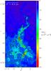 |
Fig. 1 N(H2) map of IRDC G11.11-0.12, derived using NIR and MIR dust extinction data. The spatial resolution of the map is 2″ and it covers the dynamic range of NH2 = 2−95 × 1021 cm-2. The contour levels are [3,10,15,25,...] × 1021 cm-2. The contour at 10 × 1021 cm-2 is bold. The coordinate system is tilted: the Galactic longitude is on y-axis and latitude on x-axis. |
3.1. Comparison of Herschel and dust extinction data
We first examined how the dust extinction- and Herschel-derived column densities compare by making a pixel-to-pixel comparison. For this analysis, the extinction data were smoothed to the  Herschel resolution. The comparison shows (Fig. 2, top frame) that the two column density measurement techniques are in a very good agreement. Note that the column densities (at this resolution) extend only to about N(H2) ≲ 70 × 1021 cm-2. Figure 2 (bottom frame) shows a histogram of the ratio of the two column density measurements. The histogram is shown separately for the entire mapped area (black curve) and for the area with N(H2) > 10 × 1021 cm-2. The histograms peak strongly at a ratio of unity. About 70% of all pixel values are within a factor of two from one-to-one relation. Above N(H2) > 10 × 1021 cm-2, the corresponding percentage is 90%. The full histogram has a tail toward higher ratios (i.e., Herschel data gives higher column densities) that can be attributed to a low-column density area N(H2) ≲ 5 × 1021 cm-2 in the north-west, part of the mapped region. It is possible that these discrepant values result, at least partly, from large-scale, systematic gradients in the emission detected from the diffuse Galactic dust component (our Herschel data analysis does not take such gradients into account). The histogram of the high-column density part does not show this discrepancy, indicating that if systematic background gradients are present, their effect is restricted to low-column density regions.
We conclude that the column densities derived from dust extinction and Herschel are in excellent agreement, given our current knowledge of dust opacities. As explained in Sect. 2.2, the dust opacities were chosen as a mean of plausible models, shown in Fig. A.1, which are nominally closest to the Ossenkopf & Henning (1994) model without dust coagulation. It is an interesting topic for future studies to examine whether this result holds in a larger sample of IRDCs. It could be hypothesized that dust coagulation may significantly alter dust opacities at the column densities our maps cover. However, as we will show in Sect. 3.3, the mean volume densities at the scale of the Herschel beam (~0.4 pc) are about 104 cm-3, not expected to be high enough for coagulation to be efficient (or, alternatively, would require relatively long time-scales, see, e.g., Ossenkopf & Henning 1994).
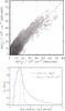 |
Fig. 2 Top: pixel-to-pixel comparison of column densities derived with the NIR+MIR dust extinction technique and the Herschel dust emission mapping. The color scale and contours show the density of data points in the scatter plot. The dashed line shows the one-to-one relation. The red solid line shows the median relationship. Bottom: histogram of the ratio of Herschel-derived column densities to NIR+MIR dust extinction derived column densities. The black solid line shows the histogram for all the data in the field. The blue line shows the histogram for the area with column density over N(H2) > 10 × 1021 cm-2. The dashed line shows the ratio of one. |
3.2. Column density distribution of G11
Figure 1 shows the N(H2) map of G11 derived from dust extinction. The total mass in the mapped area is Mtot ≈ 105 M⊙, regardless whether estimated from dust extinction or Herschel data. We estimate the mass associated with the filament-shaped part of the cloud from the column densities above N(H2) > 10 × 1021 cm-2, resulting in Mfil ≈ [1.3,2.5] × 104 M⊙. The lower limit is the mass after a subtraction of constant N(H2) = 10 × 1021 cm-2 from the filament area (to mimic a surrounding envelope), and the upper limit is the mass without subtraction. We find mean linear mass densities of Ml = [430,850] M⊙ pc-1 for the 30 pc long filament, i.e., on average Ml ≈ 600 M⊙ pc-1. The critical value for a self-gravitating, non-turbulent cylinder is 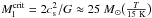 , where cs is the speed of sound (Ostriker 1964). In the case of turbulent support, the condition is
  pc-1 (Jackson et al. 2010). Assuming a typical value of ΔV = 2.5 km s-1 (see Sect. 3.3) results in Ml = 525 M⊙ pc-1. The linear mass density of G11 greatly exceeds the non-turbulent critical value and is approximately in agreement with the turbulent one. G11 clearly must be dominated by non-thermal motions.
We examined the distribution of mass in G11 by analyzing its dense gas mass fraction (DGMF, e.g., Lombardi et al. 2008; Kainulainen et al. 2009a; Kainulainen & Tan 2013), which describes the cumulative mass as a function of N(H2):  (3)where M( >N) is the mass above the column density N and Mtot the total mass. Figure 3 shows the DGMFs derived from both the dust extinction and Herschel data. They are very similar, except that the Herschel-derived DGMF stops at lower column densities because it averages column densities over larger area than the extinction data. The DGMFs are close-to exponentials above N(H2) ≳ 15 × 1021 cm-2 and have a slight deviation from it below that. An exponential fit, dM′ ∝ e− αN(H2), yields the slope of α = −0.07. This corresponds exactly to the mean DGMF derived for ten IRDCs by Kainulainen & Tan (2013) and shows that G11 is a typical high-mass IRDCs by its mass distribution.
We also compare the DGMFs of G11 to nearby, equally massive clouds Orion A and the California Cloud (Kainulainen et al. 2009a). Orion A is an active star-forming cloud, while the California Cloud is clearly more quiescent (Lada et al. 2009; Harvey et al. 2013). The DGMFs can depend on the resolution and dynamic range of the data. Therefore, we processed the N(H2) map of G11 to correspond to the data of Kainulainen et al. (2009a). We first truncated the G11 data to N(H2) < 25 × 1021 cm-2. Then, they were smoothed to 0.4 pc resolution. The resulting DGMF (Fig. 3) of G11 resembles that of Orion A.
Recently, Lada et al. (2012) suggested that the DGMF has a major role in setting the star formation efficiencies (SFEs) in molecular clouds throughout the entire mass scale of star formation. This picture was based on the observations that the DGMFs of nearby star-forming clouds are clearly flatter than those of quiescent clouds (Kainulainen et al. 2009a; Lada et al. 2010) and that star-forming rates of molecular clouds correlate better with the amount of dense gas in them than with their total masses (Lada et al. 2010). However, G11 (and other IRDCs) shows a relatively flat DGMF despite its arguably early stage of evolution and low SFE. This implies that the DGMF and SFE may not be as closely linked as earlier suggested. Indeed, in Kainulainen et al. (2013) we examined the physical parameters affecting the DGMFs in a sample of numerical turbulence simulations. We found that in addition to SFE, the average mixture of gas compression is an important (and in fact, the dominant) parameter in setting the observed DGMFs. The flat DGMF of G11 supports this picture: it appears that G11 has developed a large amount of dense gas despite its low SFE. One possible explanation for this is that the environment in which G11 resides is different from that of local clouds. This kind of galaxy-scale variations in the density statistics of molecular clouds has recently been found in the nearby M51 galaxy (Hughes et al. 2013). In M51, the spiral arm regions show higher relative amounts of dense gas than inter-arm regions. We hypothesize that the same phenomenon is seen when the DGMFs of nearby clouds are compared with G11.
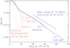 |
Fig. 3 DGMFs of G11, derived using NIRMIR dust extinction (blue) and Herschel (black). The red lines show the DGMFs of the California Cloud and Orion A (Kainulainen et al. 2009a), and of G11 with the same spatial resolution and column density range. The figure also shows a blue line indicating the slope of an exponential fit to the the mean DGMF of ten IRDCs from Kainulainen & Tan (2013). The fit was done to the DGMFs above N(H2) ≳ 7 × 1021 cm-2. |
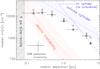 |
Fig. 4 Median mean densities ( |

3.3. Tracing multi-scale fragmentation in G11
The high-spatial resolution and sensitivity of the extinction data allows us to study fragmentation in G11 over wide ranges of sizes and densities. In general, describing the hierarchical structure of molecular clouds is non-trivial, and there are many tools available for the purpose (e.g., Stutzki et al. 1998; Alves et al. 2007; Burkhart et al. 2009). Here, we aim at an analysis that describes the scale-dependency of fragmentation in G11. We use a size-scale-based approach employed in Alves et al. (2007). It entails performing a wavelet-decomposition of the N(H2) data and identifying significant, single-peaked structures at different filtering scales of the decomposition. The approach is analogous to high-pass filtering, but also incorporates object recognition over multiple spatial scales. This makes the method less prone to detect spurious structures that are present in only one scale and do not correspond to real column density features (Kainulainen et al. 2009b). The algorithm results in identification of structures at scales that are {4,8,16,... } pixels in size, corresponding to {0.08,0.17,0.34,... } pc. For example, 128 significant structures are found at the smallest (0.08 pc) spatial scale.
We identified structures located within the large-scale filament, and calculated their median separations and mean densities. We used both spherical and cylindric approximations in calculating volume densities. Assuming spherical geometry gives  where M and A are the mass and area, and μ and mH the mean molecular weight and hydrogen mass. The cylindric geometry gives
  , where b and h are the minor axis of the structure and its length, respectively. The relationship of the resulting volume densities and separations is shown in Fig. 4. The figure also shows the predictions from the spherical Jeans’ instability and the analogy of it in infinitely long, cylindric case (e.g., Chandrasekhar & Fermi 1953; Inutsuka & Miyama 1992; Jackson et al. 2010). In the former model, the core separation is related to density via Jeans’ length,
  . In the latter model, the separation depends on the filament scale height H = cs(4πGρc)− 1/2 and radius R. When R ≫ H, the separation is λmax = 22H. In G11, the mean density at largest scales is
  cm-3 and H ≈ 0.17 pc, assuming T = 15 K. The radius of the large-scale filament is ~0.7 pc. Thus, it appears that we can estimate the separation scale with λmax = 22H (as in Jackson et al. 2010). However, this prediction is for non-turbulent case, while G11 should be mainly supported by non-thermal motions (cf., Sect. 3.2). While we do not have detailed velocity data for the purpose, we assume Larson’s relationship, σv = 720 m s-1(R/1 pc)0.5, as an estimate of line-widths in G11, which is in rough agreement with pointings in NH3 (Pillai et al. 2006b). The predicted separations are calculated by replacing the cs with σv and are shown in Fig. 4.
The fragmentation characteristics of G11 are in agreement with the predictions for a self-gravitating cylinder at scales l ≳ 0.5 pc. At smaller scales, the relationship between density and separation appears to change, and the observations are in better agreement with Jeans’ fragmentation. We hypothesize that at large scales, the fragmentation is driven by the global, filamentary nature of the cloud, while at smaller scales local fragmentation is insensitive to the large-scale geometry. We also consider that the finite nature of the G11 filament may play a role in the collapse time-scales in light of the recent predictions by Pon et al. (2011). They relate the local and global collapse time-scales by 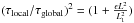 , where L and L1 are the global and local size-scales, respectively, and ϵ is the relative enhancement of mass line density that serves as the seed of the collapse. It follows that the time-scale of local collapse becomes much (more than ten times) shorter than global collapse at the size-scale of [0.2,2] pc, corresponding to choices of ϵ = [0.01,0.5]. While this range of scales is large, it shows that there indeed should be a size-scale at which the fragmentation becomes physically dominated by local instead of global processes. Our observations of G11 suggest that this size-scale is at about ~0.5 pc where we see a flattening in the density-separation relation.
The scale-dependency of fragmentation in G11 may relate to the velocity structure of the cloud. Recently, Hacar et al. (2013) showed that the 10 pc long B213 filament is built up by r ≳ 0.5 pc sized filament “bundles”. The bundles contain multiple velocity-coherent filaments that are further fragmented into cores. They propose that this hierarchy may originate from scale-dependent contraction time-scales. Our results for G11 fit well in this picture. The transition in fragmentation characteristics of G11 occurs at ~0.5 pc, which is the characteristic size of the velocity-coherent filaments identified by Hacar et al. (2013). One explanation is that at these scales the local collapse time becomes sufficiently short compared to the global collapse time, enabling small-scale fragmentation (to dense cores) unaffected by large-scale instabilities. We will investigate this further with kinematic data in a forthcoming paper (Ragan et al., in prep.).
4. Conclusions
We analyze the column density distribution of the high-mass, filamentary IRDC G11.11-0.12 (G11) using combined NIR+MIR dust extinction data and Herschel dust emission data. Our conclusions are as follows.
-
1.
The combined NIR+MIR dust extinction map reveals the column density structure of the G11 filament in a resolution of 2″ (0.035 pc) over the range of N(H2) ≈ 2 − 100 × 1021 cm-2. The column densities derived from the NIR+MIR data and Herschel data are in excellent agreement. The total mass of G11 is about 105 M⊙, from which ~2 × 10⁴ M⊙ is associated with the 30 pc long filamentary structure.
-
2.
The dense gas mass fraction (DGMF) of G11 is typical for high-mass IRDCs, showing that it harbors a relatively large amount of dense gas, comparable to active nearby star-forming clouds, e.g., Orion A. The linear mass density of the large-scale filament in G11 is high, Ml ≈ 600 M⊙ pc-1, also similar to the Orion filament (Ml ~ 325 M⊙ pc-1). However, the star-forming activity of G11 is arguably much lower than that of the Orion filament. This suggests that the amount of dense gas in molecular clouds is not directly connected to their star-forming efficiencies (cf., Lada et al. 2010), but is rather set by other parameters/processes, possibly prior to the most active star-forming phase of the clouds. One explanation that can account for this is the average level of gas compression in molecular clouds (cf., Kainulainen et al. 2013) that depends on the galaxy-scale environment. This picture is supported by the environment-dependence of the molecular clouds’ density statistics in M51 (e.g., Hughes et al. 2013).
-
3.
We find that the structure of G11 is in agreement with hierarchical fragmentation of a self-gravitating cylinder at sizes larger than r ≳ 0.5 pc. At smaller scales, the fragmentation more closely resembles Jeans’ fragmentation. This suggests that the fragmentation at large scales is dominated by the collapse of the natal filament, while at small-scales the filamentary origin does not play a role, but fragmentation depends on local properties only. This hypothesis is in agreement with scale-dependent collapse time-scales derived for finite filaments (Pon et al. 2011).
Acknowledgments
The authors are grateful to Fabian Heitsch, Henrik Beuther, and Alvaro Hacar for helpful discussions, and to Anika Schmiedeke for her role in the reduction of the Herschel data used in this work. The work of J.K., S.R., and A.S. was supported by the Deutsche Forschungsgemeinschaft priority program 1573 (“Physics of the Interstellar Medium”).
References
- Alves, J., Lombardi, M., & Lada, C. J. 2007, A&A, 462, L17 [NASA ADS] [CrossRef] [EDP Sciences] [Google Scholar]
- André, P., Men’shchikov, A., Bontemps, S., et al. 2010, A&A, 518, L102 [NASA ADS] [CrossRef] [EDP Sciences] [Google Scholar]
- Benjamin, R. A., Churchwell, E., Babler, B. L., et al. 2003, PASP, 115, 953 [NASA ADS] [CrossRef] [Google Scholar]
- Beuther, H., Henning, T., Linz, H., et al. 2010, A&A, 518, L78 [NASA ADS] [CrossRef] [EDP Sciences] [Google Scholar]
- Bohlin, R. C., Savage, B. D., & Drake, J. F. 1978, ApJ, 224, 132 [NASA ADS] [CrossRef] [Google Scholar]
- Burkhart, B., Falceta-Gonçalves, D., Kowal, G., & Lazarian, A. 2009, ApJ, 693, 250 [NASA ADS] [CrossRef] [Google Scholar]
- Cardelli, J. A., Clayton, G. C., & Mathis, J. S. 1989, ApJ, 345, 245 [NASA ADS] [CrossRef] [Google Scholar]
- Carey, S. J., Feldman, P. A., Redman, R. O., et al. 2000, ApJ, 543, L157 [NASA ADS] [CrossRef] [Google Scholar]
- Chandrasekhar, S., & Fermi, E. 1953, ApJ, 118, 116 [NASA ADS] [CrossRef] [MathSciNet] [Google Scholar]
- Hacar, A., Tafalla, M., Kauffmann, J., & Kovacs, A. 2013, A&A, 554, A55 [NASA ADS] [CrossRef] [EDP Sciences] [Google Scholar]
- Harvey, P. M., Fallscheer, C., Ginsburg, A., et al. 2013, ApJ, 764, 133 [NASA ADS] [CrossRef] [Google Scholar]
- Hennebelle, P., & Falgarone, E. 2012, A&ARv, 20, 55 [NASA ADS] [CrossRef] [Google Scholar]
- Henning, T., Linz, H., Krause, O., et al. 2010, A&A, 518, L95 [NASA ADS] [CrossRef] [EDP Sciences] [Google Scholar]
- Hughes, A., Meidt, S. E., Schinnerer, E., et al. 2013, ApJ, accepted [arXiv:1304.1219] [Google Scholar]
- Inutsuka, S.-I., & Miyama, S. M. 1992, ApJ, 388, 392 [NASA ADS] [CrossRef] [Google Scholar]
- Jackson, J. M., Finn, S. C., Chambers, E. T., et al. 2010, ApJ, 719, L185 [NASA ADS] [CrossRef] [Google Scholar]
- Johnstone, D., Fiege, J. D., Redman, et al. 2003, ApJ, 588, L37 [NASA ADS] [CrossRef] [Google Scholar]
- Kainulainen, J., & Tan, J. C. 2013, A&A, 549, A53 [NASA ADS] [CrossRef] [EDP Sciences] [Google Scholar]
- Kainulainen, J., Beuther, H., Henning, T., & Plume, R. 2009a, A&A, 508, L35 [NASA ADS] [CrossRef] [EDP Sciences] [Google Scholar]
- Kainulainen, J., Lada, C. J., Rathborne, J. M., & Alves, J. F. 2009b, A&A, 497, 399 [NASA ADS] [CrossRef] [EDP Sciences] [Google Scholar]
- Kainulainen, J., Alves, J., Beuther, H., et al. 2011, A&A, 536, A48 [NASA ADS] [CrossRef] [EDP Sciences] [Google Scholar]
- Kainulainen, J., Federrath, C., & Henning, T. 2013, A&A, 553, L8 [Google Scholar]
- Lada, C. J., Lombardi, M., & Alves, J. F. 2009, ApJ, 703, 52 [NASA ADS] [CrossRef] [Google Scholar]
- Lada, C. J., Lombardi, M., & Alves, J. F. 2010, ApJ, 724, 687 [NASA ADS] [CrossRef] [Google Scholar]
- Lada, C. J., Forbrich, J., Lombardi, M., & Alves, J. F. 2012, ApJ, 745, 190 [NASA ADS] [CrossRef] [Google Scholar]
- Launhardt, R., Stutz, A. M., Schmiedeke, A., et al. 2013, A&A, 551, A98 [NASA ADS] [CrossRef] [EDP Sciences] [Google Scholar]
- Lawrence, A., Warren, S. J., Almaini, O., et al. 2007, MNRAS, 379, 1599 [NASA ADS] [CrossRef] [MathSciNet] [Google Scholar]
- Lombardi, M., Lada, C. J., & Alves, J. 2008, A&A, 489, 143 [NASA ADS] [CrossRef] [EDP Sciences] [Google Scholar]
- Marshall, D. J., Robin, A. C., Reylé, C., et al., 2006, A&A, 453, 635 [NASA ADS] [CrossRef] [EDP Sciences] [Google Scholar]
- Ossenkopf, V., & Henning, T. 1994, A&A, 291, 943 [NASA ADS] [Google Scholar]
- Ostriker, J. 1964, ApJ, 140, 1056 [NASA ADS] [CrossRef] [MathSciNet] [Google Scholar]
- Ott, S. 2010, in Astronomical Data Analysis Software and Systems XIX, eds. Y. Mizumoto, K.-I. Morita, & M. Ohishi, ASP Conf. Ser., 434, 139 [Google Scholar]
- Peretto, N., & Fuller, G. A. 2009, A&A, 505, 405 [NASA ADS] [CrossRef] [EDP Sciences] [Google Scholar]
- Pilbratt, G. L., Riedinger, J. R., Passvogel, T., et al. 2010, A&A, 518, L1 [CrossRef] [EDP Sciences] [Google Scholar]
- Pillai, T., Wyrowski, F., Menten, K. M., & Krügel, E. 2006a, A&A, 447, 929 [NASA ADS] [CrossRef] [EDP Sciences] [Google Scholar]
- Pillai, T., Wyrowski, F., Carey, S. J., & Menten, K. M. 2006b, A&A, 450, 569 [NASA ADS] [CrossRef] [EDP Sciences] [Google Scholar]
- Pon, A., Johnstone, D., & Heitsch, F. 2011, ApJ, 740, 88 [NASA ADS] [CrossRef] [Google Scholar]
- Ragan, S. E., Bergin, E. A., & Gutermuth, R. A. 2009, ApJ, 698, 324 [NASA ADS] [CrossRef] [Google Scholar]
- Ragan, S., Henning, T., Krause, O., et al. 2012, A&A, 547, A49 [NASA ADS] [CrossRef] [EDP Sciences] [Google Scholar]
- Roussel, H. 2012 [arXiv:1205.2576] [Google Scholar]
- Savage, B. D., Bohlin, R. C., Drake, J. F., & Budich, W. 1977, ApJ, 216, 291 [NASA ADS] [CrossRef] [Google Scholar]
- Schneider, N., Csengeri, T., Hennemann, M., et al. 2012, A&A, 540, L11 [NASA ADS] [CrossRef] [EDP Sciences] [Google Scholar]
- Schuller, F., Menten, K. M., Contreras, Y., et al. 2009, A&A, 504, 415 [NASA ADS] [CrossRef] [EDP Sciences] [Google Scholar]
- Stanke, T., Smith, M. D., Gredel, R., & Khanzadyan, T. 2006, A&A, 447, 609 [NASA ADS] [CrossRef] [EDP Sciences] [Google Scholar]
- Stutzki, J., Bensch, F., Heithausen, A., et al. 1998, A&A, 336, 697 [NASA ADS] [Google Scholar]
- Weingartner, J. C., & Draine, B. T. 2001, ApJ, 548, 296 [NASA ADS] [CrossRef] [Google Scholar]
Appendix A: Comparison of dust extinction and Herschel-derived column densities
Appendix A.1: Dust opacity law
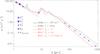 |
Fig. A.1 Dust opacity-law adopted for the work. The five lines show different plausible dust opacity models from Ossenkopf & Henning (1994) and Weingartner & Draine (2001). The symbols show the adopted dust opacities in NIR and 8 μm (cf., Kainulainen & Tan 2013) and in Herschel wavebands. The adopted values represent the mean values in the range set by the five shown models. |
Figure A.1 shows the absolute dust opacity law adopted in transforming NIR+MIR optical depths and sub-mm dust emission data to column densities. The figure shows five plausible dust opacity models. These were the Ossenkopf & Henning (1994) models with moderate dust coagulation and without dust coagulation, and Weingartner & Draine (2001) models with different RV values. The effective dust opacities used in NIR and 8 μm are close to the mean values of these models. Therefore, we chose in this work to use a corresponding definition to set the sub-mm opacities. The chosen values are shown in the figure and they are nominally closest to the Ossenkopf & Henning (1994) model without dust coagulation.
Appendix A.2: Effect of variable background to the Herschel-derived temperatures and column densities
We performed a Monte Carlo simulation to examine the effects of variable background emission to the column densities derived using Herschel dust emission data and the fitting technique described by Launhardt et al. (2013). Figure A.2 summarizes the results. The results are presented and discussed in Sect. 3.1.
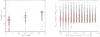 |
Fig. A.2 Effect of the variable background emission to the Herschel-derived temperatures and column densities. The panels show results of a Monte Carlo simulation, in which normally-distributed random variations were imposed on a large sample model SEDs. Left: the output temperature for three values of input temperatures, {15,20,25} K. The repetitions of the simulation are shown with light-grey circles. The red boxes indicate inter-quartile ranges, with a horizontal line at the mean value, and the whiskers show ranges that extend to 1.5 times the inter-quartile range. Right: the same for the ratio of input to output column densities as a function of input column density. The blue dashed line shows the standard deviation, which is approximately 30% irrespective of the original column density. |
All Figures
|
Fig. 1 N(H2) map of IRDC G11.11-0.12, derived using NIR and MIR dust extinction data. The spatial resolution of the map is 2″ and it covers the dynamic range of NH2 = 2−95 × 1021 cm-2. The contour levels are [3,10,15,25,...] × 1021 cm-2. The contour at 10 × 1021 cm-2 is bold. The coordinate system is tilted: the Galactic longitude is on y-axis and latitude on x-axis. |
| In the text | |
|
Fig. 2 Top: pixel-to-pixel comparison of column densities derived with the NIR+MIR dust extinction technique and the Herschel dust emission mapping. The color scale and contours show the density of data points in the scatter plot. The dashed line shows the one-to-one relation. The red solid line shows the median relationship. Bottom: histogram of the ratio of Herschel-derived column densities to NIR+MIR dust extinction derived column densities. The black solid line shows the histogram for all the data in the field. The blue line shows the histogram for the area with column density over N(H2) > 10 × 1021 cm-2. The dashed line shows the ratio of one. |
| In the text | |
|
Fig. 3 DGMFs of G11, derived using NIRMIR dust extinction (blue) and Herschel (black). The red lines show the DGMFs of the California Cloud and Orion A (Kainulainen et al. 2009a), and of G11 with the same spatial resolution and column density range. The figure also shows a blue line indicating the slope of an exponential fit to the the mean DGMF of ten IRDCs from Kainulainen & Tan (2013). The fit was done to the DGMFs above N(H2) ≳ 7 × 1021 cm-2. |
| In the text | |
|
Fig. 4 Median mean densities ( |
| In the text | |
|
Fig. A.1 Dust opacity-law adopted for the work. The five lines show different plausible dust opacity models from Ossenkopf & Henning (1994) and Weingartner & Draine (2001). The symbols show the adopted dust opacities in NIR and 8 μm (cf., Kainulainen & Tan 2013) and in Herschel wavebands. The adopted values represent the mean values in the range set by the five shown models. |
| In the text | |
|
Fig. A.2 Effect of the variable background emission to the Herschel-derived temperatures and column densities. The panels show results of a Monte Carlo simulation, in which normally-distributed random variations were imposed on a large sample model SEDs. Left: the output temperature for three values of input temperatures, {15,20,25} K. The repetitions of the simulation are shown with light-grey circles. The red boxes indicate inter-quartile ranges, with a horizontal line at the mean value, and the whiskers show ranges that extend to 1.5 times the inter-quartile range. Right: the same for the ratio of input to output column densities as a function of input column density. The blue dashed line shows the standard deviation, which is approximately 30% irrespective of the original column density. |
| In the text | |
Current usage metrics show cumulative count of Article Views (full-text article views including HTML views, PDF and ePub downloads, according to the available data) and Abstracts Views on Vision4Press platform.
Data correspond to usage on the plateform after 2015. The current usage metrics is available 48-96 hours after online publication and is updated daily on week days.
Initial download of the metrics may take a while.