| Issue |
A&A
Volume 556, August 2013
|
|
|---|---|---|
| Article Number | A56 | |
| Number of page(s) | 11 | |
| Section | Stellar structure and evolution | |
| DOI | https://doi.org/10.1051/0004-6361/201321702 | |
| Published online | 25 July 2013 | |
KIC 11285625: A double-lined spectroscopic binary with a γ Doradus pulsator discovered from Kepler space photometry ⋆,⋆⋆
1 Instituut voor Sterrenkunde, KU Leuven, Celestijnenlaan 200B, 3001 Leuven, Belgium
e-mail: jonas@ster.kuleuven.be
2 Department of Astrophysics, Radboud University Nijmegen, PO Box 9010, 6500 GL Nijmegen, The Netherlands
3 Department of Physics, Faculty of Science, University of Zagreb, Croatia
4 INAF – Osservatorio Astronomico di Roma via Frascati 33, 00040 Monteporzio C. (RM), Italy
5 Jeremiah Horrocks Institute, University of Central Lancashire, Preston PR1 2HE, UK
6 Astrophysics Group, Keele University, Staffordshire ST5 5BG, UK
7 Stellar Astrophysics Center, Department of Physics and Astronomy, Aarhus University, Ny Munkegade 120, 8000 Aarhus C, Denmark
Received: 15 April 2013
Accepted: 30 May 2013
Aims. We present the first binary modelling results for the pulsating, eclipsing binary KIC 11285625 that was discovered by the Kepler mission. An automated method to disentangle the pulsation spectrum and the orbital variability in high quality light curves was developed and applied. The goal was to obtain accurate orbital and component properties in combination with essential information derived from spectroscopy.
Methods. A binary model for KIC 11285625 was obtained, using a combined analysis of high-quality space-based Kepler light curves and ground-based high-resolution HERMES echelle spectra. The binary model was used to separate the pulsation characteristics from the orbital variability in the Kepler light curve in an iterative way. We used an automated procedure based on the JKTEBOP binary modelling code to perform this task, and adapted codes for frequency analysis and prewhitening of periodic signals. Using a disentangling technique applied to the composite HERMES spectra, we obtained a higher signal-to-noise mean spectrum for both the primary and the secondary components. A model grid search method for fitting synthetic spectra was used for fundamental parameter determination for both components.
Results. Accurate orbital and component properties of KIC 11285625 were derived, and we have obtained the pulsation spectrum of the γ Dor pulsator in the system. Detailed analysis of the pulsation spectrum revealed amplitude modulation on a timescale of a hundred days, and strong indications of frequency splittings at both the orbital frequency and the rotational frequency derived from spectroscopy.
Key words: stars: oscillations / binaries: spectroscopic / techniques: photometric / stars: rotation / stars: fundamental parameters / binaries: eclipsing
Partly based on observations made with the Mercator Telescope, which is operated on the island of La Palma by the Flemish Community, at the Spanish Observatorio del Roque de los Muchachos of the Instituto de Astrofisica de Canarias. Based on observations obtained with the HERMES spectrograph, which is supported by the Fund for Scientific Research of Flanders (FWO), Belgium, the Research Council of K.U. Leuven, Belgium, the Fonds National Recherches Scientific (FNRS), Belgium, the Royal Observatory of Belgium, the Observatoire de Genève, Switzerland, and the Thüringer Landessternwarte Tautenburg, Germany.
Full Table 5 is available at the CDS via anonymous ftp to cdsarc.u-strasbg.fr (130.79.128.5) or via http://cdsarc.u-strasbg.fr/viz-bin/qcat?J/A+A/556/A56
© ESO, 2013
1. Introduction
NASA’s Kepler mission has been continuously monitoring more than 150 000 stars for the past four years, searching for transiting exoplanets (Borucki et al. 2010). The unprecedented quality of the photometric light curves delivered by Kepler makes them very well suited to study stellar variability in general. Automated light curve classification techniques with the goal to recognize and identify the many variable stars hidden in the Kepler database have been developed. The application of these methods to the public Kepler Q1 data is described in Debosscher et al. (2011). The authors paid special attention to the detection of pulsating stars in eclipsing binary systems there. These systems are relatively rare and especially interesting for asteroseismic studies (see e.g. Maceroni et al. 2009; Welsh et al. 2011). By modelling the orbital dynamics of the binary using photometric time series that are complemented with spectroscopic follow-up observations, we can obtain accurate constraints on the masses and radii of the pulsating stars. These constraints are needed for asteroseismic modelling and are difficult to obtain otherwise.
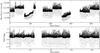 |
Fig. 1 Combination of observing quarters Q1-Q10 for KIC 11285625. The top panel shows the raw SAP (simple aperture photometry) fluxes, as they were delivered, while the lower panel shows the resulting combined dataset after optimal mask selection and detrending. |
Numerous candidate pulsating binaries were identified in the Kepler data, and spectroscopic follow-up is ongoing. In this work, we present the results obtained for KIC 11285625 (BD+48 2812), which turns out to be an eclipsing binary system containing a γ Dor pulsators. The Kepler Input Catalog (KIC) lists the following properties for this target: V = 10.143 mag, Teff = 6882 K, log g = 3.753, R = 2.61 R⊙, and [Fe/H] = −0.127. Spectroscopic follow-up revealed it to be a double-lined binary (Sect. 3). Currently, only a few γ Dor pulsators in double-lined spectroscopic binaries are known, making their analysis very relevant for asteroseismology. Maceroni et al. (2013) studied a γ Dor pulsator in an eccentric binary system, observed by CoRoT. Here, we are dealing with a non-eccentric system with a longer orbital period. The longer time span and the higher photometric precision of the Kepler obse rvations (almost a factor 6) allowed us to study the pulsation spectrum with a significantly increased frequency resolution and lower amplitudes.
A combined analysis of the Kepler light curve and spectroscopic radial velocities (RV) allowed us to obtain a good binary model for KIC 11285625, resulting in accurate estimates of the masses and radii of both components (Sect. 4). This binary model was also used to disentangle the pulsations from the orbital variability in the Kepler light curve in an iterative way. In this paper, we describe procedures to perform this task in an automated way. The low signal-to-noise composite spectra used for the determination of the RVs were used to obtain higher signal-to-noise mean spectra of the components by means of spectral disentangling. These spectra were then used to obtain fundamental parameters of the stars (Sect. 5). The resulting pulsation signal of the primary is analysed in detail in Sect. 6. We discuss there the global characteristics of the frequency spectrum, list the dominant frequencies and their amplitudes detected by means of prewhitening, and search for signs of rotational splitting.
 |
Fig. 2 Kepler aperture (left) and a single target pixel image (right) for KIC 11285625 at quarter Q3. Red colours in the pixel image indicate the lowest flux levels, white colours indicate the highest flux levels. |
2. Kepler data
KIC 11285625 has been almost continuously observed by Kepler; data are available for the observing quarters Q0-Q10. We used only long cadence data in this work (with a time resolution of 29.4 min), since short cadence data are only available for three quarters and are not needed for our purposes. During quarter Q4, one of the CCD modules failed, the reason why part of the Q4 data are missing. No Q8 data could be observed either, since the target was positioned on the same broken CCD module during that quarter. The Kepler spacecraft needs to make rolls every three months (for continuous illumination of its solar arrays), causing targets to fall on different CCD modules depending on the observing quarter. Given the different nature of the CCDs and the different aperture masks used, this caused some issues with the data reduction. The average flux level of the light curve for KIC 11285625 varies significantly between quarters, and for some, instrumental trends are visible. The top panel of Fig. 1 plots all the observed datasets, showing the quarter-to-quarter variations. Merging the quarters correctly is not trivial, since the trends have to be removed for each quarter separately, and the data have to be shifted so that all quarters are at the same average level (see below). Often, polynomials are used to remove the trends, but it is difficult to determine a reasonable order for the polynomial. This is especially the case when large amplitude variability is present in the light curve, at timescales comparable to the total time span of the data.
Fortunately, pixel target files are available for all observed quarters for KIC 11285625, allowing us to do the light curve extraction based on custom aperture masks. We can define a custom aperture mask, determining which pixels to include or not. It turns out that the standard aperture mask used by the data reduction pipeline was not optimal for all quarters. This is clearly visible in the top panel of Fig. 1 for quarters Q3 and Q7. The clear upward trends and smaller variability amplitudes, compared to the other quarters, are caused by a suboptimal aperture mask. The trends can be explained by a small drift of the star on the CCD, changing the amount of stellar flux included in the aperture during the quarter. Checking the target pixel files for those quarters revealed that pixels with significant flux contribution were not included in the mask. Figure 2 shows the Kepler aperture from the automated pipeline and a single target pixel image obtained during quarter Q3. As can be seen, the Kepler aperture misses a pixel with significant flux contribution (the lowest blue coloured pixel). Adding this pixel to the aperture mask effectively removed the trend in the light curve and increased the variability amplitude to the level of the other quarters.
An automated method was developed to optimize the aperture mask for each quarter with the goal to maximize the signal-to-noise ratio (S/N) in the Fourier amplitude spectrum. The standard mask provided with the target pixel files is used as a starting point. The method then loops over each pixel in the images outside of the original mask delivered by the Kepler pipeline. For each of those pixels, a new light curve is constructed by adding the flux values of the pixel to the summed flux of the pixels within the original Kepler mask. The amplitude spectrum of the resulting light curve is then computed, and the S/N of the highest peak (in this case, the main pulsation frequency of the star) is determined. If the addition of the pixel increases the S/N (by a user specified amount), it will be added to the final new light curve once each pixel has been analysed this way. The method also avoids adding pixels containing significant flux of neighbouring contaminating targets, since these will normally decrease the S/N of the signal coming from the main target. It is also possible to detect contaminating pixels within the original Kepler mask using exactly the same method, however we now exclude one pixel at a time from the original mask and check the resulting S/N of the new light curves.
After determining a new optimal aperture mask for each quarter, the resulting light curves still showed some small trends and offsets, but they were easily corrected using second order polynomials. Special care is needed however when shifting quarters to the same level, since the average value of the light curve might be ill determined, especially when large amplitude non-sinusoidal variability is present at timescales similar to the duration of an observing quarter. In our case, we want to make the average out-of-eclipse brightness match between different quarters and not the global average of the quarters, since the latter is shifted due to the presence of the eclipses. Therefore, we first cut out the eclipses and interpolated the data points in the resulting gaps using cubic splines. This was done only to determine the polynomial coefficients, which were then used to subtract the trends from the original light curves (including the eclipses). We first transformed the fluxes into magnitudes for each quarter separately, prior to trend removal. The binary modelling code described further needs magnitudes as input, but the conversion to magnitude also resolves any potential quarter-to-quarter variability amplitude changes that are caused by e.g., a difference in CCD gains (or any other instrumental effect changing the flux values in a linear way). The lower panel of Fig. 1 shows the resulting light curve after application of our detrending procedure using target pixel files.
3. Spectroscopic follow-up and RV determination
Spectroscopic follow-up observations were obtained with the HERMES Echelle spectrograph at the Mercator telescope on La Palma (see Raskin et al. 2011 for a detailed description of the instrument). In total, 63 spectra with good orbital phase coverage were observed with S/N in V in the range 40–70. These spectra revealed the double-lined nature of the spectroscopic binary.
RVs were derived with the HERMES reduction pipeline, using the cross-correlation technique with an F0 spectral mask. The choice for this mask was based on the F0 spectral type given by SIMBAD and the effective temperature listed in the KIC. We also tried additional spectral masks, given the double-lined nature of the binary, but we did not obtain better results in terms of scatter on the RV points. Due to the numerous metal lines in the spectrum, the cross-correlation technique worked very well, despite the relatively low S/N spectra. The upper panel of Fig. 3 shows the RV measurements obtained for both components of KIC 11285625. The black circles correspond to the primary component and the red circles to the secondary component. From the scatter on the RV measurements, we conclude that the primary component is pulsating. A Keplerian model was fitted for both components (shown also in the upper panel of Fig. 3 ), resulting in the orbital parameters listed in Table 1.
Uncertainties were estimated using a Monte-Carlo perturbation approach. Although the orbital period of the system can be a free parameter in the fitting procedure for the Keplerian model, we fixed it to the much more accurate value obtained from the Kepler light curve, given its longer time span (see Sect. 4). The quality of the fit obtained this way (as judged from the χ2 values) is significantly better compared to the case where the orbital period is left as a free parameter.
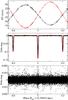 |
Fig. 3 Upper panel: phased HERMES RV data (open circles) and Keplerian model fits (lines) for both components (black: primary, red: secondary). Middle panel: phased Kepler data (pulsations removed) with the binary model overplotted in red. Lower panel: phased residuals of the Kepler data after removal of both the pulsations and the binary model. |
4. Binary model
We used the combined Kepler Q1–Q10 data to obtain a binary model, which provided us with accurate estimates of the main astrophysical properties of both components when combined with the results from the spectroscopic analysis. Given that we are dealing with a detached binary with no or only limited distortion of both components, we used JKTEBOP, which is written by J. Southworth (see Southworth et al. 2004a,b). This code is based on the EBOP code, originally developed by Paul B. Etzel (see Etzel 1981; Popper & Etzel 1981). JKTEBOP has the advantage of being very stable, fast, and applicable to large datasets with thousands of measurements, such as the Kepler light curves. Moreover, it can easily be scripted (essential in our approach) and includes useful error analysis options, such as Monte Carlo and bootstrapping methods.
Since we are dealing with a light curve containing both orbital variability (eclipses) and pulsations, we had to disentangle both phenomena to obtain a reliable binary model. In the amplitude spectrum of the Kepler light curve (see Fig. 4), the γ Dor type pulsations have numerous significant peaks in the range 0−0.7 d-1 with clear repeating patterns up to around 4 d-1. In the same region of the amplitude spectrum, we also find peaks corresponding to the orbital variability: a comb-like pattern of harmonics of the orbital frequency (forb, 2forb, 3forb,...). Moreover, the main pulsation frequency of 0.567 d-1 is close to 6forb (0.556 d-1), though the peaks are clearly separated, at a given estimated frequency resolution of 1/T ≈ 0.0012 d-1, where T is the total time span of the combined Kepler Q1–Q10 data. This near coincidence complicated the disentangling of both types of variability in the light curve, unlike the case where the orbital variability is well separated from the pulsations in the frequency domain (e.g., typical for a δ Sct pulsator in a long-period binary). We used an iterative procedure consisting of an alternation of binary modelling with JKTEBOP and of prewhitening of the remaining variability (pulsations) after removal of the binary model. This procedure can be done in an automated way, and the number of iterations can be chosen. The idea is that we gradually improve both the binary model and the residual pulsation spectrum at the same time. In each step of the procedure, we used the entire Q1–Q10 dataset without any rebinning. Our iterative method is similar to the one described in Maceroni et al. (2013) and consists of the following steps:
-
1.
Remove the eclipses from the original Kepler light curve andinterpolate the resulting gaps using cubic splines.
-
2.
Derive a first estimate of the pulsation spectrum by means of iterative prewhitening of the light curve without eclipses.
-
3.
Remove the pulsation model derived in the previous step from the original Kepler light curve.
-
4.
Find the best fitting binary model to the residuals using JKTEBOP.
-
5.
Remove this binary model from the original Kepler light curve (dividing by the model when working in flux or subtracting the model when working in magnitudes).
-
6.
Perform frequency analysis on the residuals, which delivers a new estimate of the pulsation spectrum.
-
7.
Subtract the pulsation model obtained in the previous step from the original Kepler light curve.
-
8.
Model the residuals (an improved estimate of the orbital variability) with JKTEBOP, and repeat the procedure starting from step five.
The procedure is then stopped when convergence is obtained: the χ2 value of the binary model no longer decreases significantly. In practice, convergence is obtained after just a few iterations, at least for KIC 11285625. The procedure can be run automatically, provided that the user has a good initial guess for the orbital parameters. The computation time is dominated by the prewhitening step, which requires the repeated calculation of amplitude spectra. In our case, the complete procedure required a few hours on a single desktop CPU. The top panel of Fig. 4 shows part of the original Kepler data with the disentangled pulsation contribution overplotted in red, the lower panel shows the corresponding amplitude spectrum. In Fig. 3, the Keplerian model fit to the HERMES RV data, the binary model fit to the Kepler data (pulsation part removed), and the residual light curve are shown together, and are phased with the orbital period (using the zero-point T0 = 2 454 953.751335 d, corresponding to a time of minimum of the primary eclipse). The slightly larger scatter in the residuals at the ingress and egress of the primary eclipse is caused by the occulted surface of the pulsating primary, which is non-uniform and changing over time due to the non-radial pulsations.
Orbital and physical parameters for both components of KIC 11285625 obtained from the combined spectroscopic and photometric analysis.
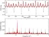 |
Fig. 4 Upper panel: resulting light curve after iterative removal of the orbital variability (in red) with the original light curve shown for comparison (in black). Lower panel: amplitude spectrum of the original Kepler light curve (in black) and the amplitude spectrum of the pulsation “residuals” (in red) after iterative removal of the orbital variability. |
We also investigated a different iterative approach, where we started by fitting a binary model directly to the original Kepler light curve instead of first removing the pulsations. In this way, we do not remove information from the light curve by cutting the eclipses, and we do not need to interpolate the data. Although the iterative procedure also converged quickly using this approach, the final binary model was not accurate. Removing the model from the original Kepler light curve introduced systematic offsets during the eclipses. The reason is that the initial binary model obtained from the original light curve is inaccurate due to the large amplitude and non-sinusoidal nature of the pulsations, causing the mean light level between eclipses to be badly defined. The approach starting from the light curve with the pulsations removed prior to binary modelling provided much better results, as judged from the χ2 values and visual inspection of the residuals during the eclipses.
A linear limb-darkening law was used for both stars with coefficients obtained from Prša et al. (2011)1. These coefficients have been computed for a grid of Teff, log g, and [M/H] values, considering Kepler’s transmission, CCD quantum efficiency, and optics. We estimated them using the KIC parameters for a first iteration but later adjusted them using our obtained values for Teff, log g, and [M/H] from the combination of binary modelling and spectroscopic analysis (see Sect. 5). We did not consider gravity darkening and reflection effects, given that both components are well separated, and are not significantly deformed by rapid rotation or binarity (the oblateness values returned by JKTEBOP are very small).
During the iterative procedure, special care was paid to the following issues, since they all influence the quality of the final binary and pulsation models:
-
Removal of the pulsations from the original light curve: Here, wefirst determined all the significant pulsation frequencies (or,more general: frequencies most likely not caused by the orbitalmotion) from the light curve with the eclipses removed. Onlyfrequencies with an amplitude S/N above four are considered.The noise level in the amplitude spectrum is determined from theregion 20–24 d-1, where no significant peaks are present. The often used procedure of computing the noise level in a region around the peak of interest would not provide reliable S/N estimates in our case, given the high density of significant peaks at low frequencies. We also used false-alarm probabilities as an additional significance test with very similar results regarding the number of significant frequencies.
-
Initial parameters of the binary model: when running JKTEBOP, initial parameters have to be provided for the binary model. These are then refined using non-linear optimization techniques (e.g. Levenberg-Marquardt). Although the optimization procedure is stable and converges fast, we have no guarantee that the global best solution is obtained. If the initial parameters are too far off from their true values, the procedure can end up in a local minimum. Therefore, we did some exploratory analysis first to find a good set of initial parameters, aided by the constraints obtained from the RV data. The initial parameters were also refined: After completion of the first iterative procedure, the final parameters were used as initial values for a new run, etc. This also confirmed the stability of the solution, although it does not guarantee that the overall best solution has been found.
Error analysis of the final binary model was done using the Monte-Carlo method implemented in JKTEBOP. Here, the input light curve (with the pulsations removed) is perturbed by adding Gaussian noise with a standard deviation estimated from the residuals, and the binary model is recomputed. This procedure is repeated typically 10 000 times to obtain confidence intervals for the obtained parameter values. The final parameters from the combined spectroscopic and photometric analysis and their estimated uncertainties (1σ) are listed in Table 1.
Given the long time span and excellent time sampling of the light curve, we also checked for the presence of eclipse time variations (e.g., due to the presence of a third body). We used two different methods to check for deviations of pure periodicity of the eclipse times. The first method consists of computing the amplitude spectrum of each observing quarter of the light curve separately and of comparing the peaks caused by the binary signal (the comb of harmonics of the orbital frequency). We could not detect any change in orbital frequency this way. Moreover, the orbital peaks in the amplitude spectrum of the entire light curve also do not show any broadening or significant sidelobes (indicative of frequency changes), compared to the amplitude spectrum of the purely periodic light curve of our best binary model computed with JKTEBOP. The second method consists of determining the times of minima for each eclipse individually by fitting a parabola to the bottom of each eclipse and determining the minimum. We then compared those times with the predicted values using our best value of the orbital period (O–C diagram). This was done both for the original light curve and the light curve with pulsations removed. In the first case, we found indications of periodic shifts of the eclipse times, but these are clearly linked to the pulsation signal in the light curve, which also affects the eclipses. No periodic shifts or trends could be found when analysing the light curve with pulsations removed, and we conclude that we do not detect eclipse time variations.
5. Spectral disentangling
To derive the fundamental parameters Teff, log g, [M/H], etc. of the γ Dor pulsator from the high resolution HERMES spectra, we first needed to separate the contributions of both stars in the measured composite spectra. Given the similar spectral types of the components and the large number of metal lines in the spectra, we could apply the technique of spectral disentangling to accomplish this (Simon & Sturm 1994; Hadrava 1995). Here, we used the FDBinary code2, (Ilijic et al. 2004) which is based on Hadrava’s Fourier approach (Hadrava 1995). The overall procedures used to determine the orbital parameters and to reconstruct the spectra of the component stars from the time series of observed composite spectra of a spectroscopic double-lined eclipsing binary have been described extensively in Hensberge et al. (2000) and Pavlovski & Hensberge (2005).
The user has to provide good initial guesses and confidence intervals for the orbital parameters, otherwise the method might not converge towards the correct solution. Luckily, we had very good initial parameter values available from the Keplerian orbital fit to the RV data, as was described in Sect. 3. The final orbital parameters are in excellent agreement with the initial values derived from spectroscopy.
Spectral disentangling methods have the advantage that they enable us to determine the orbital parameters of the system in an independent way (although good initial estimates are necessary) and that the resulting component spectra have a higher S/N than the individual original composite spectra:  with N as the number of composite spectra used for disentangling. The increase in S/N is illustrated in Fig. 5, where a single observed spectrum (corrected for Doppler shift) is compared to the disentangled spectrum for the primary component. Renormalization of the disentangled spectra was done using the light factors obtained from the binary modelling of the Kepler light curve.
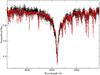 |
Fig. 5 Comparison of a single observed composite spectrum (black circles) to the disentangled spectrum of the primary component (red lines), which illustrates the significant increase in S/N that is obtained. |
For the spectrum analysis of both components of KIC 11285625, we used the GSSP code (Grid Search in Stellar Parameters, Tkachenko et al. 2012) that finds the optimum values of Teff, log g, ξ, [M/H], and vsini from the minimum in χ2 obtained from a comparison of the observed spectrum with the synthetic ones computed from all possible combinations of the above parameters. The errors of measurement (1σ confidence level) are calculated from the χ2 statistics using the projections of the hypersurface of the χ2 from all grid points of all parameters in question. In this way, the estimated error bars include any possible model-inherent correlations between the parameters but do not consider imperfections of the model (such as incorrect atomic data, non-LTE effects, etc.) and/or continuum normalization. A detailed description of the method and its application to the spectra of Kepler β Cep and SPB candidate stars and δ Sct and γ Dor candidate stars are given in Lehmann et al. (2011) and Tkachenko et al. (2012), respectively.
For the calculation of synthetic spectra, we used the LTE-based code SynthV (Tsymbal 1996) which allows the computation of the spectra based on individual elemental abundances. The code uses calculated atmosphere models which have been computed with the most recent, parallelised version of the LLmodels program (Shulyak et al. 2004). Both programs make use of the VALD database (Kupka et al. 2000) for a selection of atomic spectral lines. The main limitation of the LLmodels code is that the models are well suited to early and intermediate spectral type stars but not for very hot and cool stars where non-LTE effects or absorption in molecular bands may become relevant, respectively.
Given that KIC 11285625 is an eclipsing, double-lined (SB2) spectroscopic binary for which unprecedented quality (Kepler) photometry is available, the masses and the radii of both components were determined with very high precision. Having those two parameters, we evaluated surface gravities of the two stars with far better precision than one would expect from the spectroscopic analysis, given that the S/N of our spectra varies between 40 and 70 (this depends on the weather conditions on the night when the observations were taken). Thus, we fixed log g for both components to their photometric values (3.97 and 4.18 for the primary and secondary, respectively) and adjusted the effective temperature Teff, micro-turbulent velocity ξ, projected rotational velocity vsini, and overall metallicity [M/H] for both stars based on their disentangled spectra. Given that the contribution of the primary component to the total light of the system is significantly larger than that of the secondary component (72% compared to 28%) and that its decomposed spectrum is consequently better defined and is of higher quality than that of the secondary component, we were not only able to evaluate individual abundances for this star but also the fundamental atmospheric parameters. Table 2 lists the fundamental parameters of the two stars, whereas Table 3 summarizes the results of chemical composition analysis for the primary component. The overall metallicities of the two stars agree within the quoted errors, but the derived temperature for the secondary component is not reliable, since we find it to be about 200 K hotter than the primary. From the relative eclipse depths, we estimate the temperature of the secondary to be about 6400 K. The cause of this temperature discrepancy is the poor quality of the disentangled spectrum of the secondary component, given its smaller light contribution. Normalization errors in the spectra can easily translate into temperature errors of several hundred Kelvin. Note that the listed uncertainties for the spectroscopic temperatures do not consider normalization errors.
Figure 6 shows the position of the primary component in the log (Teff)-log g diagram with respect to the observational δ Sct (solid lines) and γ Dor (dashed lines) instability strips, as given by Rodríguez & Breger (2001) and Handler & Shobbrook (2002), respectively. The primary falls into the γ Dor instability strip, meaning that pure g-modes are expected to be excited in its interior.
Fundamental parameters of both components of KIC 11285625.
Atmospheric chemical composition of the primary component of KIC 11285625.
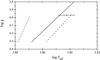 |
Fig. 6 Location of the primary of KIC 11285625 in the log (Teff) – log g diagram. The γ Dor and the red edge of the δ Sct observational instability strips are represented by the dashed and solid lines, correspondingly. According to the photometric Teff and log g, the secondary component would be located in the lower right corner of the diagram, outside both instability strips. |
6. Pulsation spectrum
Figure 7 shows the amplitude spectrum of the Kepler light curve with the binary model removed in the region 0–2 d-1, where most of the dominant pulsation frequencies are found. Clearly visible are the three groups of peaks around 0.557, 1.124 and 1.684 d-1. Some of the frequencies found in the groups around 1.124 and 1.684 d-1 are harmonics of frequencies present in the group around 0.557 d-1. These harmonics are caused by the non-linear nature of the pulsations and have been observed for many pulsators observed by CoRoT and Kepler along almost the entire main-sequence (Degroote et al. 2009; Poretti et al. 2011; Breger et al. 2011; Balona 2012) and have been observed for γ Dor stars in particular (Tkachenko et al. 2013). Closer inspection of the main frequency groups revealed that they consist of several closely spaced peaks, which are almost equally spaced with a frequency of ~0.010 d-1. A likely explanation is amplitude modulation of the pulsation signal on a timescale of ~100 days. Mathematically, the effect of amplitude modulation can be described as follows: Imagine a simplified case where a single periodic non-linear pulsation signal is being modulated with a general periodic function. We can write this signal as a product of two sums of sines, where the number of terms (harmonics) in each sum depends on how non-linear (non-sinusoidal) the signals are: ![\begin{equation} \sum_{i=1}^{N_\mathrm{mod}} a_\mathrm{i} \sin{\left[2\pi f_\mathrm{mod} i t + \phi^\mathrm{mod}_\mathrm{i}\right]} \sum_{j=1}^{N_\mathrm{puls}} b_\mathrm{j} \sin{\left[2\pi f_\mathrm{puls} j t + \phi^\mathrm{puls}_\mathrm{j}\right]} , \end{equation}](/articles/aa/full_html/2013/08/aa21702-13/aa21702-13-eq55.png) (1)where fmod is the modulation frequency and fpuls the pulsation frequency. This product can be rewritten as a sum using Simpsons rule:
(1)where fmod is the modulation frequency and fpuls the pulsation frequency. This product can be rewritten as a sum using Simpsons rule: ![\begin{eqnarray} \sum_{i=1}^{N_\mathrm{mod}} \sum_{j=1}^{N_\mathrm{puls}} \frac{a_\mathrm{i} b_\mathrm{j}}{2}\left(\cos{\left[2\pi \left(f_\mathrm{puls} j-f_\mathrm{mod} i\right)t+\phi^\mathrm{puls}_\mathrm{j}-\phi^\mathrm{mod}_\mathrm{i}\right]}\right.\\\left. -\cos{\left[2\pi \left(f_\mathrm{puls} j+f_\mathrm{mod} i\right)t+\phi^\mathrm{puls}_\mathrm{j}+\phi^\mathrm{mod}_\mathrm{i}\right]}\right). \nonumber \end{eqnarray}](/articles/aa/full_html/2013/08/aa21702-13/aa21702-13-eq58.png) (2)In the Fourier transform of this signal, we will thus see peaks at frequencies which are linear combinations of the pulsation frequency and the modulation frequency, where the number of combinations depends on how non-linear both signals are. Most of the observed substructure in the amplitude spectrum can be explained by amplitude modulation of a pulsation signal with fmod ~ 0.010 d-1. A more detailed description of amplitude and frequency modulation in light curves can be found in Benkó et al. (2011). Since the period of the amplitude modulation is close to the length of a Kepler observing quarter, we checked for a possible instrumental origin. A very strong argument against this is that the modulation is not present in the eclipse signal of the light curve but is only affecting the pulsation peaks.
(2)In the Fourier transform of this signal, we will thus see peaks at frequencies which are linear combinations of the pulsation frequency and the modulation frequency, where the number of combinations depends on how non-linear both signals are. Most of the observed substructure in the amplitude spectrum can be explained by amplitude modulation of a pulsation signal with fmod ~ 0.010 d-1. A more detailed description of amplitude and frequency modulation in light curves can be found in Benkó et al. (2011). Since the period of the amplitude modulation is close to the length of a Kepler observing quarter, we checked for a possible instrumental origin. A very strong argument against this is that the modulation is not present in the eclipse signal of the light curve but is only affecting the pulsation peaks.
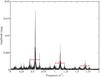 |
Fig. 7 Part of the amplitude spectrum (below 2 d-1) of the Kepler light curve with the binary model removed. The red arrows indicate the splitting of groups of peaks caused by rotation with a splitting value around 0.1 d-1. |
Dominant fifty frequencies with their amplitude and S/N as detected in the Kepler light curve with the binary model removed, using the prewhitening technique as explained in the text.
To study the pulsation signal in detail, we performed a complete frequency analysis using an iterative prewhitening procedure. The Lomb-Scargle periodogram was used in combination with false-alarm probabilities to detect the significant frequencies present in the light curve. Prewhitening of the frequencies was performed using linear least-squares fitting with non-linear refinement. In total, hundreds of formally significant frequencies were detected. We stress here that formal significance does not imply that a frequency has a physical interpretation, e.g. in the sense of all being independent pulsation modes. Most of them are not independent at all; many combination frequencies and harmonics are present and many peaks arise because we perform Fourier analysis on a signal that is not strictly periodic. Table 4 lists the 50 most significant frequencies with their amplitude and estimated S/N. The noise level used to calculate the S/N was estimated from the average amplitude in the frequency range between 20 and 24 d-1. The last column indicates possible combination frequencies and harmonics. The lowest order combination is always listed. However, some frequencies can be written equivalently as a different higher order combination of more dominant frequencies (they are listed in brackets). A complete list of frequencies is available online in electronic format at the CDS3. Clearly, many frequencies can be explained by low-order linear combinations of the three most dominant frequencies. However, these dominant frequencies are likely not independent (corresponding to different pulsation modes) given the amplitude modulation. Instead, they are probably combination frequencies of the real pulsation frequency and (harmonics of) the modulation frequency fmod ~ 0.010 d-1. Looking back at the RV data for the pulsating component, we expect the larger scatter in comparison to the secondary component to be caused by the pulsations. After subtraction of the Keplerian orbit fit, we analysed the frequencies in the residuals and found two significant peaks corresponding to frequencies detected in the Kepler data (f1 and f7 in Table 4). The amplitude spectra of the RV residuals for both components are shown in Fig. 9.
Frequency differences and corresponding periods (in order of decreasing occurrence) as detected in the list of the first 400 frequencies obtained using iterative prewhitening.
From spectroscopy, we found vsini = 14.2 ± 1.5 km s-1 for the pulsating primary component and vsini = 8.4 ± 1.5 km s-1 for the secondary component. Assuming that the rotation axes are perpendicular to the orbital plane and using the orbital and stellar parameters listed in Table 1, this corresponds to a rotation period of about 7.5 ± 1.3 d for the primary and 8.8 ± 1.9 d for the secondary component. These values suggest super-synchronous rotation, but do not provide sufficient evidence on their own, given the uncertainties (1σ), especially not for the secondary component.
We analysed the pulsation signal to detect signs of rotational splitting of the pulsation frequencies in two different ways: by computing the autocorrelation function of the amplitude spectrum and by using the list of detected significant frequencies. The autocorrelation function between 0 and 0.7 d-1 is shown in Fig. 8. Clearly, the amplitude spectrum is self-similar for many different frequency shifts, as is shown by the complex structure of the autocorrelation function. Although the autocorrelation function is dominated by the highest peaks in the amplitude spectrum and their higher harmonics, we can relate some smaller peaks to the properties of the system. For example, the peaks indicated with the red arrows correspond to the orbital frequency and the rotational frequency of the primary as derived from spectroscopy (at 0.0926 and 0.1333 d-1 respectively).
Next, we searched the list of significant frequencies for any possible frequency differences that occur several times (given the frequency resolution). In this way, splittings of lower amplitude peaks can be detected more easily, which is not the case when using the autocorrelation function. Since the number of significant frequencies is so large, several frequency differences occur multiple times purely by chance (this was checked by using a list of randomly generated frequencies), so one must be careful when interpreting the results (see e.g. Pápics 2012). In our search for splittings, we used frequency lists of different lengths, ranging from the first 50 to a maximum of several hundred significant frequencies (down to a S/N of 10). We used a rather strict cutoff value of 0.0001 d-1 to accept frequency differences as being equal (0.1/T, with T the total time span of the light curve). Next, we ordered all possible frequency differences in increasing order of occurrence. This always resulted in the same differences showing up in the top of the lists. Table 5 shows the most abundant differences detected in a conservative list of only 400 frequencies (down to a S/N of about 50). Clearly, many of these differences are related to the amplitude modulation in the light curve (as discussed above), with values around 0.010 d-1 (suspected modulation frequency) and 0.020 d-1 (twice the modulation frequency) occurring often. Values around 0.567 d-1 are related to the presence of higher harmonics of the pulsation frequencies. In the autocorrelation function, clear peaks are present around the orbital frequency, while the orbital frequency itself only shows up in the list of frequency differences when going down to S/N values around 10. Most likely, this is caused by small residuals of the binary signal (eclipses) in the light curve. We also find values very close to the rotation frequency from spectroscopy and values in between the rotation frequency and the orbital frequency. They are also visible as the group of peaks in the autocorrelation function around 0.1 d-1. We interpret these as the result of rotational splitting. The values are compatible with the spectroscopic results obtained for the primary, and hence provide stronger evidence of super-synchronous rotation. We cannot unambiguously identify one unique rotational splitting but rather a range of possible values. The difference in measured splitting values across the spectrum suggests non-rigid rotation in the interior of the primary (see e. g. Aerts et al. 2003, 2010; Dziembowski & Pamyatnykh 2008).
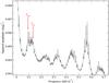 |
Fig. 8 Autocorrelation of the amplitude spectrum after removal of the binary model. |
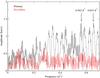 |
Fig. 9 Amplitude spectrum of the RV residuals for both components after subtraction of the best Keplerian orbit fit. The two highest peaks for the primary (indicated) correspond to frequencies detected in the Kepler light curve. |
In Fig. 7, the structures in the amplitude spectrum caused by rotational splitting are indicated by means of red arrows. Clearly, the pattern is repeated for the higher harmonics of the pulsation frequencies.
Finally, the second-most dominant peak in the amplitude spectrum almost coincides with the sixth harmonic of the orbital frequency. This suggests tidally affected pulsation, although this is not expected for non-eccentric systems. Moreover, the frequencies do not match perfectly, and the second-most dominant peak is likely not an independent pulsation mode, but caused by the amplitude modulation of the main oscillation frequency.
7. Conclusions
We have obtained accurate system parameters and astrophysical properties for KIC 11285625, a double-lined eclipsing binary system with a γ Dor pulsator discovered by the Kepler space mission. The excellent Kepler data with a total time span of almost 1000 days have been analysed in combination with high resolution HERMES spectra. The individual composite spectra could not be used to derive fundamental parameters, such as Teff and log g, given their insufficient S/N. This was achieved after using the spectral disentangling technique for both components.
An iterative automated method was developed to separate the orbital variability in the Kepler light curve from the variability due to the pulsations of the primary. Because the orbital frequency and its overtones are located in the same frequency range as the pulsation frequencies, a simple separation technique (such as a filter in the frequency domain) was insufficient. We plan to develop this technique further and apply it to other binary systems in the Kepler database.
After removal of the best binary model, we studied the residual pulsation signal in detail and found indications for rotational splitting of the pulsation frequencies, which are compatible with super-synchronous and non-rigid internal rotation. A detailed asteroseismic analysis of the γ Dor pulsator and comparison with theoretical models can now be attempted on the basis of this observational work, which constitutes an excellent starting point for stellar modelling of a γ Dor star. A concrete interpretation of the detected amplitude modulation must await a much longerKepler light curve, given the relatively long modulation period.
Centre de Données astronomiques de Strasbourg, http://cdsweb.u-strasbg.fr/
Acknowledgments
The research leading to these results has received funding from the European Research Council under the European Community’s Seventh Framework Programme (FP7/2007–2013)/ERC grant agreement No. 227224 (PROSPERITY), from the Research Council of K.U. Leuven (GOA/2008/04), and from the Belgian federal science policy office (C90309: CoRoT Data Exploitation); A. Tkachenko and P. Degroote are postdoctoral fellows of the Fund for Scientific Research (FWO), Flanders, Belgium. Funding for the Kepler Discovery mission is provided by NASA’s Science Mission Directorate. Some of the data presented in this paper were obtained from the Multimission Archive at the Space Telescope Science Institute (MAST). STScI is operated by the Association of Universities for Research in Astronomy, Inc., under NASA contract NAS5-26555. Support for MAST for non-HST data is provided by the NASA Office of Space Science via grant NNX09AF08G and by other grants and contracts. This research has made use of the SIMBAD database, operated at CDS, Strasbourg, France. We would like to express our special thanks to the numerous people who helped make the Kepler mission possible.
References
- Aerts, C., Thoul, A., Daszyńska, J., et al. 2003, Science, 300, 1926 [NASA ADS] [CrossRef] [PubMed] [Google Scholar]
- Aerts, C., Christensen-Dalsgaard, J., & Kurtz, D. W. 2010, Asteroseismology (Springer) [Google Scholar]
- Balona, L. A. 2012, MNRAS, 422, 1092 [NASA ADS] [CrossRef] [Google Scholar]
- Benkó, J. M., Szabó, R., & Paparó, M. 2011, MNRAS, 417, 974 [NASA ADS] [CrossRef] [Google Scholar]
- Borucki, W. J., Koch, D., Basri, G., et al. 2010, Science, 327, 977 [NASA ADS] [CrossRef] [PubMed] [Google Scholar]
- Breger, M., Balona, L., Lenz, P., et al. 2011, MNRAS, 414, 1721 [NASA ADS] [CrossRef] [Google Scholar]
- Debosscher, J., Blomme, J., Aerts, C., & De Ridder, J. 2011, A&A, 529, A89 [NASA ADS] [CrossRef] [EDP Sciences] [Google Scholar]
- Degroote, P., Briquet, M., Catala, C., et al. 2009, A&A, 506, 111 [NASA ADS] [CrossRef] [EDP Sciences] [Google Scholar]
- Dziembowski, W. A., & Pamyatnykh, A. A. 2008, MNRAS, 385, 2061 [NASA ADS] [CrossRef] [Google Scholar]
- Etzel, P. B. 1981, in Photometric and Spectroscopic Binary Systems, eds. E. B. Carling, & Z. Kopal, 111 [Google Scholar]
- Grevesse, N., Asplund, M., & Sauval, A. J. 2007, Space Sci. Rev., 130, 105 [Google Scholar]
- Hadrava, P. 1995, A&AS, 114, 393 [NASA ADS] [Google Scholar]
- Handler, G., & Shobbrook, R. R. 2002, MNRAS, 333, 251 [NASA ADS] [CrossRef] [Google Scholar]
- Hensberge, H., Pavlovski, K., & Verschueren, W. 2000, A&A, 358, 553 [NASA ADS] [Google Scholar]
- Ilijic, S., Hensberge, H., Pavlovski, K., & Freyhammer, L. M. 2004, in Spectroscopically and Spatially Resolving the Components of the Close Binary Stars, eds. R. W. Hilditch, H. Hensberge, & K. Pavlovski, ASP Conf. Ser., 318, 111 [Google Scholar]
- Kupka, F. G., Ryabchikova, T. A., Piskunov, N. E., Stempels, H. C., & Weiss, W. W. 2000, Baltic Astron., 9, 590 [Google Scholar]
- Lehmann, H., Tkachenko, A., Semaan, T., et al. 2011, A&A, 526, A124 [NASA ADS] [CrossRef] [EDP Sciences] [Google Scholar]
- Maceroni, C., Montalbán, J., Michel, E., et al. 2009, A&A, 508, 1375 [NASA ADS] [CrossRef] [EDP Sciences] [Google Scholar]
- Maceroni, C., Montalbán, J., Gandolfi, D., Pavlovski, K., & Rainer, M. 2013, A&A, 552, A60 [NASA ADS] [CrossRef] [EDP Sciences] [Google Scholar]
- Pápics, P. I. 2012, Astron. Nachr., 333, 1053 [NASA ADS] [CrossRef] [Google Scholar]
- Pavlovski, K., & Hensberge, H. 2005, A&A, 439, 309 [NASA ADS] [CrossRef] [EDP Sciences] [Google Scholar]
- Popper, D. M., & Etzel, P. B. 1981, AJ, 86, 102 [NASA ADS] [CrossRef] [Google Scholar]
- Poretti, E., Rainer, M., Weiss, W. W., et al. 2011, A&A, 528, A147 [NASA ADS] [CrossRef] [EDP Sciences] [Google Scholar]
- Prša, A., Batalha, N., Slawson, R. W., et al. 2011, AJ, 141, 83 [NASA ADS] [CrossRef] [Google Scholar]
- Raskin, G., van Winckel, H., Hensberge, H., et al. 2011, A&A, 526, A69 [NASA ADS] [CrossRef] [EDP Sciences] [Google Scholar]
- Rodríguez, E., & Breger, M. 2001, A&A, 366, 178 [NASA ADS] [CrossRef] [EDP Sciences] [Google Scholar]
- Shulyak, D., Tsymbal, V., Ryabchikova, T., Stütz, C., & Weiss, W. W. 2004, A&A, 428, 993 [NASA ADS] [CrossRef] [EDP Sciences] [Google Scholar]
- Simon, K. P., & Sturm, E. 1994, A&A, 281, 286 [NASA ADS] [Google Scholar]
- Southworth, J., Maxted, P. F. L., & Smalley, B. 2004a, MNRAS, 351, 1277 [NASA ADS] [CrossRef] [Google Scholar]
- Southworth, J., Zucker, S., Maxted, P. F. L., & Smalley, B. 2004b, MNRAS, 355, 986 [NASA ADS] [CrossRef] [Google Scholar]
- Tkachenko, A., Lehmann, H., Smalley, B., Debosscher, J., & Aerts, C. 2012, MNRAS, 422, 2960 [NASA ADS] [CrossRef] [Google Scholar]
- Tkachenko, A., Aerts, C., Yakushechkin, A., et al. 2013, A&A, 556, A52 [NASA ADS] [CrossRef] [EDP Sciences] [Google Scholar]
- Tsymbal, V. 1996, in M.A.S.S., Model Atmospheres and Spectrum Synthesis, eds. S. J. Adelman, F. Kupka, & W. W. Weiss, ASP Conf. Ser., 108, 198 [Google Scholar]
- Welsh, W. F., Orosz, J. A., Aerts, C., et al. 2011, ApJS, 197, 4 [NASA ADS] [CrossRef] [Google Scholar]
All Tables
Orbital and physical parameters for both components of KIC 11285625 obtained from the combined spectroscopic and photometric analysis.
Dominant fifty frequencies with their amplitude and S/N as detected in the Kepler light curve with the binary model removed, using the prewhitening technique as explained in the text.
Frequency differences and corresponding periods (in order of decreasing occurrence) as detected in the list of the first 400 frequencies obtained using iterative prewhitening.
All Figures
|
Fig. 1 Combination of observing quarters Q1-Q10 for KIC 11285625. The top panel shows the raw SAP (simple aperture photometry) fluxes, as they were delivered, while the lower panel shows the resulting combined dataset after optimal mask selection and detrending. |
| In the text | |
|
Fig. 2 Kepler aperture (left) and a single target pixel image (right) for KIC 11285625 at quarter Q3. Red colours in the pixel image indicate the lowest flux levels, white colours indicate the highest flux levels. |
| In the text | |
|
Fig. 3 Upper panel: phased HERMES RV data (open circles) and Keplerian model fits (lines) for both components (black: primary, red: secondary). Middle panel: phased Kepler data (pulsations removed) with the binary model overplotted in red. Lower panel: phased residuals of the Kepler data after removal of both the pulsations and the binary model. |
| In the text | |
|
Fig. 4 Upper panel: resulting light curve after iterative removal of the orbital variability (in red) with the original light curve shown for comparison (in black). Lower panel: amplitude spectrum of the original Kepler light curve (in black) and the amplitude spectrum of the pulsation “residuals” (in red) after iterative removal of the orbital variability. |
| In the text | |
|
Fig. 5 Comparison of a single observed composite spectrum (black circles) to the disentangled spectrum of the primary component (red lines), which illustrates the significant increase in S/N that is obtained. |
| In the text | |
|
Fig. 6 Location of the primary of KIC 11285625 in the log (Teff) – log g diagram. The γ Dor and the red edge of the δ Sct observational instability strips are represented by the dashed and solid lines, correspondingly. According to the photometric Teff and log g, the secondary component would be located in the lower right corner of the diagram, outside both instability strips. |
| In the text | |
|
Fig. 7 Part of the amplitude spectrum (below 2 d-1) of the Kepler light curve with the binary model removed. The red arrows indicate the splitting of groups of peaks caused by rotation with a splitting value around 0.1 d-1. |
| In the text | |
|
Fig. 8 Autocorrelation of the amplitude spectrum after removal of the binary model. |
| In the text | |
|
Fig. 9 Amplitude spectrum of the RV residuals for both components after subtraction of the best Keplerian orbit fit. The two highest peaks for the primary (indicated) correspond to frequencies detected in the Kepler light curve. |
| In the text | |
Current usage metrics show cumulative count of Article Views (full-text article views including HTML views, PDF and ePub downloads, according to the available data) and Abstracts Views on Vision4Press platform.
Data correspond to usage on the plateform after 2015. The current usage metrics is available 48-96 hours after online publication and is updated daily on week days.
Initial download of the metrics may take a while.