| Issue |
A&A
Volume 556, August 2013
|
|
|---|---|---|
| Article Number | A40 | |
| Number of page(s) | 6 | |
| Section | Numerical methods and codes | |
| DOI | https://doi.org/10.1051/0004-6361/201220458 | |
| Published online | 23 July 2013 | |
Non-symmetric magnetohydrostatic equilibria: a multigrid approach
1
School of Engineering, Computing and Applied Mathematics, University of
Abertay Dundee,
Kydd Building,
Dundee,
DD1 1HG
UK
e-mail:
This email address is being protected from spambots. You need JavaScript enabled to view it.
2
Department of Mathematics and Information Sciences, Northumbria
University, Newcastle Upon
Tyne, NE1 8ST,
UK
3
School of Mathematics and Statistics, University of Glasgow,
Glasgow,
G12 8QW,
UK
Received:
6
May
2013
Accepted:
23
June
2013
Abstract
Aims. Linear magnetohydrostatic (MHS) models of solar magnetic fields balance plasma pressure gradients, gravity and Lorentz forces where the current density is composed of a linear force-free component and a cross-field component that depends on gravitational stratification. In this paper, we investigate an efficient numerical procedure for calculating such equilibria.
Methods. The MHS equations are reduced to two scalar elliptic equations – one on the lower boundary and the other within the interior of the computational domain. The normal component of the magnetic field is prescribed on the lower boundary and a multigrid method is applied on both this boundary and within the domain to find the poloidal scalar potential. Once solved to a desired accuracy, the magnetic field, plasma pressure and density are found using a finite difference method.
Results. We investigate the effects of the cross-field currents on the linear MHS equilibria. Force-free and non-force-free examples are given to demonstrate the numerical scheme and an analysis of speed-up due to parallelization on a graphics processing unit (GPU) is presented. It is shown that speed-ups of ×30 are readily achievable.
Key words: magnetic fields / magnetohydrodynamics (MHD) / methods: numerical
© ESO, 2013
1. Introduction
The calculation of three-dimensional non-linear magnetohydrostatic (MHS) equilibria is a non-trivial subject. In the solar physics context, progress has been made by considering linear subclasses of MHS equilibria. One such class, known as laminated equilibria, makes use of an Euler potential representation of the magnetic field (e.g. Low 1982). On each lamina, a 2D magnetic field is calculated and the 3D field comprises of the union of these laminas.
Another approach is to model the current density as a linear combination of field-aligned and cross-field currents (Low 1991, 1992). Here, the field-aligned current is that of a linear force-free field and the cross-field current depends on the variation of the magnetic field with height. Details of this will be presented in the next section. Neukirch & Rastätter (1999; NR99 hereafter) present a new formulation of Low’s model by writing the magnetic field in terms of poloidal and toroidal components. This has the advantage that the calculation of the magnetic field only involves one scalar function whereas, previously, one was forced to operate with all three components of the magnetic field independently. Petrie & Neukirch (2000) use the representation of NR99 and find closed-form solutions for MHS equilibria via Green’s functions. The price paid for finding closed-form solutions, however, is that they are forced to choose a simple term for the cross-field current. To date, the authors are unaware of any closed-form solutions using Green’s functions, other than those presented in Petrie & Neukirch (2000).
Although more detailed analytical solutions may prove difficult with the representation of NR99, it is, however, set up perfectly for an efficient numerical treatment. In this paper, we outline a simple and fast numerical procedure for calculating MHS equilibria based on the NR99 representation. The details of this are given in the next section. This is followed by some examples of force-free and linear MHS equilibria. For the linear MHS case, we investigate the effects of the cross-field currents on the equilibria. We then highlight how the scheme can be parallelized simply and effectively on a graphics processing unit (GPU). The paper concludes with a summary.
2. Model equations and solution method
Firstly, we shall outline where the equations to be solved come from. Fuller details can be found in NR99. This will be followed by an algorithm for the numerical solution.
2.1. The model equations
The MHS equations that we shall solve are
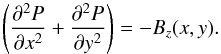
![Mathematical equation: \begin{eqnarray} \label{mhs1} &&\mu_0^{-1}(\nabla\times\vec{B})\times\vec{B} -\nabla p - \rho g\hat{\vec{e}}_z = \vec{0}, \\[3mm] \label{mhs2} &&\nabla\times\vec{B} = \mu_0\vec{j}, \\[3mm] \label{mhs3} &&\nabla\cdot\vec{B} = 0, \end{eqnarray}](/articles/aa/full_html/2013/08/aa20458-12/aa20458-12-eq2.png)
where B is the magnetic induction (commonly referred to as the magnetic
field), j is the current density, p is the plasma presure,
ρ is the density, g is the (constant) gravitational
acceleration and μ0 is the permeability of free space. To
complete the problem, boundary conditions must be specified. This choice is
problem-dependent but will, at least, require B to be specified on the
boundaries of the domain through Dirichlet or von Neuman conditions. In this paper we will
consider a Cartesian domain. Following Low (1992),
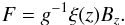
we assume the current density takes the following form 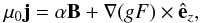 (4)where
α is a constant and F is an arbitrary function. The
first term on the right-hand-side is the aligned current associated with a linear
force-free field. The second term is the non-force-free cross current due to the
gravitational stratification. The magnetic induction can be written as
(4)where
α is a constant and F is an arbitrary function. The
first term on the right-hand-side is the aligned current associated with a linear
force-free field. The second term is the non-force-free cross current due to the
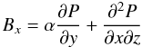
gravitational stratification. The magnetic induction can be written as ![Mathematical equation: \begin{equation} \label{b_iden} \vec{B} = \nabla\times[\nabla\times(P\hat{\vec{e}}_z) + T\hat{\vec{e}}_z], \end{equation}](/articles/aa/full_html/2013/08/aa20458-12/aa20458-12-eq12.png) (5)where
P and T are scalar functions corresponding to the
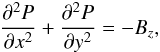
poloidal and toroidal components respectively. This form satisfies Eq. (3). Using this in Eq. (2) with Eq. (4) gives
(5)where
P and T are scalar functions corresponding to the
poloidal and toroidal components respectively. This form satisfies Eq. (3). Using this in Eq. (2) with Eq. (4) gives
![Mathematical equation: \begin{eqnarray} \label{t} &&T = \alpha P, \\[2mm] \label{helm} &&\nabla^2P + \alpha^2 P + gF = 0. \end{eqnarray}](/articles/aa/full_html/2013/08/aa20458-12/aa20458-12-eq15.png)
Following NR99 and Low (1992), we set
 With this identity,
Eq. (7) becomes
With this identity,
Eq. (7) becomes ![Mathematical equation: \begin{equation} \label{scalar_pot} [1-\xi(z)]\left(\frac{\partial^2P}{\partial x^2} +\frac{\partial^2P}{\partial y^2}\right) + \frac{\partial^2P}{\partial z^2} + \alpha^2 P = 0. \end{equation}](/articles/aa/full_html/2013/08/aa20458-12/aa20458-12-eq17.png) (8)For
ξ(z) < 1, Eq. (8) is elliptic. Now the magnetic field can be
found by solving this for the poloidal scalar potential P and then using
Eqs. (5) and (6).
(8)For
ξ(z) < 1, Eq. (8) is elliptic. Now the magnetic field can be
found by solving this for the poloidal scalar potential P and then using
Eqs. (5) and (6).
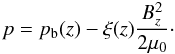
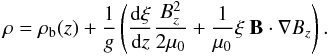
Once the magnetic field is found, the plasma pressure and density are given by
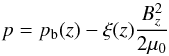 (9)and
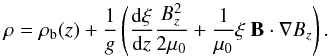 (10)pb
and ρb are the background equilibrium plasma pressure and
density respectively. A derivation of these formulae is given in NR99.
(10)pb
and ρb are the background equilibrium plasma pressure and
density respectively. A derivation of these formulae is given in NR99.
2.2. The numerical procedure
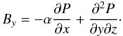
An efficient numerical solution of this class of the MHS equations rests on reducing the equations to a set of linear, scalar elliptic problems. I.e. those of the form
 with u
defined on
with u
defined on  .
Here the Laplacian operator can be two-dimensional (for boundaries) or three-dimensional
(for the interior) and a, b and c are
known scalar functions.
.
Here the Laplacian operator can be two-dimensional (for boundaries) or three-dimensional
(for the interior) and a, b and c are
known scalar functions.
There exists a wide variety of techniques to solve such problems efficiently, from Krylov subspace methods to multigrid methods. Although solution methods are problem-dependent, the multigrid method is often an optimal solver for discrete Poisson problems (Elman et al. 2005), i.e. its convergence rate is independent of the problem mesh size. It can also be parallelized efficiently, and for these reasons we adopt it in this work. The multigrid method, in a different representation to the one of this paper, was used successfully for MHS models of flux tubes bounded by current sheets (Henning & Cally 2001).
As mentioned above, the MHS equations are reduced to a set of linear elliptic problems
defined on the boundaries and in the interior. Equation (8) is the three-dimensional elliptic problem for the poloidal scalar
potential P defined in the interior of the domain. The other elliptic
equations required to be solved depend on the boundary conditions. On the lower boundary,
the vertical component of the magnetic field,
Bz, is prescribed. From Eq. (5), it is clear that, on the lower boundary,
 (11)In principle other
elliptic equtions can be defined on the other boundaries of the Cartesian domain. For
simplicity, however, we shall assume the B = 0 on these
boundaries. For the scalar elliptic problem, this translates to P = 0 on
top and side boundaries. This boundary condition also applies to the sides of the 2D
domain (the lower boundary) where Eq. (11)
is solved. In short, the numerical procedure to determine the poloidal scalar potential
P involves:
(11)In principle other
elliptic equtions can be defined on the other boundaries of the Cartesian domain. For
simplicity, however, we shall assume the B = 0 on these
boundaries. For the scalar elliptic problem, this translates to P = 0 on
top and side boundaries. This boundary condition also applies to the sides of the 2D
domain (the lower boundary) where Eq. (11)
is solved. In short, the numerical procedure to determine the poloidal scalar potential
P involves:
-
1.
Set P = 0 everywhere, initially, on the grid.
-
2.
Use the multigrid method to solve Eq. (11) on the lower boundary with P = 0 on the sides.
-
3.
Use the multigrid method to solve Eq. (8) within the domain, using P = 0 on the top and side boundaries and the distribution of P on the lower boundary determined from the previous step.
After these steps are completed, the magnetic field B can be calculated. From Eq. (5), the other components of the magnetic field are given by
 and
and
 These, together
with Eq. (11), can be approximated using
finite differences, giving Bx,
By and
Bz on the grid to a required accuracy. In
this paper, we use second-order accurate central finite differences.
These, together
with Eq. (11), can be approximated using
finite differences, giving Bx,
By and
Bz on the grid to a required accuracy. In
this paper, we use second-order accurate central finite differences.
All that remains now is the calculation of the pressure p and the density ρ. Once Bz is determined on the grid, it is clear from Eq. (9) that p can be evaluated directly. In Eq. (10) the derivatives must be dealt with using finite differences. After this, ρ is determined on the grid.
3. Examples
Here we present examples of equilibria to demonstrate the effectiveness of our numerical scheme. Details of computational aspects and parallelization are discussed in Sect. 4.
For the cases under consideration we non-dimensionalize Eqs. (1) to (3) with respect to photospheric values. The variables are plasma pressure, p0 = 1.4 × 10⁴ Pa; density, ρ0 = 3 × 10⁻⁴ kg/m3; scale height H0 = 340 km; magnetic induction B0 = (2μ0p0)1/2 = 1.3 × 10³ G and temperature, T0 = p0/(Rρ0) = 5.6 × 10³ K. Here, R is the gas constant.
We assume a background temperature profile of the form
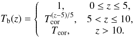 Tcor = 150
is the non-dimensional coronal temperature. The model photosphere/chromosphere ranges from
0 ≤ z ≤ 5, the transition region ranges from
5 < z ≤ 10 and the corona is in
z > 10. With an ideal gas equation
Tcor = 150
is the non-dimensional coronal temperature. The model photosphere/chromosphere ranges from
0 ≤ z ≤ 5, the transition region ranges from
5 < z ≤ 10 and the corona is in
z > 10. With an ideal gas equation
 hydrostatic pressure
balance can be written as
hydrostatic pressure
balance can be written as
 The equation is
solved for pb and then ρb follows
from the ideal gas law. The non-dimensionalization and atmospheric model presented here are
similar to those in flux emergence studies (e.g. MacTaggart
2011; Hood et al. 2012; McLaughlin et al. 2012). For the following cases, we set
B = 0 on the side and top boundaries. The size of the domain is
[−5.5,5.5] 2 × [0,12] and we use a
resolution of 1283.
The equation is
solved for pb and then ρb follows
from the ideal gas law. The non-dimensionalization and atmospheric model presented here are
similar to those in flux emergence studies (e.g. MacTaggart
2011; Hood et al. 2012; McLaughlin et al. 2012). For the following cases, we set
B = 0 on the side and top boundaries. The size of the domain is
[−5.5,5.5] 2 × [0,12] and we use a
resolution of 1283.
3.1. Force-free case
For a force-free field, ξ = 0. This, of course, means that p = pb and ρ = ρb. In this example we take α = 0.4. We model a magnetic configuration with three sources, similar to that in Régnier et al. (2005). For each source, we define a Gaussian profile for Bz, on the lower boundary, of the form
 B0
is the field strength at the centre of the source, l is source width and
r2 = (x − x0)2 + (y − y0)2
with source centre
(x0,y0). Here
we take l = 0.3 for all the sources. There is one positive source with
Bz = 1 and two negative sources with
Bz = −0.5. The position of the positive
source is (1.5, 1.5). The two negative sources have positions (−1.5, −1.5) and (1.5,
−1.5). Figure 1 shows some field lines of the
calculated region, with a magnetogram of Bz
displayed at the base.
B0
is the field strength at the centre of the source, l is source width and
r2 = (x − x0)2 + (y − y0)2
with source centre
(x0,y0). Here
we take l = 0.3 for all the sources. There is one positive source with
Bz = 1 and two negative sources with
Bz = −0.5. The position of the positive
source is (1.5, 1.5). The two negative sources have positions (−1.5, −1.5) and (1.5,
−1.5). Figure 1 shows some field lines of the
calculated region, with a magnetogram of Bz
displayed at the base.
 |
Fig. 1 Magnetic field lines of the linear force-free region are displayed in orange. A magnetogram of Bz is given at the base to indicate the positions of the sources. |
Between the two negative polarities, there is a rapid divergence in the field lines as they connect down to the positive polarity. This indicates the presence of a null point at the base of the domain. Further evidence for this can found by looking at the distribution of | B | near the base of the domain. Figure 2 displays this at z = 0.1.
 |
Fig. 2 A map of | B |, within the range given on the scale, at z = 0.1. The null point is clearly highlighted between the two negative polarities. |
3.2. Non-force-free case
Having demonstrated that our multigrid scheme can successfully compute linear force-free
equilibria with rapidly changing field lines and null points, we now turn our attention to
the linear MHS case. For this we examine two profiles for ξ:
![Mathematical equation: \begin{eqnarray} \xi_1(z) &=& 0.7\exp(-0.2z), \\[2mm] \xi_2(z) &=& [0.7+0.3\sin(\pi z)]\exp(-0.1z). \end{eqnarray}](/articles/aa/full_html/2013/08/aa20458-12/aa20458-12-eq69.png) These
profiles are displayed in Fig. 3.
ξ1(z) is a simple exponential decay which
models the fact the magnetic field becomes more force-free as one moves from the
photosphere to the corona. ξ2(z) is also
exponentially decaying but has the additional complexity of a sine wave superimposed on
it. Note that both of these profiles satisfy the condition
ξ(z) < 1 to ensure that Eq.
(8) is elliptic.
These
profiles are displayed in Fig. 3.
ξ1(z) is a simple exponential decay which
models the fact the magnetic field becomes more force-free as one moves from the
photosphere to the corona. ξ2(z) is also
exponentially decaying but has the additional complexity of a sine wave superimposed on
it. Note that both of these profiles satisfy the condition
ξ(z) < 1 to ensure that Eq.
(8) is elliptic.
 |
Fig. 3 The profiles of ξ(z) from the cross-field current. |
3.2.1. Magnetic field and current
The sigmoidal magnetic field for profile ξ1 is displayed in Fig. 4. That for ξ2 is in Fig. 5. In both figures, a magnetogram of Bz is placed at z = 0 and the field lines are shaded with | ∇ × B |.
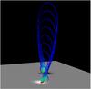 |
Fig. 4 Magnetic field lines for the MHS case with ξ1. The field lines are coloured with | ∇ × B |. |
 |
Fig. 5 Magnetic field lines for the MHS case with ξ2. The field lines are coloured with | ∇ × B |. |
The magnetic field of ξ2 is the more twisted of the two. The current is stronger at the footpoints and this is due to the initial increase in the ξ2 profile. Although the magnetic fields for both profiles look similar, superficially at least, the structure of the current density is different. Figure 6 displays an isosurface of | j | for the ξ1 profile field. Here, the current density is concentrated at the footpoints. Figure 7 displays the corresponding isosurface for the ξ2-profile field. The oscillating ξ2-profile allows for additional structure within the current density, as evidenced by an additional bridging arch in Fig. 7. As one moves higher into the corona, the current density becomes weaker and the magnetic field becomes close to potential.
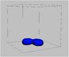 |
Fig. 6 An isosurface of | j| = 0.03 for the MHS solution with ξ1. |
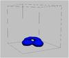 |
Fig. 7 An isosurface of | j| = 0.03 for the MHS solution with ξ2. |
3.2.2. Pressure and density
As is evident from Eqs. (9) and (10), the plasma pressure and density are highly dependent on the magnetic field and the ξ-profile. Although the ξ-profiles are decreasing with height (on average for ξ2), they are always positive. From Eq. (9) it is clear that the effect of a positive ξ-profile is to introduce a pressure deficit where there is strong vertical magnetic field. Since the temperature is constant in the region near the photosphere, the geometrical depression, as measured from the pressure p, corresponds approximately to the Wilson depression (Spruit 1976). For the linear MHS equilibria of this paper, a source of size ≈300 km produces a Wilson depression of ≈100 km. These values lie within the same order of magnitude as those given in Spruit (1976).
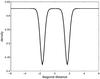 |
Fig. 8 The non-dimensional density along a diagonal cut through the domain at z = 0.46875. The two troughs correspond to the locations of the magnetic footpoints. This profile is for the linear MHS equilibrium with ξ2. |
Equation (10) demonstrates that the
density enhancement or depletion is due to the competition of a magnetic pressure term
combined with ξ′(z) and a magnetic tension
term. Considering the ξ1-profile first,
 for all z.
Hence, the “pressure” term is negative. The “tension” term is also negative due to the
fast drop in field strength of Bz with
height. For the ξ2-profile the situation is slightly more
complex as
for all z.
Hence, the “pressure” term is negative. The “tension” term is also negative due to the
fast drop in field strength of Bz with
height. For the ξ2-profile the situation is slightly more
complex as  is zero, positive and
negative at different heights. This means that the “pressure” term changes sign with
height. For the numerical values chosen in this paper, however, the “tension” term
dominates in magnitude. This results in two density deficits over the locations of the
footpoints, as shown in Fig. 8. If one chooses a
“pressure” term that is greater in magnitude than the “tension” term, then one could
produce a linear MHS model with density enhancements at different heights.
is zero, positive and
negative at different heights. This means that the “pressure” term changes sign with
height. For the numerical values chosen in this paper, however, the “tension” term
dominates in magnitude. This results in two density deficits over the locations of the
footpoints, as shown in Fig. 8. If one chooses a
“pressure” term that is greater in magnitude than the “tension” term, then one could
produce a linear MHS model with density enhancements at different heights.
4. Computational aspects of the implementation
The scheme outlined in this paper reduces the problem of solving the full linear MHS equations to a finite set of scalar elliptic problems. We have implemented a multigrid method as an efficient solver of such problems. To reduce the time taken for calculations, we have made use of the massive parallelization capabilities of graphical processing units (GPUs). The development of GPUs has been driven by the computer games industry. In the last few years, however, general purpose GPU computing (GPGPU) has grown due to the development of APIs such as CUDA (for NVIDIA GPUs) and OpenCL. The use of these languages is now an important part of scientific computing. Within solar physics, GPUs have not been exploited greatly yet. This is likely to change, however, as they give scientists the capability of parallelizing their codes with hundreds or thousands of threads without having to completely redesign them.
For the problem in hand, the multigrid method involves various stages that can be treated in parallel. The relaxation steps (Gauss-Jacobi), the calculation of the residual and the interpolations between grids (reduction and prolongation) can each be treated in a parallel fashion. To perform this, one has to map the computational grid onto the GPU’s grid of threads that can be run in parallel. We demonstrate this below with an example of how to perform Gauss-Jacobi iteration on a GPU. For an introduction to GPUs and programming in CUDA, we recommend Sanders & Kandrot (2011).
Subroutines that are run on the GPU are known as kernels. Below is pseudocode showing the key elements of a Gauss-Jacobi kernel used in the multigrid evaluation of Eq. (11).
ix = threadIdx.x + blockIdx.x*blockDim.x;
iy = threadIdx.y + blockIdx.y*blockDim.y;
off = ix + iy * blockDim.x * gridDim.x;
io = 1;
jo = DIM;
invdx2 = 1.0/(dx*dx);
invdy2 = 1.0/(dy*dy);
if ( on boundary )
{
set d_P2[off] here;
}
else {
d_P2[off] = ((d_P1[off+io] + d_P1[off-io])*invdx2
+(d_P1[off+jo] + d_P1[off-jo])*invdy2
+Bz[off]) / (2.0*(invdx2+invdy2));
}
The first three lines of pseudocode link the node positions of the computational grid to that of the GPU, which consists of blocks that are divided into threads. Here we have one thread per node. In the x-direction, threadIdx.x is the thread index, blockIdx.x is the block index and blockDim.x is the number of threads per block. This combination gives the ix position. The iy position is found similarly. The third line of pseudocode calculates an offset that allows one to write all the positions on a 2D grid within a 1D array. Here, gridDim.x is the number of blocks in the x-direction. In this example, it is the same number as in the y-direction.
Now that a thread is linked to every node, we must be able to perform calculations involving nodes at different positions. To move to a neighbouring node in the x-direction, io=1 is added to or taken from off. Similarly, to move to a neighbouring node in the y-direction, jo=DIM is added to or taken from off. Here, DIM is the dimension of the grid in the x-direction.
With the grid set up, and the ability to move through it, the finite difference implementation of one iteration of Gauss-Jacobi relaxation is simple to implement. In the pseudocode, there is one command for points on the boundary and another for points in the interior. Values from the previous iteration are read from d_P1[]. The new values of the Gauss-Jacobi iteration are written to d_P2[]. Both variables begin with d to highlight that they are on the device (GPU) as opposed to the host (CPU).
This example demonstrates how one can parallelize a finite difference scheme simply. Edits to codes can be made function by function, rather than having to redesign from scratch. The purpose of this endeavour is, of course, to achieve a sizeable speed-up in the running of a code. Figure 9 compares the run times of the serial and parallel versions of the multigrid code for different resolutions. For these calculations, we use the same parameters as for the MHS case described in the paper but set ξ = 0. i.e. we solve the force-free case. As the resolution increases, the benefits of the parallel code run on the GPU become obvious. For resolutions of 1283 and 2563, impressive speed-ups of ×32.418 and ×29.632 are achieved respectively.
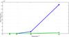 |
Fig. 9 The run times for the serial (blue) and parallel (green) versions of the multigrid code plotted against resolution. Each run time corresponds to the combined time for a 2D multigrid method calculation on the base of the domain and a 3D multigrid method calculation within the domain. |
5. Summary
In this paper we calculate linear MHS equilibria with an efficient numerical scheme based on the representation of NR99. The outline algorithm of this scheme is as follows:
-
Calculate the background equilibrium plasma plasma pressurepb and density ρb.
-
Prescribe Bz on the lower boundary and find the poloidal scalar potential P on this boundary by solving, using a multigrid method, the Poisson equation
 with
P defined on the side boundaries.
with
P defined on the side boundaries. -
Define the other boundary conditions for P, choose ξ < 1 and α, and solve, using a multigrid method,
![Mathematical equation: $$ [1-\xi(z)]\left(\frac{\partial^2P}{\partial x^2} +\frac{\partial^2P}{\partial y^2}\right) + \frac{\partial^2P}{\partial z^2} + \alpha^2 P = 0. $$](/articles/aa/full_html/2013/08/aa20458-12/aa20458-12-eq91.png)
-
Calculate the magnetic field by applying finite differences to
![Mathematical equation: $$ \vec{B} = \nabla\times[\nabla\times(P\hat{\vec{e}}_z) + \alpha P\hat{\vec{e}}_z]. $$](/articles/aa/full_html/2013/08/aa20458-12/aa20458-12-eq92.png)
-
Calculate the pressure directly using
-
Use finite differences to calculate the density with
The elegance of the NR99 formulation allows for an efficient numerical solution. We demonstrate the above scheme by calculating linear force-free and linear MHS equilibria. For the force-free case, we calculate an equilibrium with three footpoints and a null point. For the linear MHS case, we consider a region with two footpoints and investigate the effects of changing ξ. We consider profiles that cannot be treated, in the NR99 formalism, analytically and demonstrate how these can change the structure of the current distribution within the domain. We also show that the linear MHS equilibria are consistent with the Wilson effect for the size of the regions considered.
As well as demonstrating the scheme to be accurate, we show that the calculation time can be significantly reduced through parallelization on a GPU. This is achieved function by function and speed-ups of ×30 are realized. This result is significant as GPUs are inexpensive and readily available, unlike compute clusters and supercomputers. This fast and accurate scheme could be used for calculating equilibria in their own right or as input to MHD codes.
Acknowledgments
D.M. would like to thank the Royal Astronomical Society for financial support. J.M. acknowledges IDL support provided by STFC.
References
- Aulanier, G., Démoulin, P., Schmieder, B., Fang, C., & Tang, Y. H. 1998, Sol. Phys., 183, 369 [Google Scholar]
- Elman, H. C., Silvester, D. J., & Wathen, A. J. 2005, Finite Elements and Fast Iterative Solvers: with Applications in Incompressible Fluid Dynamics (Oxford University Press) [Google Scholar]
- Henning, B. S., & Cally, P. S. 2001, Sol. Phys., 201, 289 [NASA ADS] [CrossRef] [Google Scholar]
- Hood, A. W., Archontis, V., & MacTaggart, D. 2012, Sol. Phys., 278, 3 [NASA ADS] [CrossRef] [Google Scholar]
- Low, B. C. 1982, ApJ, 263, 952 [NASA ADS] [CrossRef] [Google Scholar]
- Low, B. C. 1991, ApJ, 370, 427 [NASA ADS] [CrossRef] [Google Scholar]
- Low, B. C. 1992, ApJ, 399, 300 [NASA ADS] [CrossRef] [Google Scholar]
- MacTaggart, D. 2011, A&A, 531, A108 [NASA ADS] [CrossRef] [EDP Sciences] [Google Scholar]
- McLaughlin, J. A., Verth, G.,Fedun, V., & Erdélyi, R. 2012, ApJ, 749, 30 [NASA ADS] [CrossRef] [Google Scholar]
- Neukirch, T., & Rastätter, L. 1999, A&A, 348, 1000 [NASA ADS] [Google Scholar]
- Petrie, G. J. D., & Neukirch, T. 2000, A&A, 356, 735 [NASA ADS] [Google Scholar]
- Régnier, S., Amari, T., & Canfield, R. C. 2005, A&A, 442, 345 [NASA ADS] [CrossRef] [EDP Sciences] [Google Scholar]
- Sanders, J., & Kandrot, E. 2011, CUDA by Example: An Introduction to General Purpose GPU Programming (Addison-Wesley) [Google Scholar]
- Spruit, H. C. 1976, Sol. Phys., 50, 269 [NASA ADS] [CrossRef] [Google Scholar]
All Figures
|
Fig. 1 Magnetic field lines of the linear force-free region are displayed in orange. A magnetogram of Bz is given at the base to indicate the positions of the sources. |
| In the text | |
|
Fig. 2 A map of | B |, within the range given on the scale, at z = 0.1. The null point is clearly highlighted between the two negative polarities. |
| In the text | |
|
Fig. 3 The profiles of ξ(z) from the cross-field current. |
| In the text | |
|
Fig. 4 Magnetic field lines for the MHS case with ξ1. The field lines are coloured with | ∇ × B |. |
| In the text | |
|
Fig. 5 Magnetic field lines for the MHS case with ξ2. The field lines are coloured with | ∇ × B |. |
| In the text | |
|
Fig. 6 An isosurface of | j| = 0.03 for the MHS solution with ξ1. |
| In the text | |
|
Fig. 7 An isosurface of | j| = 0.03 for the MHS solution with ξ2. |
| In the text | |
|
Fig. 8 The non-dimensional density along a diagonal cut through the domain at z = 0.46875. The two troughs correspond to the locations of the magnetic footpoints. This profile is for the linear MHS equilibrium with ξ2. |
| In the text | |
|
Fig. 9 The run times for the serial (blue) and parallel (green) versions of the multigrid code plotted against resolution. Each run time corresponds to the combined time for a 2D multigrid method calculation on the base of the domain and a 3D multigrid method calculation within the domain. |
| In the text | |
Current usage metrics show cumulative count of Article Views (full-text article views including HTML views, PDF and ePub downloads, according to the available data) and Abstracts Views on Vision4Press platform.
Data correspond to usage on the plateform after 2015. The current usage metrics is available 48-96 hours after online publication and is updated daily on week days.
Initial download of the metrics may take a while.