| Issue |
A&A
Volume 555, July 2013
|
|
|---|---|---|
| Article Number | A86 | |
| Number of page(s) | 7 | |
| Section | The Sun | |
| DOI | https://doi.org/10.1051/0004-6361/201321338 | |
| Published online | 04 July 2013 | |
Nonlinear Alfvén wave dynamics at a 2D magnetic null point: ponderomotive force
Department of Mathematics & Information SciencesNorthumbria
University,
Newcastle Upon Tyne,
NE1 8ST
UK
e-mail:
jonathan.thurgood@northumbria.ac.uk
Received:
21
February
2013
Accepted:
21
May
2013
Context. In the linear, β = 0 MHD regime, the transient properties of magnetohydrodynamic (MHD) waves in the vicinity of 2D null points are well known. The waves are decoupled and accumulate at predictable parts of the magnetic topology: fast waves accumulate at the null point; whereas Alfvén waves cannot cross the separatricies. However, in nonlinear MHD mode conversion can occur at regions of inhomogeneous Alfvén speed, suggesting that the decoupled nature of waves may not extend to the nonlinear regime.
Aims. We investigate the behaviour of low-amplitude Alfvén waves about a 2D magnetic null point in nonlinear, β = 0 MHD.
Methods. We numerically simulate the introduction of low-amplitude Alfvén waves into the vicinity of a magnetic null point using the nonlinear LARE2D code.
Results. Unlike in the linear regime, we find that the Alfvén wave sustains cospatial daughter disturbances, manifest in the transverse and longitudinal fluid velocity, owing to the action of nonlinear magnetic pressure gradients (viz. the ponderomotive force). These disturbances are dependent on the Alfvén wave and do not interact with the medium to excite magnetoacoustic waves, although the transverse daughter becomes focused at the null point. Additionally, an independently propagating fast magnetoacoustic wave is generated during the early stages, which transports some of the initial Alfvén wave energy towards the null point. Subsequently, despite undergoing dispersion and phase-mixing due to gradients in the Alfvén-speed profile (∇cA ≠ 0) there is no further nonlinear generation of fast waves.
Conclusions. We find that Alfvén waves at 2D cold null points behave largely as in the linear regime, however they sustain transverse and longitudinal disturbances – effects absent in the linear regime – due to nonlinear magnetic pressure gradients.
Key words: magnetohydrodynamics (MHD) / waves / Sun: corona / Sun: oscillations / Sun: magnetic topology / magnetic fields
© ESO, 2013
1. Introduction
Since the launch of solar satellites such as SDO, TRACE, Hinode, and STEREO, equipped with sufficiently high-resolution and high-cadence instrumentation, it has become established that magnetohydrodynamic (MHD) waves and oscillations are abundant throughout the coronal plasma (see, e.g., Nakariakov & Verwichte 2005; De Moortel 2005; Banerjee et al. 2007; Ruderman & Erdélyi 2009; Goosens et al. 2011; McLaughlin et al. 2012b). Consequently, it is clear that a well-developed theory of MHD waves is required to understand many ongoing coronal processes and dynamics. Due to the high degree of magnetic structuring in the atmospheric plasma, the medium in which these waves propagate is fundamentally inhomogeneous, leading to complex wave dynamics.
Magnetic null points, which are locations where magnetic induction (hence Alfvén speed) is zero, occur naturally in the corona as a consequence of the distribution of isolated magnetic flux sources on the photospheric surface, and are predicted by magnetic field extrapolations such as Brown & Priest (2001) and Beveridge et al. (2002). These null points are, like wave motions, prolific throughout the corona (Close et al. 2004; Longscope & Parnell 2009; and Régnier et al. 2008, give rough estimates of 1.0−4.0 × 10⁴ null points) and as such are a prime example of the extreme inhomogeneity that propagating MHD waves encounter in the corona. Null points have been implicated at the heart of many dynamic processes, such as in coronal mass ejections (the magnetic breakout model, e.g., Antichos 1998; Antichos et al. 1999) and in oscillatory reconnection (e.g., McLaughlin et al. 2009, 2012a). Study of MHD wave theory about null points therefore directly contributes to our understanding of wave propagation in realistic coronal plasmas.
The transient behaviour of linear waves about null points, and its consequences for solar physics, has been extensively studied (see the review by McLaughlin et al. 2011b). A series of investigations into linear MHD wave propagation in the vicinity of 2D β = 0 null points was carried out by McLaughlin & Hood (2004, 2005, 2006a). These studies give two key results for the linear regime: i) the fast and Alfvén waves accumulate at predictable regions of the null point topology, regardless of initial configuration; and ii) these wave modes remain distinct and decoupled, and do not interact.
Fast magnetoacoustic waves are focused towards the null point due to refraction, resulting in the accumulation of current density and ohmic heating at the null point. Linear 2D, β = 0 null points are thus predicted as locations of preferential heating due to passing fast magnetoacoustic waves. The Alfvén wave is found to accumulate along the separatricies, which it cannot cross.
Various studies that extend the 2D theory to β ≠ 0 and/or 3D (for example, McLaughlin & Hood 2006b; Galsgaard et al. 2003; McLaughlin et al. 2008; Thurgood & McLaughlin 2012) all confirm that these two key features carry over. These extensions also add further dynamics; for example, considering β ≠ 0 introduces the slow mode which interacts with the fast wave.
In nonlinear MHD, the nonlinear Lorentz force (sometimes referred to as the “ponderomotive force”) is known to facilitate interaction between the MHD modes in certain inhomogeneous scenarios. A large body of work regarding the ponderomotive effects of waves in various MHD scenarios has demonstrated that nonlinear Alfvén waves can generate magnetoacoustic waves as they propagate through regions of inhomogeneous Alfvén speed (such as, e.g., Nakariakov et al. 1997, 1998; Verwichte et al. 1999; Botha et al. 2000; Tsiklauri et al. 2001; McLaughlin et al. 2011a; Thurgood & McLaughlin 2013). The specific nature of ponderomotive mode conversion is dependent upon the gradients in the amplitude of the pulse and gradients in the Alfvén-speed profile. As such, in inhomogeneous magnetic topologies such as around null points, ponderomotive effects have the potential to make a significant impact upon the wave dynamics, energy transport, and dissipation.
The behaviour of the nonlinear fast wave at a 2D magnetic null point was investigated by McLaughlin et al. (2009). The authors found that, for sufficiently large driving amplitudes, magnetoacoustic shock waves develop, deform the null point and cause magnetic reconnection. The authors reported that in the nonlinear regime, some current can escape the null point, yet accumulation/heating still occurs (the shocks waves also heat the plasma). This process of oscillatory reconnection has been subsequently studied by Threlfall et al. (2012) and McLaughlin et al. (2012a).
Galsgaard et al. (2003) considered weakly nonlinear simulations of twisting motions about an azimuthally symmetric 2.5D null point and observed a small amount of current accumulation at the null point (relative to larger current accumulation along the spine/fan, which is associated with the Alfvén wave in the linear regime). The authors suggest that this is due to nonlinear mode conversion from the Alfvén to fast magnetoacoustic mode; however, their study did not consider the transient dynamics of waves and their interaction, but rather the current accumulation over time subject to an initial condition (i.e. they do not track the wave motions). Whilst the work of Thurgood & McLaughlin (2013) suggests that such nonlinear conversion could indeed be the explanation, it is unclear whether this is the case.
In this paper we address the question: how does the weakly nonlinear Alfvén wave behave in the vicinity of a 2D null point? To do so, we numerically solve the cold-plasma MHD equations to simulate the nonlinear wave dynamics at a null point where a pure linear Alfvén wave is driven at the boundary, i.e. initially we ensure there is no fast wave present. The paper is structured as follows. In Sect. 2.1 we describe the governing equations of the model, and in Sect. 2.2 we discuss the coordinate system used to distinguish between different MHD modes. In Sect. 3 we detail the numerical method and present the results of our simulations in Sect. 3.1. We discuss the nonlinear effects observed in our experiments in Sect. 4, and summarise in Sect. 5.
2. Mathematical model
2.1. Governing equations
We consider a plasma with dynamics described by ideal, 2.5D β = 0 MHD,
with translational invariance in the ẑ-direction; thus
∂/∂z = 0. The governing nonlinear
MHD equations are ![\begin{eqnarray} \label{MHDeqns} \rho\left[\frac{\partial\vec{v}}{\partial t}+(\vec{v}\cdot\mathbf{\nabla})\vec{v}\right]&=& \left(\frac{\mathbf{\nabla}\times\vec{B}}{\mu} \right)\times\vec{B}\quad \nonumber \\ \frac{\partial\vec{B}}{\partial t}&=&\mathbf{\nabla}\times(\vec{v}\times\vec{B})\quad\nonumber\\ \frac{\partial\rho}{\partial t}&=& -\mathbf{\nabla}\cdot(\rho\vec{v}) \quad \end{eqnarray}](/articles/aa/full_html/2013/07/aa21338-13/aa21338-13-eq7.png) (1)where
the standard MHD notation applies: v is plasma velocity, ρ
is density, B is the magnetic field/induction,
γ = 5/3 is the adiabatic index, and
μ is the magnetic permeability. We consider an equilibrium state of
ρ = ρ0, (where
ρ0 is constant), v = 0 and
equilibrium magnetic field B = B0. Finite
perturbations are considered in the form
ρ = ρ0 + ρ1(r,t),
v = 0 + v(r,t) and
B = B0 + b(r,t)
and a subsequent nondimensionalisation using the substitution
(1)where
the standard MHD notation applies: v is plasma velocity, ρ
is density, B is the magnetic field/induction,
γ = 5/3 is the adiabatic index, and
μ is the magnetic permeability. We consider an equilibrium state of
ρ = ρ0, (where
ρ0 is constant), v = 0 and
equilibrium magnetic field B = B0. Finite
perturbations are considered in the form
ρ = ρ0 + ρ1(r,t),
v = 0 + v(r,t) and
B = B0 + b(r,t)
and a subsequent nondimensionalisation using the substitution
 ,∇ = ∇∗/L,
 ,
b = B0b∗,
,
b = B0b∗,
 ,
,
 and
and
 is performed, with
the additional choices
is performed, with
the additional choices  and
and
 /
/ .
The resulting nondimensionalised, governing equations of the perturbed system are
.
The resulting nondimensionalised, governing equations of the perturbed system are
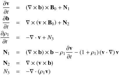 (2)where
terms Ni are the nonlinear components. The star
indices have been dropped, henceforth all equations are presented in a nondimensional
form. The equations are merged into one governing PDE
(2)where
terms Ni are the nonlinear components. The star
indices have been dropped, henceforth all equations are presented in a nondimensional
form. The equations are merged into one governing PDE ![\begin{eqnarray} \label{eqn:governingPDE} \frac{\partial^2 \vec{v}}{\partial t^2}&=&\left\lbrace\mathbf{\nabla}\times\left[\mathbf{\nabla}\times\left(\vec{v}\times\vec{B}_0\right)\right]\right\rbrace\times\vec{B}_0 + \vec{N} \nonumber \\ \vec{N}&=&\left\lbrace\mathbf{\nabla}\times\left[\mathbf{\nabla}\times\left(\vec{v}\times\vec{b}\right)\right]\right\rbrace\times \left(\vec{B}_0+\vec{b}\right) \nonumber \\ & & +\left(\nabla\times\vec{b}\right)\times \left[\nabla\times\left(\vec{v}\times\vec{B}_{0}\right)\right] \nonumber \\ & & + \left(\mathbf{\nabla}\cdot\vec{v} - \vec{v} \cdot \mathbf{\nabla}\right)\left(\mathbf{\nabla}\times\vec{b}\right)\times\vec{B}_0 \nonumber\\ & & - \rho_1 \left\lbrace\mathbf{\nabla}\times\left[\mathbf{\nabla}\times\left(\vec{v}\times\vec{B}_0\right)\right]\right\rbrace\times\vec{B}_0 \nonumber \\ & & - \left[ \left(\mathbf{\nabla}\times\vec{b}\right)\times\vec{B}_0 \cdot\mathbf{\nabla}\right] \vec{v} . \end{eqnarray}](/articles/aa/full_html/2013/07/aa21338-13/aa21338-13-eq32.png) (3)The
first term describes the linear regime of the system and the terms N are the
nonlinear terms, displayed here to the second order for brevity (N.B. our solution solves
the full system of equations, with all nonlinear terms, see Sect. 3 and Arber et al. 2001).
(3)The
first term describes the linear regime of the system and the terms N are the
nonlinear terms, displayed here to the second order for brevity (N.B. our solution solves
the full system of equations, with all nonlinear terms, see Sect. 3 and Arber et al. 2001).
2.2. Isolating MHD modes
Thurgood & McLaughlin (2012) developed a magnetic-flux-based coordinate system that allows the decomposition of MHD waves into constituent modes and the construction of initial conditions that correspond to single linear modes of oscillation. This approach is suitable for any MHD scenario that is capable of sustaining true Alfvén waves – i.e. where the equilibrium configuration permits some invariant direction (see their Sect. 2.3.1).
The projected perturbations corresponding to the wave modes according to this coordinate
system are 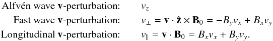 Perturbations
in the invariant direction elicit magnetic tension only and thus correspond to the Alfvén
wave. Perturbations in the direction transverse to both the equilibrium field and the
invariant direction (here the xy-plane) correspond to the fast wave, and
perturbations in the longitudinal direction are static as there is no longitudinal force
to transport the disturbance in our β = 0 scenario (and would correspond
to the slow wave in β ≠ 0).
Perturbations
in the invariant direction elicit magnetic tension only and thus correspond to the Alfvén
wave. Perturbations in the direction transverse to both the equilibrium field and the
invariant direction (here the xy-plane) correspond to the fast wave, and
perturbations in the longitudinal direction are static as there is no longitudinal force
to transport the disturbance in our β = 0 scenario (and would correspond
to the slow wave in β ≠ 0).
Note that this corresponds to the coordinate system used in McLaughlin & Hood (2004) which is a specific implementation of the flux-based coordinate system appropriate for 2D magnetic null points.
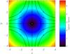 |
Fig. 1 Indicative lines of the equilibrium magnetic field structure
B0 (black lines) and contours of the Alfvén-speed profile
|
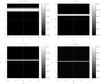 |
Fig. 2 The evolution of vz (the Alfvén wave) over time. The Alfvén wave propagates along fieldlines at the Alfvén speed, hence we see a narrowing planar pulse propagating towards the y = 0 separatrix (the separatricies are marked by dashed white lines). |
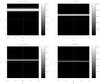 |
Fig. 3 The longitudinal component v∥ over time. We find that the ponderomotive force of the propagating Alfvén wave (position marked by green lines) sustains a cospatial disturbance in velocity along the background magnetic field. This longitudinal daughter disturbance is a ponderomotive effect which in this case does not facilitate any conversion to the slow mode. |
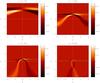 |
Fig. 4 The evolution of v⊥ over time. We find two pronounced nonlinear effects: a transverse daughter disturbance which is cospatial to the Alfvén wave (indicated by dashed green lines) and an independently propagating fast wave. |
3. Numerical simulation
We solve the full set of the nonlinear, nondimensionalised MHD Eq. (2) with the (nondimensionalised) equilibrium
magnetic field ![\begin{equation} \vec{B}_{0}=\left[x,-y, 0\right] \label{eqn:2D_null_point} \end{equation}](/articles/aa/full_html/2013/07/aa21338-13/aa21338-13-eq42.png) (4)using
the fully nonlinear, shock-capturing LARE2D code (Arber et al. 2001). Equation (4)
corresponds to a 2D null point with two key topological features, the null point itself
where magnetic induction is zero at the origin, and the separatrices at
x = 0 and y = 0 lines (see Fig. 1 and McLaughlin et al. 2011b). We
drive planar, sinusoidal pulses in vz and
bz at the upper y-boundary
to introduce a linear Alfvén wave as per Sect. 2.2. To
do so we drive
(4)using
the fully nonlinear, shock-capturing LARE2D code (Arber et al. 2001). Equation (4)
corresponds to a 2D null point with two key topological features, the null point itself
where magnetic induction is zero at the origin, and the separatrices at
x = 0 and y = 0 lines (see Fig. 1 and McLaughlin et al. 2011b). We
drive planar, sinusoidal pulses in vz and
bz at the upper y-boundary
to introduce a linear Alfvén wave as per Sect. 2.2. To
do so we drive  (5)for
0 ≤ t ≤ 0.5, and we consider a driving amplitude
A = 0.001. This amplitude is small with respect to the characteristic
velocity of the non-dimensionalisation used in Sect. 2.1 (, i.e. a typical
Alfvén crossing time over the length scale of interest) and thus we consider the weakly
nonlinear scenario. Simple zero-gradient conditions are employed on the other boundaries,
and the simulations are performed over the domain
x ∈ [−4,4],
y ∈ [−4,4] with 2400 × 2400 grid points.
(5)for
0 ≤ t ≤ 0.5, and we consider a driving amplitude
A = 0.001. This amplitude is small with respect to the characteristic
velocity of the non-dimensionalisation used in Sect. 2.1 (, i.e. a typical
Alfvén crossing time over the length scale of interest) and thus we consider the weakly
nonlinear scenario. Simple zero-gradient conditions are employed on the other boundaries,
and the simulations are performed over the domain
x ∈ [−4,4],
y ∈ [−4,4] with 2400 × 2400 grid points.
3.1. Results
In Fig. 2, we plot the propagating Alfvén wave in
the velocity component vz. We have computed
the bz perturbation which shows a
qualitatively identical result. It is known that the linear Alfvén wave propagates along
the magnetic field lines at the Alfvén speed cA (here
 ),
causing spreading of pulses along field lines and is unable to cross the separatricies
(McLaughlin & Hood 2004). Given that our
driving imposes a planar profile, this spreading effect is not obvious in our simulation,
instead we see the planar pulse that propagates towards the y = 0
separatrix at a speed which is equivalent to the Alfvén speed evaluated at
x = 0. It cannot cross the separatrix, as
cA|x = 0 → 0 as
y → 0, and it accumulates nearby with ever increasing gradients, hence
resistive dissipation will eventually become an important consideration (McLaughlin
& Hood 2004). Thus,
vz behaves as in the linear regime.
),
causing spreading of pulses along field lines and is unable to cross the separatricies
(McLaughlin & Hood 2004). Given that our
driving imposes a planar profile, this spreading effect is not obvious in our simulation,
instead we see the planar pulse that propagates towards the y = 0
separatrix at a speed which is equivalent to the Alfvén speed evaluated at
x = 0. It cannot cross the separatrix, as
cA|x = 0 → 0 as
y → 0, and it accumulates nearby with ever increasing gradients, hence
resistive dissipation will eventually become an important consideration (McLaughlin
& Hood 2004). Thus,
vz behaves as in the linear regime.
We now consider the other orthogonal velocity components (v⊥
and v∥) which remain zero throughout linear simulations, to
investigate possible nonlinear effects. We first consider the longitudinal velocity
component v∥, shown in Fig. 3. Here, we find a nonlinear disturbance of
 ,
which is cospatial to the Alfvén wave pulse in time (the front and rear position of the
Alfvén pulse is marked by green lines). The pulse appears similar in profile to that of
the Alfvén wave, however is more compressed and steep, i.e. the profile is approximately
as a squared sine wave, whereas vz is
sinusoidal. This disturbance is not an independently propagating wave (in
β = 0 such motion is prohibited), but a direct consequence of the
longitudinal component of the ponderomotive force, which is induced, sustained and carried
by the propagating Alfvén wave. This is the specific manifestation of the longitudinal
daughter disturbance, a general feature of nonlinear Alfvén waves and a common
manifestation of the ponderomotive force (see Thurgood & McLaughlin 2013 for a detailed discussion).
,
which is cospatial to the Alfvén wave pulse in time (the front and rear position of the
Alfvén pulse is marked by green lines). The pulse appears similar in profile to that of
the Alfvén wave, however is more compressed and steep, i.e. the profile is approximately
as a squared sine wave, whereas vz is
sinusoidal. This disturbance is not an independently propagating wave (in
β = 0 such motion is prohibited), but a direct consequence of the
longitudinal component of the ponderomotive force, which is induced, sustained and carried
by the propagating Alfvén wave. This is the specific manifestation of the longitudinal
daughter disturbance, a general feature of nonlinear Alfvén waves and a common
manifestation of the ponderomotive force (see Thurgood & McLaughlin 2013 for a detailed discussion).
Now we consider the fast-mode velocity component v⊥, shown in
Fig. 4, which consists of two features: a wave that
propagates independently of the Alfvén wave and a cospatial disturbance, both nonlinear of
order .
The independently propagating wave is generated during the driving stage of the
simulation, and propagates with the transient characteristics of a linear fast wave at a
single null point, namely that it undergoes refraction due to the Alfvén-speed profile,
crosses the separatricies and accumulates at the null point. Hence, driving a linear
Alfvén wave according to Eq. (5) has
nonlinearly excited a fast wave.
We also find a disturbance in v⊥ which does not appear to correspond to a fast wave (qualitatively, in terms of transient behaviour), and is cospatial to the Alfvén wave pulse (again, the position of which is shown by the green envelope in Fig. 4). This is the transverse daughter disturbance, detailed for general MHD in Thurgood & McLaughlin (2013). This disturbance is not an independently propagating wave. Within the cospatial region, the disturbance becomes increasing focused towards the separatrix and ultimately to the vicinity of the null point.
4. Nonlinear effects
Here, due to the choice of small driving amplitude A,
vz behaves as in the linear regime (Fig.
2). Whilst the choice of a low driving amplitude
makes the nonlinear effects small, it is nonetheless sufficient to demonstrate in what ways
the (shock-free) nonlinear system differs from the linear, in particular its interaction
with the transverse and longitudinal fluid variables and between differing modes of
oscillation. Here we see two types of nonlinear effects which are absent in the linear study
of McLaughlin & Hood (2004), both of which
are generated or sustained at  :
and
:
and
4.1. Daughter disturbances
In the simulations, we observe disturbances in v⊥ and
v∥ which develop immediately and remain cospatial to the
wave observed in vz throughout the
simulations. The Alfvén wave exerts a nonlinear magnetic pressure gradient (viz.
ponderomotive force) upon the medium, resulting in these transverse and longitudinal
daughter disturbances. Thurgood & McLaughlin (2013) discuss the MHD-ponderomotive effects of Alfvén waves in detail, and show
that such daughters will be sustained anywhere there are non-zero gradients in the pulse
amplitude relative to the equilibrium magnetic field. At any given instant, the
ponderomotive force of an Alfvén wave manifest in ẑ across and along the
field is (Thurgood & McLaughlin 2013, Sect.
3, Eqs. (12)−(13)) 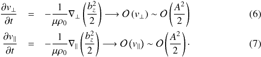 Here,
∇⊥ ≡ ẑ × B0·∇ and
∇∥ ≡ B0·∇ (these terms are the gradients transverse
and longitudinal relative to the equilibrium magnetic field) and
Here,
∇⊥ ≡ ẑ × B0·∇ and
∇∥ ≡ B0·∇ (these terms are the gradients transverse
and longitudinal relative to the equilibrium magnetic field) and
 . Where the net
ponderomotive force over a wave period is non-zero, excitation of magnetoacoustic modes
occurs. Where the action of the force of the leading pulse edge is consistently nullified
by the trailing edge, disturbances arise in the transverse and longitudinal
fluid-variables that do not excite wave motions but remain confined to a region cospatial
to the Alfvén wave, referred to as the ponderomotive envelope (see discussion of, e.g.,
“ponderomotive wings” in Verwichte et al. 1999; and
“daughter disturbances” in Thurgood & McLaughlin 2013).
. Where the net
ponderomotive force over a wave period is non-zero, excitation of magnetoacoustic modes
occurs. Where the action of the force of the leading pulse edge is consistently nullified
by the trailing edge, disturbances arise in the transverse and longitudinal
fluid-variables that do not excite wave motions but remain confined to a region cospatial
to the Alfvén wave, referred to as the ponderomotive envelope (see discussion of, e.g.,
“ponderomotive wings” in Verwichte et al. 1999; and
“daughter disturbances” in Thurgood & McLaughlin 2013).
In Sect. 3, the spatial distribution of the
amplitude of these two disturbances differs; the longitudinal daughter
(v∥) varies uniformly in ŷ with a similar
profile to that of the Alfvén wave in vz (as
the disturbance is generated at amplitude A2, the profile is
more akin to that of the squared sine wave, i.e. more compressed and steep). However, the
transverse daughter (v⊥) varies in both
 and ŷ, is of opposite sign either side of the x = 0
separatrix, and appears to become increasingly focused towards the x = 0
separatrix as time evolves. By considering (6) and (7) with the equilibrium
field (4) and given that in the simulation
the pulse remains planar in
(i.e. has ∂/∂x = 0 throughout), the
transverse and longitudinal nonlinear magnetic pressure gradients (ponderomotive force)
assume profiles such that
and ŷ, is of opposite sign either side of the x = 0
separatrix, and appears to become increasingly focused towards the x = 0
separatrix as time evolves. By considering (6) and (7) with the equilibrium
field (4) and given that in the simulation
the pulse remains planar in
(i.e. has ∂/∂x = 0 throughout), the
transverse and longitudinal nonlinear magnetic pressure gradients (ponderomotive force)
assume profiles such that 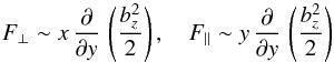 (8)where
we know, from the numerical results where the leading edge propagates slower than the
trailing (hence length scales decrease and gradients grow), that the derivative value
becomes larger in time and the pulse profile changes in y, but that in
x does not. Transversely, within the ponderomotive envelope, there is
an applied pressure gradient which overall becomes stronger as the Alfvén wave tends
towards the y = 0 separatrix (as the gradient increases) yet maintains
the same profile proportional to | x | throughout, with zero magnetic
pressure along x = 0. In the simulation, we see that the transverse
daughter becomes increasingly focused towards x = 0. Hence, a possible
explanation is that the applied magnetic pressure gradient acts to accelerate the fluid
within the envelope towards x = 0. Longitudinally, as the leading edge of
the Alfvén wave undergoes steepening the derivative value will be larger at the lead than
that towards the trailing edge, however the value of y is smaller. Since
in the simulations we see no static perturbations in v∥ or
b∥, the net force must be zero and thus the change in
y must be proportional to the increasing steepness of the leading edge
throughout the simulation (this is intuitive, as net speed of the pulse in the
ŷ-direction also decreases proportional to y). Hence, we
are confident that the observed phenomena are ponderomotive daughter disturbances, as they
are generated at a nonlinear order and are consistent with Eq. (8).
(8)where
we know, from the numerical results where the leading edge propagates slower than the
trailing (hence length scales decrease and gradients grow), that the derivative value
becomes larger in time and the pulse profile changes in y, but that in
x does not. Transversely, within the ponderomotive envelope, there is
an applied pressure gradient which overall becomes stronger as the Alfvén wave tends
towards the y = 0 separatrix (as the gradient increases) yet maintains
the same profile proportional to | x | throughout, with zero magnetic
pressure along x = 0. In the simulation, we see that the transverse
daughter becomes increasingly focused towards x = 0. Hence, a possible
explanation is that the applied magnetic pressure gradient acts to accelerate the fluid
within the envelope towards x = 0. Longitudinally, as the leading edge of
the Alfvén wave undergoes steepening the derivative value will be larger at the lead than
that towards the trailing edge, however the value of y is smaller. Since
in the simulations we see no static perturbations in v∥ or
b∥, the net force must be zero and thus the change in
y must be proportional to the increasing steepness of the leading edge
throughout the simulation (this is intuitive, as net speed of the pulse in the
ŷ-direction also decreases proportional to y). Hence, we
are confident that the observed phenomena are ponderomotive daughter disturbances, as they
are generated at a nonlinear order and are consistent with Eq. (8).
4.2. Independently propagating fast wave
In Sect. 3 we have seen that a wave in v⊥ is generated during the driving phase (0 ≤ t < 0.5). This wave subsequently propagates with all of the transient features of a linear fast magnetoacoustic wave (refracting about the Alfvén speed profile and accumulating at the null point). As the nonlinear magnetic pressure is the only facilitator of coupling between vz and v⊥ in cold, 2.5D MHD systems, the generation of such a wave is due to the exertion of a transverse ponderomotive force (Eq. (6)) such that the net force over the period is non-zero. After the driving phase, no further excitation of fast waves occurs, thus the net ponderomotive force must be zero (and thus is only manifest in the aforementioned daughters). Hence, after this driving period gradients in the trailing edge nullify the fluid acceleration caused by the gradients in the leading edge.
The value of the net ponderomotive force can only change if the pulse geometry is altered. This requires a change in the Alfvén speed. Here, gradients in the Alfvén speed are non-zero
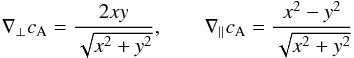 generally
permitting such changes in the pulse geometry (i.e. our system is inhomogeneous). However
since we impose a planar profile, the effective speed of the wave is
cA|x = 0 = y,
and its derivative in the direction of propagation is constant. Thus, as the Alfvén wave
propagates its geometry is not altered such that there should be a change from a non-zero
to zero net ponderomotive force.
generally
permitting such changes in the pulse geometry (i.e. our system is inhomogeneous). However
since we impose a planar profile, the effective speed of the wave is
cA|x = 0 = y,
and its derivative in the direction of propagation is constant. Thus, as the Alfvén wave
propagates its geometry is not altered such that there should be a change from a non-zero
to zero net ponderomotive force.
This raises the question that, since the net force cannot change, why do we observe the generation of fast waves only during the driving phase, rather than continuously? There are two possible explanations
-
(i)
the net force is initially non-zero and remains so, i.e. there is a physical mechanism which suppresses the further generation of independently propagating fast waves.
-
(ii)
the net force is actually zero, thus no ponderomotive excitation of the fast mode should occur. The excitation of the fast wave is a consequence of linearly driving a nonlinear system.
4.2.1. Physical effect
If the net-force of the wave is always non-zero, in the absence of continuous fast wave generation a mechanism must act to oppose further wave excitation. Botha et al. (2000) considered the case of a harmonic Alfvén wave propagating in a homogeneous field stratified by a transverse density profile. They reported that the transverse gradients caused the nonlinear excitation of fast waves. However, these waves eventually saturated and did not continue to develop in time. This saturation was also later reported to occur for pulse-type Alfvén waves in the same equilibrium set-up by Tsiklauri et al. (2001). Botha et al. (2000) proposed that the saturation occurs due to wave interference between the generated fast waves. It is possible that in our system a level of saturation sufficient to oppose further mode conversion is reached so rapidly that only a single independent fast wave is generated.
4.2.2. Mathematical artefact
If the net ponderomotive force is zero throughout, then the independent fast wave has been introduced as a mathematical consequence of our driving condition. We have used the driving condition (5) so we can directly compare our nonlinear experiment to the linear results of McLaughlin & Hood (2004). However, in nonlinear MHD, driving the ẑ-components of the fluid variables and holding the transverse and longitudinal components at zero corresponds to an Alfvén wave with no instantaneous ponderomotive force. The driven Alfvén wave subsequently enters an inhomogeneous region which alters the pulse profile and contributes to the nonlinear magnetic pressure perturbation, unopposed by other factors (which are specified as zero). Thus a non-zero ponderomotive force acts across the field, resulting in the fast wave, and along the field, resulting in a static longitudinal perturbation, as β = 0 (this is subsequently removed by our boundary post-driving boundary conditions, hence absent from our discussion in Sect. 3).
If this is indeed the case, then physically boundary condition (5) is inappropriate as it corresponds to an incoming wave with no ponderomotive daughters, and hence no ponderomotive force. At the bare minimum, longitudinal daughters are present for Alfvén wave pulses in straight-field, homogeneous MHD (see Verwichte et al. 1999). From the perspective of wave-stability the driving conditions used are entirely appropriate in the linear regime, as they correspond to a pure linear Alfvén wave (i.e. a wave driven solely by magnetic tension, as per Alfvén 1942) that does not interact with other modes of oscillation (see Parker 1991). This can be be confirmed by considering Eq. (3) with N = 0 in the flux-based coordinate system, which yields three separate and decoupled equations for invariant, transverse and longitudinal variables, i.e. for the Alfvén, fast and (absent) slow modes of oscillation. As perturbations in ẑ do not elicit responses in other directions in the linear regime, such a wave could be considered linearly stable. However, in the full nonlinear system, disturbances to vz do not exist independently to perturbations in v⊥ and v∥ due to the action of the ponderomotive force. The driving conditions still successfully introduce an Alfvén wave (in the nonlinear regime the motion of an Alfvén wave is still primarily due to linear magnetic tension), yet specify values of transverse and longitudinal fluid variables that are inconsistent with those specified by the equations for a single Alfvén wave (these values should correspond to those implied by Eqs. (6) and (7)).
In the absence of a physical saturation mechanism such as that described in Sect. 4.2.1, the independent fast wave is a consequence of linearly driving a nonlinear system; the solution is mathematically consistent with the equations, which introduce a small fast wave via a boundary-ponderomotive effect.
5. Summary
In this paper we have addressed the question, how does the weakly nonlinear Alfvén wave behave in the vicinity of a 2D null point? The null point topology (4) and equilibrium variables considered are identical to those considered in the linear study of McLaughlin & Hood (2004), as is the method for introducing the Alfvén wave (i.e. driving the ẑ-components of the fluid variables). Thus, we can directly compare the behaviour of the waves in the linear and nonlinear regimes. Our three main results are that
-
(i)
In vz, the wave propagates along fieldlines at the background Alfvén speed, cA, accumulating at the separatricies. The wave does not steepen to form a shock (hence, we refer to our choice of A as low amplitude).
-
(ii)
The Alfvén wave sustains cospatial, nonlinear disturbances that have transverse (v⊥, Fig. 4) and longitudinal (v∥, Fig. 3) manifestations – phenomena not reported before in null point simulations.
-
(iii)
During the driving phase, a wave develops in v⊥ and subsequently propagates independently of the Alfvén wave. It propagates with the transient properties of a linear fast wave, crossing separatricies and accumulating at the null point.
The longitudinal daughter, sustained by the Alfvén wave, appears to have no real impact upon the medium. The transverse daughter appears to be focused towards x = 0 separatrix, and thus the null point as the Alfvén wave carries it towards y = 0. Since the amplitude here is small, such an effect has very little impact on energy transport and dissipation in the vicinity of the null, however the effect has the potential to be significant for larger amplitude Alfvén waves.
A key feature of linear 2D nulls is that the Alfvén wave and magnetoacoustic modes are decoupled, and that Alfvén wave energy accumulates along the separatricies and not at the null. However, in the nonlinear case we observe the ponderomotive excitation of a fast magnetoacoustic wave which refracts about and eventually accumulates at the null point. Thus, unlike in 2D, some of the Alfvén wave’s energy is focused at the null point by the fast wave.
After the initial generation of the fast magnetoacoustic wave, we note that no further magnetoacoustic waves are generated, despite the fact that the pulse is travelling through an inhomogeneous region – undergoing longitudinal dispersion (∇∥ cA ≠ 0) and phase mixing (∇⊥ cA ≠ 0). The analysis of Thurgood & McLaughlin (2013) demonstrated that when a pulse propagates through an inhomogeneous medium, mode conversion can occur, but that it is dependent on the specific scenario (e.g., the phase-mixing experiment of Nakariakov et al. 1997). As no conversion occurs in our experiment after the initial excitation, ∇ cA in the vicinity of our 2D null point must not be sufficiently steep or sharp enough to further excite magnetoacoustic waves. This suggests that ponderomotive mode conversion due to inhomogeneity will only routinely occur where this profile is sharp or discontinuous.
Acknowledgments
The authors acknowledge IDL support provided by STFC. J.O.T. acknowledges travel support provided by the RAS and the IMA, and a Ph.D. scholarship provided by Northumbria University. The computational work for this paper was carried out on the joint STFC and SFC (SRIF) funded cluster at the University of St Andrews (Scotland, UK).
References
- Alfvén, H. 1942, Nature, 150, 405 [NASA ADS] [CrossRef] [Google Scholar]
- Antiochos, S. K. 1998, ApJ, 502, L181 [NASA ADS] [CrossRef] [Google Scholar]
- Antiochos, S. K., DeVore, C. R., & Klimchuk, J. A. 1999, ApJ, 510, 485 [Google Scholar]
- Arber, T. D., Longbottom, A. W., Gerrard, C. L., & Milne, A. M. 2001, J. Computat. Phys., 171, 151 [Google Scholar]
- Banerjee, D., Erdélyi, R., Oliver, R., & O’Shea, E. 2007, Sol. Phys., 246, 3 [NASA ADS] [CrossRef] [Google Scholar]
- Beveridge, C., Priest, E. R., & Brown, D. S. 2002, Sol. Phys., 209, 333 [NASA ADS] [CrossRef] [Google Scholar]
- Botha, G. J. J., Arber, T. D., Nakariakov, V. M., & Keenan, F. P. 2000, A&A, 363, 1186 [NASA ADS] [Google Scholar]
- Brown, D. S., & Priest, E. R. 2001, A&A, 367, 339 [NASA ADS] [CrossRef] [EDP Sciences] [Google Scholar]
- Close, R. M., Parnell, C. E., & Priest, E. R. 2004, Sol. Phys., 225, 21 [NASA ADS] [CrossRef] [Google Scholar]
- De Moortel, I. 2005, Roy. Soc. London Philosoph. Trans. Ser. A, 363, 2743 [Google Scholar]
- Galsgaard, K., Priest, E. R., & Titov, V. S. 2003, J. Geophys. Res., 108 [Google Scholar]
- Goossens, M., Erdélyi, R., & Ruderman, M. S. 2011, Space Sci. Rev., 158, 289 [NASA ADS] [CrossRef] [Google Scholar]
- Longcope, D. W., & Parnell, C. E. 2009, Sol. Phys., 254, 51 [NASA ADS] [CrossRef] [Google Scholar]
- McLaughlin, J. A., & Hood, A. W. 2004, A&A, 420, 1129 [NASA ADS] [CrossRef] [EDP Sciences] [Google Scholar]
- McLaughlin, J. A., & Hood, A. W. 2005, A&A, 435, 313 [NASA ADS] [CrossRef] [EDP Sciences] [Google Scholar]
- McLaughlin, J. A., & Hood, A. W. 2006a, A&A, 452, 603 [NASA ADS] [CrossRef] [EDP Sciences] [Google Scholar]
- McLaughlin, J. A., & Hood, A. W. 2006b, A&A, 459, 641 [NASA ADS] [CrossRef] [EDP Sciences] [Google Scholar]
- McLaughlin, J. A., Ferguson, J. S. L., & Hood, A. W. 2008, Sol. Phys., 251, 563 [NASA ADS] [CrossRef] [Google Scholar]
- McLaughlin, J. A., De Moortel, I., Hood, A. W., & Brady, C. S. 2009, A&A, 493, 227 [NASA ADS] [CrossRef] [EDP Sciences] [Google Scholar]
- McLaughlin, J. A., De Moortel, I., & Hood, A. W. 2011a, A&A, 527, A149 [NASA ADS] [CrossRef] [EDP Sciences] [Google Scholar]
- McLaughlin, J. A., Hood, A. W., & De Moortel, I. 2011b, Space Sci. Rev., 158, 205 [NASA ADS] [CrossRef] [Google Scholar]
- McLaughlin, J. A., Thurgood, J. O., & MacTaggart, D. 2012a, A&A, 548, A98 [NASA ADS] [CrossRef] [EDP Sciences] [Google Scholar]
- McLaughlin, J. A., Verth, G., Fedun, V., & Erdélyi, R. 2012b, ApJ, 749, 30 [NASA ADS] [CrossRef] [Google Scholar]
- Nakariakov, V. M., & Verwichte, E. O. 2005, Liv. Rev. Sol. Phys., 2, 3 [Google Scholar]
- Nakariakov, V. M., Roberts, B., & Murawski, K. 1997, Sol. Phys., 175, 93 [NASA ADS] [CrossRef] [Google Scholar]
- Nakariakov, V. M., Roberts, B., & Murawski, K. 1998, A&A, 332, 795 [NASA ADS] [Google Scholar]
- Parker, E. N. 1991, ApJ, 376, 355 [NASA ADS] [CrossRef] [Google Scholar]
- Régnier, S., Parnell, C. E., & Haynes, A. L. 2008, A&A, 484, L47 [NASA ADS] [CrossRef] [EDP Sciences] [Google Scholar]
- Ruderman, M. S., & Erdélyi, R. 2009, Space Sci. Rev., 149, 199 [NASA ADS] [CrossRef] [Google Scholar]
- Threlfall, J., Parnell, C. E., De Moortel, I., McClements, K. G., & Arber, T. D. 2012, A&A, 544, A24 [NASA ADS] [CrossRef] [EDP Sciences] [Google Scholar]
- Thurgood, J. O., & McLaughlin, J. A. 2012, A&A, 545, A9 [NASA ADS] [CrossRef] [EDP Sciences] [Google Scholar]
- Thurgood, J. O., & McLaughlin, J. A. 2013, Sol. Phys., in press, DOI: 10.1007/s11207-013-0298-4 [Google Scholar]
- Tsiklauri, D., Arber, T. D., & Nakariakov, V. M. 2001, A&A, 379, 1098 [NASA ADS] [CrossRef] [EDP Sciences] [Google Scholar]
- Verwichte, E., Nakariakov, V. M., & Longbottom, A. W. 1999, J. Plasma Phys., 62, 219 [NASA ADS] [CrossRef] [Google Scholar]
All Figures
|
Fig. 1 Indicative lines of the equilibrium magnetic field structure
B0 (black lines) and contours of the Alfvén-speed profile
|
| In the text | |
|
Fig. 2 The evolution of vz (the Alfvén wave) over time. The Alfvén wave propagates along fieldlines at the Alfvén speed, hence we see a narrowing planar pulse propagating towards the y = 0 separatrix (the separatricies are marked by dashed white lines). |
| In the text | |
|
Fig. 3 The longitudinal component v∥ over time. We find that the ponderomotive force of the propagating Alfvén wave (position marked by green lines) sustains a cospatial disturbance in velocity along the background magnetic field. This longitudinal daughter disturbance is a ponderomotive effect which in this case does not facilitate any conversion to the slow mode. |
| In the text | |
|
Fig. 4 The evolution of v⊥ over time. We find two pronounced nonlinear effects: a transverse daughter disturbance which is cospatial to the Alfvén wave (indicated by dashed green lines) and an independently propagating fast wave. |
| In the text | |
Current usage metrics show cumulative count of Article Views (full-text article views including HTML views, PDF and ePub downloads, according to the available data) and Abstracts Views on Vision4Press platform.
Data correspond to usage on the plateform after 2015. The current usage metrics is available 48-96 hours after online publication and is updated daily on week days.
Initial download of the metrics may take a while.