| Issue |
A&A
Volume 555, July 2013
|
|
|---|---|---|
| Article Number | A139 | |
| Number of page(s) | 11 | |
| Section | The Sun | |
| DOI | https://doi.org/10.1051/0004-6361/201220830 | |
| Published online | 12 July 2013 | |
High-rigidity Forbush decreases: due to CMEs or shocks?⋆
1
Indian Institute of Science Education and Research,
Sai Trinity Building, Pashan,
411 021
Pune, India
2
Tata Institute of Fundamental Research,
Homi Bhabha Road, 400 005
Mumbai,
India
3
The GRAPES–3 Experiment, Cosmic Ray Laboratory,
Raj Bhavan, 643 001
Ooty,
India
4
Graduate School of Science, Osaka City University,
558-8585
Osaka,
Japan
5
National Astronomical Observatory of Japan, CfCA,
181-8588
Tokyo,
Japan
Received:
2
December
2012
Accepted:
17
April
2013
Abstract
Aims. We seek to identify the primary agents causing Forbush decreases (FDs) in high-rigidity cosmic rays observed from the Earth. In particular, we ask if these FDs are caused mainly by coronal mass ejections (CMEs) from the Sun that are directed towards the Earth, or by their associated shocks.
Methods. We used the muon data at cutoff rigidities ranging from 14 to 24 GV from the GRAPES-3 tracking muon telescope to identify FD events. We selected those FD events that have a reasonably clean profile, and can be reasonably well associated with an Earth-directed CME and its associated shock. We employed two models: one that considers the CME as the sole cause of the FD (the CME-only model) and one that considers the shock as the only agent causing the FD (the shock-only model). We used an extensive set of observationally determined parameters for both models. The only free parameter in these models is the level of MHD turbulence in the sheath region, which mediates cosmic ray diffusion (into the CME for the CME-only model, and across the shock sheath for the shock-only model).
Results. We find that good fits to the GRAPES-3 multi-rigidity data using the CME-only model require turbulence levels in the CME sheath region that are only slightly higher than those estimated for the quiescent solar wind. On the other hand, reasonable model fits with the shock-only model require turbulence levels in the sheath region that are an order of magnitude higher than those in the quiet solar wind.
Conclusions. This observation naturally leads to the conclusion that the Earth-directed CMEs are the primary contributors to FDs observed in high-rigidity cosmic rays.
Key words: Sun: coronal mass ejections (CMEs) / cosmic rays
Appendix A is available in electronic form at http://www.aanda.org
© ESO, 2013
1. Introduction
Forbush decreases (FDs) are short-term decreases in the intensity of the Galactic cosmic rays observed from the Earth. They are typically caused by the effects of interplanetary counterparts of coronal mass ejections (CMEs) from the Sun, and also the corotating interaction regions (CIRs) between the fast and slow solar wind streams from the Sun. We concentrate on CME driven FDs in this paper. The near-Earth manifestations of CMEs from the Sun typically have two major components: the interplanetary counterpart of the CME, commonly called an ICME, and the shock which is driven ahead of it. ICMEs which possess certain well-defined criteria such as reductions in plasma temperature and smooth rotations of the magnetic field (e.g., Burlaga et al. 1981; Bothmer & Schwenn 1998) are called magnetic clouds, while others are often classified as ejecta. The relative contributions of shocks and ICMEs in causing FDs is a matter of debate. For instance, Zhang & Burlaga (1988), Lockwood et al. (1991), and Reames et al. (2009) argue against the contribution of magnetic clouds to FDs. On the other hand, other studies (e.g., Badruddin et al. 1986; Sanderson et al. 1990; Kuwabara et al. 2009) have concluded that magnetic clouds can make an important contribution to FDs. There have been recent conclusive associations of FDs with Earth-directed CMEs (Blanco et al. 2013; Oh & Yi 2012). Cane (2000) introduced the concept of a two-step FD, where the first step of the decrease is due to the shock and the second step is due to the ICME. Based on an extensive study of ICME-associated FDs at cosmic ray energies between 0.5–450 MeV, Richardson & Cane (2011) conclude that shock and ICME effects are equally responsible for the FD. They also find that ICMEs that can be classified as magnetic clouds are usually involved in the largest of the FDs they studied. From now on, we will use the term CME to denote the CME near the Sun, as well as its counterpart observed from the Earth.
In this paper we have used FD data from the GRAPES-3 tracking muon telescope located at Ooty (11.4°N latitude, 76.7°E longitude, and 2200 m altitude) in south India. The GRAPES-3 muon telescope records the flux of muons in nine independent directions (labeled NW, N, NE, W, V, E, SW, S and SE), and the geomagnetic cutoff rigidity over this field of view varies from 12 to 42 GV. The details of this telescope are discussed in Hayashi et al. (2005), Nonaka et al. (2006), and Subramanian et al. (2009). Thus, the GRAPES-3 telescope observes the cosmic ray muon flux in nine independent directions with varying cutoff rigidities simultaneously. The high muon counting rate measured by the GRAPES-3 telescope results in extremely small statistical errors, allowing small changes in the intensity of the cosmic ray flux to be measured with high precision. Thus a small drop (~0.2%) in the cosmic ray flux during a FD event can be reliably detected. This is possible even in the presence of the diurnal anisotropy of much larger magnitude (~1.0%), through a filtering technique described in Subramanian et al. (2009) (referred to hereafter as S09).
A schematic of the CME, which is assumed to have a flux-rope geometry (Vourlidas et al. 2012), together with the shock it drives, is shown in Fig. 1. The shock drives turbulence ahead of it, and there is also turbulence in the CME sheath region (e.g., Manoharan et al. 2000; Richardson & Cane 2011).
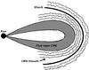 |
Fig. 1 A schematic of the CME-shock system. The CME is modeled as a flux rope structure. The undulating lines ahead of the shock denote MHD turbulence driven by the shock, while those in the CME sheath region denote turbulence in that region. |
Instead of treating the entire system shown in Fig. 1, which would be rather involved, we consider two separate models. The first, which we call the CME-only model, is one where the FD is assumed to be exclusively due to the CME, which is progressively populated by high energy cosmic rays as it propagates from the Sun to the Earth. The preliminary idea behind this model was first sketched by Cane et al. (1995) and was further developed in S09. However, the work we describe here addresses the multi-rigidity data, which is a major improvement over S09. We will describe several other salient improvements in the CME-only model in subsequent sections. The second model, which we call the shock-only model, is one where the FD is assumed to arise only as a result of a propagating diffusive barrier, which is the shock driven by the CME (e.g., Wibberenz et al. 1998). The diffusive barrier would act as a shield for the Galactic cosmic ray flux, resulting in a lower cosmic ray density behind it. In treating these two models separately we aim to identify which is the dominant contributor to the observed FD, the CME, or the shock.
We identify FDs in the GRAPES-3 data that are associated with near-Earth magnetic clouds and possibly with the shocks driven by them. We describe our criteria for shortlisting events in the next section. We then test the extent to which each of the two models satisfies the multi-rigidity FD data from the GRAPES-3 muon telescope. In the subsequent analysis the use of cutoff rigidity rather than median rigidity is preferred for the following reason. The cutoff rigidity in a given direction represents the threshold rigidity of incoming cosmic rays and the magnitude of FD is a sensitive function of it. Instead, the median rigidity is comparatively insensitive to the magnitude of the FD.
2. Criteria for shortlisting events
Selected events.
2.1. First and second shortlists: characteristics of the FD
We have examined all FD events observed by the GRAPES-3 muon telescope from 2001 to 2004. We then shortlisted events that have magnitudes >0.25% and possess a relatively clean profile comprising a sudden decrease followed by a gradual exponential recovery. While the figure of 0.25% might seem rather small by neutron monitor standards, we emphasize that the largest events observed with GRAPES-3 have magnitudes of ~1%. This list, which contains 72 events, is called shortlist 1. We next correlate the events in shortlist 1 with lists of magnetic clouds near the Earth observed by the WIND and ACE spacecrafts (Huttunen et al. 2005; Lynch et al. 2003; A. Lara, priv. comm.) and select only those that can be connected reasonably well with a near-Earth magnetic cloud, and this set is labeled shortlist 2 (Table 1). The decrease minimum for most of the FD events in shortlist 2 lie between the start and the end of the near-Earth magnetic cloud.
2.2. Third shortlist: CME velocity profile
Since we are looking for FD events that are associated with shocks as well as CMEs, we examine the CME catalog1 for a near-Sun CME that can reasonably correspond to the near-Earth magnetic cloud that we associated with the FD in forming shortlist 2. In S09 it was assumed that the CME propagates with a constant speed from the Sun to the Earth. In this paper, we adopt a more realistic, two-step velocity profile described below.
The data from the LASCO coronograph aboard the SOHO spacecraft11 provide details about CME propagation up to a distance of ≈30
R⊙ from the Sun. We fit the velocity profile to the LASCO
data points  (1)where
vi and ai are the initial
velocity and acceleration of CME, respectively, and Rm is the
heliocentric distance at which the CME is last observed in the LASCO field of view. For
distances >Rm, we assume that the CME dynamics are
governed exclusively by the aerodynamic drag it experiences due to momentum coupling with
the ambient solar wind. For heliocentric distances >Rm,
we therefore use the widely used one-dimensional differential equation to determine the
CME velocity profile: (e.g., Borgazzi et al. 2009)
(1)where
vi and ai are the initial
velocity and acceleration of CME, respectively, and Rm is the
heliocentric distance at which the CME is last observed in the LASCO field of view. For
distances >Rm, we assume that the CME dynamics are
governed exclusively by the aerodynamic drag it experiences due to momentum coupling with
the ambient solar wind. For heliocentric distances >Rm,
we therefore use the widely used one-dimensional differential equation to determine the
CME velocity profile: (e.g., Borgazzi et al. 2009)
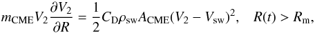 (2)where
mCME is the CME mass, CD is the
dimensionless drag coefficient, ρsw is the solar wind density,
(2)where
mCME is the CME mass, CD is the
dimensionless drag coefficient, ρsw is the solar wind density,
 is the cross-sectional area of the CME, and Vsw is the solar
wind speed. The boundary condition used is
V2 = vm at
R(t) = Rm. The CME mass
mCME is assumed to be 1015 g and the solar wind
speed Vsw is taken to be equal to 450 km s-1. The
solar wind density ρsw is given by the model of Leblanc et al.
(1998). The composite velocity profile for the
CME is defined by
is the cross-sectional area of the CME, and Vsw is the solar
wind speed. The boundary condition used is
V2 = vm at
R(t) = Rm. The CME mass
mCME is assumed to be 1015 g and the solar wind
speed Vsw is taken to be equal to 450 km s-1. The
solar wind density ρsw is given by the model of Leblanc et al.
(1998). The composite velocity profile for the
CME is defined by 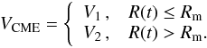 (3)The
total travel time for the CME is
(3)The
total travel time for the CME is  , where
Ri is the heliocentric radius at which the CME is first
detected and Rf is equal to 1 AU. We have used a constant drag
coefficient CD and adjusted its value so that the total travel
time thus calculated matches the time elapsed between the first detection of the CME in
the LASCO FOV and its detection as a magnetic cloud near the Earth. We have retained only
those events for which it is possible to find a constant CD
and this criterion is satisfied. We have also eliminated magnetic clouds that could be
associated with multiple CMEs. This defines our final shortlist, which we call shortlist
3. The events that have an entry in the last column labeled CME launch in Table 1 comprise shortlist 3. We note that we have adjusted
the parameter CD so that the final CME speed obtained from Eq.
(2) is close to the observed magnetic
cloud speed near the Earth. It is usually not possible to find a
CD that will yield an exact match for the velocities and for
the total travel times (e.g., Lara et al. 2011).
Figure 2 shows an example of the composite velocity
profile (given by Eqs. (1) and (2)) for a representative CME that was first
observed in the LASCO FOV on 2001 November 22, and that resulted in a FD on 2001 November
24.
, where
Ri is the heliocentric radius at which the CME is first
detected and Rf is equal to 1 AU. We have used a constant drag
coefficient CD and adjusted its value so that the total travel
time thus calculated matches the time elapsed between the first detection of the CME in
the LASCO FOV and its detection as a magnetic cloud near the Earth. We have retained only
those events for which it is possible to find a constant CD
and this criterion is satisfied. We have also eliminated magnetic clouds that could be
associated with multiple CMEs. This defines our final shortlist, which we call shortlist
3. The events that have an entry in the last column labeled CME launch in Table 1 comprise shortlist 3. We note that we have adjusted
the parameter CD so that the final CME speed obtained from Eq.
(2) is close to the observed magnetic
cloud speed near the Earth. It is usually not possible to find a
CD that will yield an exact match for the velocities and for
the total travel times (e.g., Lara et al. 2011).
Figure 2 shows an example of the composite velocity
profile (given by Eqs. (1) and (2)) for a representative CME that was first
observed in the LASCO FOV on 2001 November 22, and that resulted in a FD on 2001 November
24.
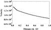 |
Fig. 2 Velocity profile for the CME corresponding to the 2001 November 24 FD event. The CME was first observed in the LASCO FOV on 2001 November 22. The solid line shows the first stage governed by LASCO observations Eq. (1), where the CME is assumed to have a constant deceleration. The dashed line shows the second stage Eq. (2), where the CME is assumed to experience an aerodynamic drag characterized by a constant CD. |
3. Models for FDs
We apply two different models to the FD events in Table 1; the first one is the CME-only model, which assumes that the FD owes its origin only to the CME. The second one is the shock-only model, which assumes that the FD is exclusively due to the shock, which is approximated as a diffusive barrier. Although both the shock and the CME are expected to contribute to the FD, our treatment seeks to determine which one of them is the dominant contributor at rigidities ranging from 14 to 24 GV. Before describing the models, we discuss the perpendicular diffusion coefficient.
3.1. Perpendicular diffusion coefficient
We use an isotropic perpendicular diffusion coefficient (D⊥) to characterize the penetration of cosmic rays across large scale, ordered magnetic fields. We envisage a CME, which has a flux rope structure, propagates outwards from the Sun, driving a shock ahead of it (see, e.g., Vourlidas et al. 2012). The flux rope CME-shock geometry is illustrated in Fig. 1. The CME sheath region between the CME and the shock is known to be turbulent (e.g., Manoharan et al. 2000) and it is well accepted that it has a significant role to play in determining FDs (Badruddin 2002; Yu et al. 2010). The isotropic perpendicular diffusion coefficient D⊥ characterizes the penetration of cosmic rays through the ordered, compressed large-scale magnetic field near the shock, and across the ordered magnetic field of the flux rope CME. In diffusing across the shock, the cosmic rays are affected by the turbulence ahead of the shock, and in diffusing across the magnetic fields bounding the flux rope CME, the cosmic rays are affected by the turbulence in the CME sheath region.
The subject of charged particle diffusion across field lines in the presence of turbulence is a subject of considerable research. Analytical treatments include the so-called classical scattering theory (e.g., Giacalone & Jokipii 1999, and references therein), and the nonlinear guiding center theory (Matthaeus et al. 2003; Shalchi 2010) for perpendicular diffusion. Numerical treatments include Giacalone & Jokipii (1999), Casse et al. (2002), Candia & Roulet (2004) and Tautz & Shalchi (2011). For our purposes, we seek a concrete, usable prescription for the D⊥ that can incorporate as many observationally determined quantities as possible. We find that the analytical fits to extensive numerical simulations provided by Candia & Roulet (2004), best suit our requirements. We note, in particular, that their results not only reproduce the standard results of Giacalone & Jokipii (1999) and Casse et al. (2002) but also extend the regime of validity to include strong turbulence and high rigidities. Our approach is similar to that of Effenberger et al. (2012), who adopt empirical expressions for the perpendicular diffusion coefficients. It should be mentioned, however, that they allow for the possibility of anisotropic perpendicular diffusion. We treat the case of radial diffusion across the largely azimuthal magnetic fields bounding a flux rope CME structure, and we therefore need only one (isotropic) perpendicular diffusion coefficient (D⊥).
In the formulation of Candia & Roulet (2004), the perpendicular diffusion coefficient D⊥ is a
function of the quantity ρ (which is closely related to the rigidity and
indicates how tightly the proton is bound to the magnetic field) and the level of
turbulence σ2. Our characterization of
D⊥(ρ,σ2)
follows that of S09, who adopt the analytical fits to Monte Carlo simulations of particle
transport in turbulent magnetic fields given by Candia & Roulet (2004). The quantity ρ is related to the
rigidity Rg by  (4)where
RL is the Larmor radius and B0
is the strength of the relevant large-scale magnetic field. For the CME-only model,
B0 refers to the large-scale magnetic field bounding the
CME, and for the shock-only model, it refers to the enhanced large-scale magnetic field at
the shock. In writing second step in Eq. (4), we have related the Larmor radius to the rigidity
Rg by
(4)where
RL is the Larmor radius and B0
is the strength of the relevant large-scale magnetic field. For the CME-only model,
B0 refers to the large-scale magnetic field bounding the
CME, and for the shock-only model, it refers to the enhanced large-scale magnetic field at
the shock. In writing second step in Eq. (4), we have related the Larmor radius to the rigidity
Rg by  (5)For the CME-only
model, we adopt
Lmax = 2 R(T), where
R(T) is the radius of the near-Earth magnetic cloud.
This is in contrast with S09, where Lmax was taken to be
106 km, which is the approximate value for the outer scale of the turbulent
cascade in the solar wind. For the shock-only model, on the other hand, we assume that
Lmax is equal to 1 AU.
(5)For the CME-only
model, we adopt
Lmax = 2 R(T), where
R(T) is the radius of the near-Earth magnetic cloud.
This is in contrast with S09, where Lmax was taken to be
106 km, which is the approximate value for the outer scale of the turbulent
cascade in the solar wind. For the shock-only model, on the other hand, we assume that
Lmax is equal to 1 AU.
The turbulence level σ2 is defined (as in Candia &
Roulet 2004, and S09) to be  (6)where
Br is the fluctuating part of the turbulent magnetic field
and the angular braces denote an ensemble average.
(6)where
Br is the fluctuating part of the turbulent magnetic field
and the angular braces denote an ensemble average.
For the sake of completeness, we reproduce the full expression for the isotropic
perpendicular diffusion coefficient that we use in this work. It is the same as the one
used in S09, and is taken from Candia & Roulet (2004). The diffusion coefficient due to scattering of particles along the mean
magnetic field D∥ is given by 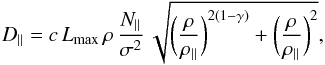 (7)where c
is the speed of light and the quantities N∥,
γ and ρ∥ are constants specific for
different kinds of turbulence. The perpendicular diffusion coefficient
(D⊥) is related to the parallel coefficient
(D∥) by
(7)where c
is the speed of light and the quantities N∥,
γ and ρ∥ are constants specific for
different kinds of turbulence. The perpendicular diffusion coefficient
(D⊥) is related to the parallel coefficient
(D∥) by 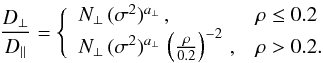 (8)The
quantities N⊥ and a⊥ are constants
specific to different kinds of turbulent spectra. In this work, we assume the Kolmogorov
turbulence spectrum in our calculations. We use N∥ = 1.7,
γ = 5/3, ρ∥ = 0.20,
N⊥ = 0.025, and a⊥ = 1.36 (Table
1, Candia & Roulet 2004). Equation (7) together with Eq. (8) defines the isotropic perpendicular
diffusion coefficient we use in this work.
(8)The
quantities N⊥ and a⊥ are constants
specific to different kinds of turbulent spectra. In this work, we assume the Kolmogorov
turbulence spectrum in our calculations. We use N∥ = 1.7,
γ = 5/3, ρ∥ = 0.20,
N⊥ = 0.025, and a⊥ = 1.36 (Table
1, Candia & Roulet 2004). Equation (7) together with Eq. (8) defines the isotropic perpendicular
diffusion coefficient we use in this work.
3.2. CME-only model
The basic features of the CME-only model are similar to the one used in S09 and here we only highlight the areas where there are significant differences from S09. There are practically no high-energy Galactic cosmic rays inside the CME when it starts out near the Sun. The cosmic rays diffuse into it from the surroundings via perpendicular diffusion across the closed magnetic field lines as it propagates through the heliosphere as shown schematically in Fig. 3. Near the Earth, the difference between the (relatively lower) cosmic ray proton density inside the CME and that in the ambient medium appears as the FD. We then obtain an estimate of the cosmic ray proton density inside the CME produced by the cumulative effect of diffusion.
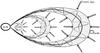 |
Fig. 3 An illustration depicting a flux rope CME expanding and propagating away from the Sun. High-energy Galactic cosmic rays diffuse into the CME across its bounding magnetic field. |
The flux F of protons diffusing into the CME at a given time depends on
the isotropic perpendicular diffusion coefficient D⊥ and the
density gradient
∂Na/∂r,
and can be written as 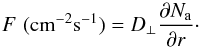 (9)As mentioned
earlier, the D⊥ characterizes diffusion across the (largely
closed) magnetic fields bounding the CME, and Na is the
ambient density of high energy protons. The total number of cosmic ray protons that will
have diffused into the CME after a time T is related to the diffusing
flux by
(9)As mentioned
earlier, the D⊥ characterizes diffusion across the (largely
closed) magnetic fields bounding the CME, and Na is the
ambient density of high energy protons. The total number of cosmic ray protons that will
have diffused into the CME after a time T is related to the diffusing
flux by 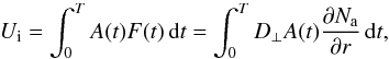 (10)where A(t) is the
cross-sectional area of the CME at a given time t. According to our
convention, the CME is first observed in the LASCO FOV at t = 0 and
reaches the Earth at t = T. The ambient density gradient
∂Na/∂r
is approximated by the expression
(10)where A(t) is the
cross-sectional area of the CME at a given time t. According to our
convention, the CME is first observed in the LASCO FOV at t = 0 and
reaches the Earth at t = T. The ambient density gradient
∂Na/∂r
is approximated by the expression  (11)which is
significantly different from that used in S09, where L is the gradient
lengthscale. Observations of the density gradient lengthscale L exist
only for a few rigidities. We use the observations of Heber et al. (2008), who quote a value of L-1 = 4.7%
AU-1 for 1.2 GV protons. We take this as our reference value. In order to
calculate L for other rigidities (in the 14−24 GV range that we use
here), we assume that
(11)which is
significantly different from that used in S09, where L is the gradient
lengthscale. Observations of the density gradient lengthscale L exist
only for a few rigidities. We use the observations of Heber et al. (2008), who quote a value of L-1 = 4.7%
AU-1 for 1.2 GV protons. We take this as our reference value. In order to
calculate L for other rigidities (in the 14−24 GV range that we use
here), we assume that  . This
is broadly consistent with the observation (De Simone et al. 2011) that the density gradient lengthscale is only weakly dependent on
rigidity. For a given rigidity, we also need the value of L all the way
from the Sun to the Earth. In order to calculate this, we recognize that
L near the CME/magnetic cloud will not be the same as its value in the
ambient solar wind. We adopt
L ∝ Ba/BMC,
where BMC is the large-scale magnetic field bounding the CME
and Ba is the (weaker) magnetic field in the ambient medium
outside the CME. Furthermore, while BMC varies according to
Eq. (12) below, the ambient field
Ba of the Parker spiral in the ecliptic plane varies
inversely with heliocentric distance.
. This
is broadly consistent with the observation (De Simone et al. 2011) that the density gradient lengthscale is only weakly dependent on
rigidity. For a given rigidity, we also need the value of L all the way
from the Sun to the Earth. In order to calculate this, we recognize that
L near the CME/magnetic cloud will not be the same as its value in the
ambient solar wind. We adopt
L ∝ Ba/BMC,
where BMC is the large-scale magnetic field bounding the CME
and Ba is the (weaker) magnetic field in the ambient medium
outside the CME. Furthermore, while BMC varies according to
Eq. (12) below, the ambient field
Ba of the Parker spiral in the ecliptic plane varies
inversely with heliocentric distance.
We assume that the magnetic flux associated with the CME is frozen-in with it as it
propagates. In other words, the product of the CME magnetic field and the CME
cross-sectional area remains constant. This is a fairly well-founded assumption (e.g.,
Kumar & Rust 1996; Subramanian & Vourlidas 2007). One can therefore relate the CME magnetic field
B0(t) at a given time t to
the value BMC measured in the near-Earth magnetic cloud by
![Mathematical equation: \begin{equation} B_0(t) = B_{\rm MC} {\left[ \frac{R(T)}{R(t)} \right]}^2\, , \label{BFL} \end{equation}](/articles/aa/full_html/2013/07/aa20830-12/aa20830-12-eq83.png) (12)where
R(T) is the radius of the magnetic cloud observed from
the Earth and R(t) is its radius at any other time
t during its passage from the Sun to the Earth. The CME radius
R(t) and R(T) are
related via Eq. (15) below. We emphasize
that the magnetic field in Eq. (12) refers
to the magnetic field bounding the CME, and not the ambient magnetic field outside it.
(12)where
R(T) is the radius of the magnetic cloud observed from
the Earth and R(t) is its radius at any other time
t during its passage from the Sun to the Earth. The CME radius
R(t) and R(T) are
related via Eq. (15) below. We emphasize
that the magnetic field in Eq. (12) refers
to the magnetic field bounding the CME, and not the ambient magnetic field outside it.
We model the CME as an expanding cylindrical flux rope whose length increases with time
as it propagates outwards. Its cross-sectional area at time t is
 (13)where
L(t) is the length of the flux-rope cylinder at time
t, and is related to the height H(t)
of the CME above the solar limb via
(13)where
L(t) is the length of the flux-rope cylinder at time
t, and is related to the height H(t)
of the CME above the solar limb via  (14)We note that Eq.
(14) differs from the definition used in
S09 by a factor of 2. We assume that the CMEs expand in a self-similar manner as they
propagate outwards. The three dimensional flux rope fittings to CMEs in the ~2−20
R⊙ field of view using SECCHI/STEREO data validate this
assumption (e.g., Poomvises et al. 2010). The
self-similar assumption means that the radius of the
R(t) of the flux rope is related to its heliocentric
height H(t) by
(14)We note that Eq.
(14) differs from the definition used in
S09 by a factor of 2. We assume that the CMEs expand in a self-similar manner as they
propagate outwards. The three dimensional flux rope fittings to CMEs in the ~2−20
R⊙ field of view using SECCHI/STEREO data validate this
assumption (e.g., Poomvises et al. 2010). The
self-similar assumption means that the radius of the
R(t) of the flux rope is related to its heliocentric
height H(t) by  (15)where
H(T), the heliocentric height at time
T, is =1 AU by definition, and R(T)
is the measured radius of the magnetic cloud from the Earth.
(15)where
H(T), the heliocentric height at time
T, is =1 AU by definition, and R(T)
is the measured radius of the magnetic cloud from the Earth.
As mentioned earlier, we consider a two-stage velocity profile for CME propagation, expressed by Eqs. (1) and (2); this is substantially different from the constant speed profile adopted in S09.
Using Eqs. (11), (13) and (14) in (10), we get
the expression for the total number of protons inside the CME when it arrives on the Earth
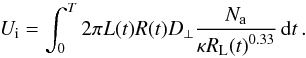 (16)The cosmic ray
density inside the CME when it arrives on the Earth is
(16)The cosmic ray
density inside the CME when it arrives on the Earth is  (17)where
L(T) and R(T) are
the length and cross-sectional radius of the CME, respectively, at time
T, when it reaches the Earth. When the CME arrives on the Earth, the
relative difference between the cosmic ray density inside the CME and the ambient
environment is manifested as the FD, whose magnitude M can be written as
(17)where
L(T) and R(T) are
the length and cross-sectional radius of the CME, respectively, at time
T, when it reaches the Earth. When the CME arrives on the Earth, the
relative difference between the cosmic ray density inside the CME and the ambient
environment is manifested as the FD, whose magnitude M can be written as
 (18)We compare the
value of the FD magnitude M predicted by Eq. (18) with observations in Sect. 4.
(18)We compare the
value of the FD magnitude M predicted by Eq. (18) with observations in Sect. 4.
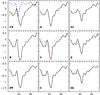 |
Fig. 4 Muon flux along the nine directions is shown for the FD on 2001 November 24. The fluxes are shown as percentage deviations from mean values. The solid black lines show the data after applying a low-pass filter (S09). The blue dashed line in the first panel shows the magnetic field observed in-situ by spacecraft. The magnetic field data are inverted (i.e., magnetic field peaks appear as troughs) and are scaled to fit in the panel. The red dotted line in the middle panel shows Tibet neutron monitor data scaled down by a factor of 3 to fit in the panel. |
An example of an FD event observed in all 9 bins of GRAPES-3 is shown in Fig. 4. The x-axis is the time in days starting from 2001 November 1 and the y-axis gives the percentage deviation of the muon flux from the pre-event mean. The magnitude M of the FD for a given rigidity bin is the difference between the pre-event cosmic ray intensity and the intensity at the minimum of the FD.
3.3. Shock-only model
In this approach, we assume that the FD is caused exclusively by the shock, which is
modeled as a propagating diffusive barrier. The expression for the magnitude of the FD
according to this model is (Wibberenz et al. 1998)
 (19)where
Ua is the ambient cosmic ray density and
Ushock is that inside the shock,
D⊥a is the ambient isotropic perpendicular
diffusion coefficient and D⊥shock is that inside
the shock, Vsw is the solar wind velocity, and
Lshock is the shock sheath thickness. For each shock event,
we examine the magnetic field data from the ACE and WIND spacecrafts and estimate the
shock sheath thickness Lshock to be the spatial extent of the
magnetic field enhancement. An example is shown in Fig. 5.
(19)where
Ua is the ambient cosmic ray density and
Ushock is that inside the shock,
D⊥a is the ambient isotropic perpendicular
diffusion coefficient and D⊥shock is that inside
the shock, Vsw is the solar wind velocity, and
Lshock is the shock sheath thickness. For each shock event,
we examine the magnetic field data from the ACE and WIND spacecrafts and estimate the
shock sheath thickness Lshock to be the spatial extent of the
magnetic field enhancement. An example is shown in Fig. 5.
In computing D⊥a and
D⊥shock we need to use different values for the
proton rigidity ρ for the ambient medium and in the shock sheath; they
are related to the proton rigidity Rg by  where
where
 is the
ambient magnetic field and
is the
ambient magnetic field and  is the
magnetic field inside the shock sheath.
is the
magnetic field inside the shock sheath.
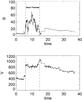 |
Fig. 5 Interplanetary magnetic field and solar wind speed from the day 2001 November 24, The shock sheath thickness is computed by multiplying the time interval inside the dotted lines by the solar wind speed. |
4. Results
In this section we first describe various parameters needed for the CME-only and the shock-only models that are derived from observations. Using these parameters, we examine whether the notion of cosmic ray diffusion is valid for each model. Using the observationally determined parameters, we can determine which of the two models best reproduces the observed FD magnitude in each rigidity bin.
4.1. Observationally derived parameters
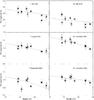 |
Fig. 6 FD magnitude observed with GRAPES-3 (∗ symbols). The dashed line is obtained using the CME-only model. |
Table A.2 contains the observationally determined parameters for each of the CMEs and their corresponding shocks in the final shortlist (Table 1).
The quantity First obs denotes the time (in UT) when the CME was first observed in the
LASCO FOV, while Rfirst is the distance (in units of
R⊙) at which CME was first observed in LASCO FOV and
Rlast is the distance at which the CME was last observed in
LASCO FOV. The quantity Vexp is the speed of CME at
Rlast (in km s-1) and
ai is the acceleration of CME in the LASCO FOV (in
m s-2). The quantity CD is the (constant)
dimensionless drag coefficient used for the velocity profile (Sect. 2.2). The quantities MC start and MC end denote the start and end times
of the magnetic cloud in UT. The quantity  is solar
wind speed at the Earth (in km s-1) just ahead of the arrival of the magnetic
cloud, and RMC is the radius of the magnetic cloud (in km).
The quantity BMC is the peak magnetic field inside the
magnetic cloud (in nT). The quantity Ttotal is the Sun-Earth
travel time (in h) taken by the CME to travel from Sun to Earth. The quantity Shock
arrival denotes the time (in UT) when the shock is detected near the Earth. The quantities
Ba and Bshock represent the
magnetic fields (in nT) in the ambient solar wind and inside the shock sheath region,
respectively (see Fig. 5 for an example). The
quantity
is solar
wind speed at the Earth (in km s-1) just ahead of the arrival of the magnetic
cloud, and RMC is the radius of the magnetic cloud (in km).
The quantity BMC is the peak magnetic field inside the
magnetic cloud (in nT). The quantity Ttotal is the Sun-Earth
travel time (in h) taken by the CME to travel from Sun to Earth. The quantity Shock
arrival denotes the time (in UT) when the shock is detected near the Earth. The quantities
Ba and Bshock represent the
magnetic fields (in nT) in the ambient solar wind and inside the shock sheath region,
respectively (see Fig. 5 for an example). The
quantity  represents the near-Earth shock speed in km s-1.
Table A.1 contains details of the FDs associated with each of the CMEs in the final shortlist. The magnitude of the FD in a given rigidity bin is the difference between the pre-event intensity of the cosmic rays and the intensity at the minimum of the FD. It also contains the onset and the time of minimum, and the magnitude of the decrease in each bin (together with the corresponding cutoff rigidity) for each of the FD events in our final shortlist.
4.2. Fitting the CME-only and shock-only models to multi-rigidity FD data
Using the observational parameters listed in Table A.2, we have computed the magnitude of the FD using the CME-only (Sect. 3.2) and shock-only models (Sect. 3.3). The only free parameter in our model is the ratio of the energy
density in the random magnetic fields to that in the large scale magnetic field
σ2 ≡ ⟨ Bturb2/B02 ⟩.
Figure 6 shows the best fits of the CME-only model to
the multi-rigidity data. The only free parameter in the model is
σ2 ≡ ⟨ Bturb2/B02 ⟩
, and the best fit is chosen by minimizing the χ2 with respect
to σ2. For each FD event, the ∗ symbols denote the observed FD
magnitude for a given rigidity bin. The dashed line denotes the FD magnitude predicted by
the CME-only model. We define the chi-square statistic as 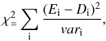 (22)where
Ei is the value predicted by the theoretical model,
Di is the corresponding GRAPES-3 data point, and
vari is the variance for the corresponding data points. The
χ2 values obtained after minimizing with respect to
σ2 are listed in Table 2.
(22)where
Ei is the value predicted by the theoretical model,
Di is the corresponding GRAPES-3 data point, and
vari is the variance for the corresponding data points. The
χ2 values obtained after minimizing with respect to
σ2 are listed in Table 2.
Minimum χ2 values for the CME-only model fits to GRAPES-3 data.
Turbulence levels in the sheath region required by the models.
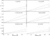 |
Fig. 7 f0 ≡ RL/R versus distance as a CME propagates from the Sun to the Earth. The dashed and continuous lines represent 24 GV and 12 GV protons, respectively. |
The entries in the second column σMC in Table 3 denote the square roots of the turbulence parameter σ2 that we have used for the model fits for each event. These values represent the level of turbulence in the sheath region immediately ahead of the CME, through which the cosmic rays must traverse in order to diffuse into the CME. By comparison, the value of σ for the quiescent solar wind ranges from 6 to 15% (Spangler 2002). Evidently, the CME-only model implies that the sheath region ahead of the CME is only a little more turbulent than the quiescent solar wind, except for the 2004 July 26 event, where the speed of CME at the Earth was much higher than that for the other events.
We have carried out a similar exercise for the shock-only model (Sect. 3.3). For each event, we have used the observationally obtained parameters pertaining to the shock listed in Table A.2. Since this model needs the turbulence levels in both the ambient medium and the shock sheath region to be specified, we have assumed that the turbulence level inside the shock sheath region is twice that in the ambient medium. We find that it is not possible to fit the shock-only model to the multi-rigidity data using values for the turbulence parameter that are reasonably close to that in the quiescent solar wind. For each event, the column labeled σShock in Table 3 denotes the turbulence level in the shock sheath region that is required to obtain a reasonable fit to the data. Clearly, these values are an order of magnitude higher than those observed in the quiet solar wind.
4.3. RL/RCME for CME-only model
Kubo & Shimazu (2010) have simulated the process of cosmic ray diffusion into an ideal flux rope CME in the presence of MHD turbulence. They find that, if the quantity f0(t) ≡ RL(t)/R(t) is small, cosmic ray penetration into the flux rope is dominated by diffusion via turbulent irregularities. Other effects such as gradient drift due to the curvature of the magnetic field are unimportant under these conditions. Figure 7 shows the quantity f0(t) ≡ RL(t)/R(t) for 12 and 24 GV protons, for each of the CMEs in our final shortlist (Table 1). The Larmor radius RL(t) is defined by Eqs. (5) and (12) and the CME radius R(t) is defined in Eq. (15). Clearly, f0 ≪ 1 all through the Sun-Earth passage of the CMEs, and this means that the role of MHD turbulence in aiding penetration of cosmic rays into the flux rope structure is expected to be important.
5. Summary
Our main aim in this work is to determine whether FDs due to cosmic rays of rigidities ranging from 14 to 24 GV are caused primarily by the CME, or by the shock associated with it. We examine this question in the context of multi-rigidity FD data from the GRAPES-3 instrument. We use a carefully selected sample of FD events from GRAPES-3 that are associated with both CMEs and shocks.
We consider two models: the CME-only model (Sect. 3.2) and the shock-only model (Sect. 3.3). In the CME-only model, we envisage the CME as an expanding bubble bounded by large-scale magnetic fields. The CME starts out near the Sun with practically no high energy cosmic rays inside it. As it travel towards the Earth, high-energy cosmic rays diffuse into the CME across the large-scale magnetic fields bounding it. The diffusion coefficient is a function of the rigidity of the cosmic ray particles as well as the level of MHD turbulence in the vicinity of the CME (the sheath region). Despite the progressive diffusion of cosmic rays into it, the cosmic ray density inside the CME is still lower than the ambient density when it reaches the Earth. When the CME engulfs the Earth, this density difference causes the FD observed by cosmic ray detectors. In the shock-only model, we consider the shock as a propagating diffusive barrier. It acts as an umbrella against cosmic rays, and the cosmic ray density behind the umbrella is lower than that ahead of it.
We have obtained a list of FD events observed by the GRAPES-3 instrument using the shortlisting criteria described in Sect. 2. For each of these shortlisted events, we have used observationally derived parameters listed in Table A.2 for both the models. The only free parameter was the level of MHD turbulence (defined as the square root of the energy density in the turbulent magnetic fluctuations to that in the large-scale magnetic field) in the sheath region.
6. Conclusions
Figure 6 shows the results of the CME-only model fits to multi-rigidity data for each of the shortlisted events. For the shock-only model, we use the turbulence level in the shock sheath region as the free parameter. Table 3 summarizes the values of these turbulence levels that we have used for each of the FD events in the final shortlist. These values may be compared with the estimate of 6 to 15% for the turbulence level in the quiescent solar wind (Spangler 2002). We thus find that a good model fit using the CME-only model requires a turbulence level in the sheath region that is typically only a little higher than that in the quiescent solar wind, which is generally consistent with observations. On the other hand, a good fit using the shock-only model demands a turbulence level in the shock sheath region that is often an order of magnitude higher than that in the quiet solar wind, which is somewhat unrealistic. The results summarized in Table 3, imply that, for FDs involving protons of rigidities ranging from 14 to 24 GV, the CME-only model is a viable one, while the shock-only model is not. Given the remarkably good fits to multi-rigidity data (Fig. 6), the reasonable turbulence levels in the sheath region demanded by the CME-only model (Table 3) and because the FD minima usually occur well within the magnetic cloud (Table A.1), we conclude that CMEs are the dominant contributors to the FDs observed by the GRAPES-3 experiment.
Online material
Appendix A: Tables
Derived parameters of FD for events.
Observed parameters of CME & Shock for different events.
Acknowledgments
K.P. Arunbabu acknowledges support from a Ph.D. studentship at IISER Pune. P. Subramanian acknowledges partial support from the RESPOND program administered by the Indian Space Research Organization. We thank Alejandro Lara for useful discussions and the referee K. Scherer for several critical and helpful suggestions. We thank D. B. Arjunan, A. Jain, the late S. Karthikeyan, K. Manjunath, S. Murugapandian, S. D. Morris, B. Rajesh, B. S. Rao, C. Ravindran, and R. Sureshkumar for their help in the testing, installation, and operating the proportional counters and the associated electronics and during data acquisition. We thank G. P. Francis, I. M. Haroon, V. Jeyakumar, and K. Ramadass for their help in the fabrication, assembly, and installation of various mechanical components and detectors.
References
- Badruddin 2002, Ap&SS, 281, 651 [NASA ADS] [CrossRef] [Google Scholar]
- Badruddin,Yadav, R. S., & Yadav, N. R. 1986, Sol. Phys., 105, 413 [NASA ADS] [CrossRef] [Google Scholar]
- Blanco, J. J., Catalan, E., Hidalgo, M. A., Medina, J., & Rodiguez-Pacheco, J. 2013, Sol. Phys., DOI: 10.1007/s11207-013-0256-1 [Google Scholar]
- Bothmer, V., & Schwenn, R. 1998, Ann. Geophys., 16, 1 [Google Scholar]
- Borgazzi, A., Lara, A., Echer, E., et al. 2009, A&A, 498, 885 [NASA ADS] [CrossRef] [EDP Sciences] [Google Scholar]
- Burlaga, L. F., Sittler, E., Mariani, F., & Schwenn, R. 1981, J. Geophys. Res., 86, 6673 [Google Scholar]
- Candia, J., & Roulet, E. 2004, J. Cosmol. Astropart. Phys., 10, 7 [Google Scholar]
- Cane, H. V. 2000, Space Sci. Rev., 93, 55 [NASA ADS] [CrossRef] [Google Scholar]
- Cane, H. V., Richardson, I. G., & Wibberenz, G. 1995, Proc. 24th Int. Cosmic Ray Conf., 4, 377 [Google Scholar]
- Casse, F., Lemoine, M., & Pelletier, G. 2002, Phys. Rev. D, 65, 023002 [Google Scholar]
- de Simone, N., di Felice, V., Gieseler, J., et al. 2011, ASTRA, 7, 425 [Google Scholar]
- Effenberger, F., Fichtner, H., Scherer, K., et al. 2012, ApJ, 750, 108 [NASA ADS] [CrossRef] [Google Scholar]
- Giacalone, J., & Jokipii, J. R. 1999, ApJ, 520, 204 [Google Scholar]
- Hayashi, Y., Aikawa, Y., Gopalakrishnan, N. V., et al. 2005, Nucl. Instrum. Meth. A, 545, 643 [Google Scholar]
- Heber, B., Gieseler, J., Dunzlaff, P., et al. 2008, ApJ, 689, 1443 [NASA ADS] [CrossRef] [Google Scholar]
- Huttunen, K. E. J., Schwenn, R., Bothmer, V., & Koskinen, H. E. J. 2005, Ann. Geophys., 23, 625 [NASA ADS] [CrossRef] [Google Scholar]
- Kubo, Y., & Shimazu, H. 2010, ApJ, 720, 853 [NASA ADS] [CrossRef] [Google Scholar]
- Kuwabara, T., Bieber, J. W., Evensen, P., et al. 2009, J. Geophys. Res., 114, 05109 [Google Scholar]
- Lara, A., Flandes, A., Borgazzi, A., & Subramanian, P. 2011, J. Geophys. Res., 116, CiteID A12102 [Google Scholar]
- Leblanc, Y., Dulk, G. A., Bougeret, J.-L., et al. 1998, Sol. Phys., 183, 165 [NASA ADS] [CrossRef] [Google Scholar]
- Lockwood, J. A., Webber, W. R., & Debrunner, H. 1991, J. Geophys. Res., 96, 11587 [NASA ADS] [CrossRef] [Google Scholar]
- Lynch, B. J., Zurbuchen, T. H., Fisk, L. A., & Antiochos, S. K. 2003, J. Geophys. Res., 108, 1239 [Google Scholar]
- Manoharan, P. K., Kojima, M., Gopalswamy, N., et al. 2000, ApJ, 530, 1061 [NASA ADS] [CrossRef] [Google Scholar]
- Matthaeus, W. S., Qin, G., Bieber, J. W., & Zank, G. P. 2003, ApJ, 590, L53 [Google Scholar]
- Nonaka, T., Hayashi, Y., Ito, N., et al. 2006, Phys. Rev. D, 74, 052003 [NASA ADS] [CrossRef] [Google Scholar]
- Oh, S. Y., & Yi, Y. 2012, Sol. Phys., 280, 197 [NASA ADS] [CrossRef] [Google Scholar]
- Poomvises, W.,Zhang, J.,Olmedo, O., 2010, ApJ, 717, L159 [Google Scholar]
- Reames, D. V., Kahler, S. W., & Tylka, A. J. 2009, ApJ, 700, 196 [NASA ADS] [CrossRef] [Google Scholar]
- Richardson, I. G., &Cane, H. V. 2011, Sol. Phys., 270, 609 [NASA ADS] [CrossRef] [Google Scholar]
- Sanderson, T. R., Beeck, J., Marsden, G. R., et al. 1990, Proc. 21st Int. Cosmic Ray Conf., 6, 251 [Google Scholar]
- Shalchi, A. 2010, ApJ, 720, L127 [Google Scholar]
- Schwenn, R., Dal Lago, A., Huttunen, E., & Gonzalez, W. D. 2005, Ann. Geophys., 23, 1033 [NASA ADS] [CrossRef] [Google Scholar]
- Spangler, S. R. 2002, ApJ, 576, 997 [NASA ADS] [CrossRef] [Google Scholar]
- Subramanian, P., & Vourlidas, A. 2007, A&A, 467, 685 [NASA ADS] [CrossRef] [EDP Sciences] [Google Scholar]
- Subramanian, P., Antia, H. M., Dugad, S. R., et al. 2009, A&A, 494, 1107 [Google Scholar]
- Tautz, R. C., & Shalchi, A. 2011, ApJ, 735, 92 [NASA ADS] [CrossRef] [Google Scholar]
- Vourlidas, A., Lynch, B. J., Howard, R. A., & Li, Y. 2012, Sol. Phys., 192V: DOI: 10.1007/s11207-012-0084-8 [Google Scholar]
- Wang, Y., Zhou, G., Ye, P., Wang, S., & Wang, J. 2006, ApJ, 651, 1245 [NASA ADS] [CrossRef] [Google Scholar]
- Wibberenz, G., le Roux, J. A., Potgieter, M. S., & Bieber, J. W. 1998, Space Sci. Rev., 83, 309 [NASA ADS] [CrossRef] [Google Scholar]
- Yu, X. X.,Lu, H.,Le, G. M., &Shi, F., 2010, Sol. Phys., 263, 223 [NASA ADS] [CrossRef] [Google Scholar]
- Zhang, G., & Burlaga, L. F. 1988, J. Geophys. Res., 93, 2511 [NASA ADS] [CrossRef] [Google Scholar]
All Tables
All Figures
|
Fig. 1 A schematic of the CME-shock system. The CME is modeled as a flux rope structure. The undulating lines ahead of the shock denote MHD turbulence driven by the shock, while those in the CME sheath region denote turbulence in that region. |
| In the text | |
|
Fig. 2 Velocity profile for the CME corresponding to the 2001 November 24 FD event. The CME was first observed in the LASCO FOV on 2001 November 22. The solid line shows the first stage governed by LASCO observations Eq. (1), where the CME is assumed to have a constant deceleration. The dashed line shows the second stage Eq. (2), where the CME is assumed to experience an aerodynamic drag characterized by a constant CD. |
| In the text | |
|
Fig. 3 An illustration depicting a flux rope CME expanding and propagating away from the Sun. High-energy Galactic cosmic rays diffuse into the CME across its bounding magnetic field. |
| In the text | |
|
Fig. 4 Muon flux along the nine directions is shown for the FD on 2001 November 24. The fluxes are shown as percentage deviations from mean values. The solid black lines show the data after applying a low-pass filter (S09). The blue dashed line in the first panel shows the magnetic field observed in-situ by spacecraft. The magnetic field data are inverted (i.e., magnetic field peaks appear as troughs) and are scaled to fit in the panel. The red dotted line in the middle panel shows Tibet neutron monitor data scaled down by a factor of 3 to fit in the panel. |
| In the text | |
|
Fig. 5 Interplanetary magnetic field and solar wind speed from the day 2001 November 24, The shock sheath thickness is computed by multiplying the time interval inside the dotted lines by the solar wind speed. |
| In the text | |
|
Fig. 6 FD magnitude observed with GRAPES-3 (∗ symbols). The dashed line is obtained using the CME-only model. |
| In the text | |
|
Fig. 7 f0 ≡ RL/R versus distance as a CME propagates from the Sun to the Earth. The dashed and continuous lines represent 24 GV and 12 GV protons, respectively. |
| In the text | |
Current usage metrics show cumulative count of Article Views (full-text article views including HTML views, PDF and ePub downloads, according to the available data) and Abstracts Views on Vision4Press platform.
Data correspond to usage on the plateform after 2015. The current usage metrics is available 48-96 hours after online publication and is updated daily on week days.
Initial download of the metrics may take a while.