| Issue |
A&A
Volume 555, July 2013
|
|
|---|---|---|
| Article Number | A69 | |
| Number of page(s) | 15 | |
| Section | Astronomical instrumentation | |
| DOI | https://doi.org/10.1051/0004-6361/201219489 | |
| Published online | 03 July 2013 | |
Extended-object reconstruction in adaptive-optics imaging: the multiresolution approach
1
Departament d’Astronomia i Meteorologia i Institut de Ciències del Cosmos
(ICC), Universitat de Barcelona (UB/IEEC),
Martí i Franqués 1,
08025
Barcelona,
Spain
e-mail: This email address is being protected from spambots. You need JavaScript enabled to view it.
; This email address is being protected from spambots. You need JavaScript enabled to view it.
2
Observatori Fabra, Reial Acadèmia de Ciències i Arts de Barcelona,
Camí de l’Observatori s/n, 08002
Barcelona,
Spain
3
Fraunhofer-Institut für Optronik, Systemtechnik und Bildauswertung, Gutleuthausstraße
1, 76275
Ettlingen,
Germany
e-mail: This email address is being protected from spambots. You need JavaScript enabled to view it.
Received: 26 April 2012
Accepted: 24 April 2013
Abstract
Aims. We propose the application of multiresolution transforms, such as wavelets and curvelets, to reconstruct images of extended objects that have been acquired with adaptive-optics (AO) systems. Such multichannel approaches normally make use of probabilistic tools to distinguish significant structures from noise and reconstruction residuals. We aim to check the prevailing assumption that image-reconstruction algorithms using static point spread functions (PSF) are not suitable for AO imaging.
Methods. We convolved two images, one of Saturn and one of galaxy M100, taken with the Hubble Space Telescope (HST) with AO PSFs from the 5-m Hale telescope at the Palomar Observatory and added shot and readout noise. Subsequently, we applied different approaches to the blurred and noisy data to recover the original object. The approaches included multiframe blind deconvolution (with the algorithm IDAC), myopic deconvolution with regularization (with MISTRAL) and wavelet- or curvelet-based static PSF deconvolution (AWMLE and ACMLE algorithms). We used the mean squared error (MSE) to compare the results.
Results. We found that multichannel deconvolution with a static PSF produces generally better results than the results obtained with the myopic/blind approaches (for the images we tested), thus showing that the ability of a method to suppress the noise and track the underlying iterative process is just as critical as the capability of the myopic/blind approaches to update the PSF. Furthermore, for these images, the curvelet transform (CT) produces better results than the wavelet transform (WT), as measured in terms of MSE.
Key words: instrumentation: adaptive optics / techniques: image processing / methods: miscellaneous
© ESO, 2013
1. Introduction
The distortions introduced into images by the acquisition process in astronomical ground-based observations are well known. Apart from the most common, such as vignetting, non-zero background or bad pixels, which must be removed prior to any other analysis, atmospheric turbulence limits the spatial resolution of an image, whereas the electronic devices used to acquire and amplify the signal introduces noise. An image is also corrupted by Poisson noise from fluctuations in the number of received photons at each pixel (Andrews & Hunt 1977). The classical equation that describes the image formation process is ![Mathematical equation: \begin{equation} image = [PSF \ast object] \Diamond noise , \label{eq1} \end{equation}](/articles/aa/full_html/2013/07/aa19489-12/aa19489-12-eq1.png) (1)where ∗ denotes the convolution operation. The symbol ◇ is a pixel-by-pixel operation that reduces to simple addition when noise is additive and independent of [PSF ∗ object] , while for Poisson noise it is an operation that returns a random deviate drawn from a Poisson distribution with mean equal to [PSF ∗ object] . It is well known that direct inversion of Eq. (1) in the Fourier domain amplifies noisy frequencies close to the cut-off frequency. Hence, in the presence of noise, such a simple method cannot be used.
(1)where ∗ denotes the convolution operation. The symbol ◇ is a pixel-by-pixel operation that reduces to simple addition when noise is additive and independent of [PSF ∗ object] , while for Poisson noise it is an operation that returns a random deviate drawn from a Poisson distribution with mean equal to [PSF ∗ object] . It is well known that direct inversion of Eq. (1) in the Fourier domain amplifies noisy frequencies close to the cut-off frequency. Hence, in the presence of noise, such a simple method cannot be used.
Several deconvolution approaches have been proposed to estimate the original signal from the seeing-limited and noise-degraded data. Since Eq. (1) is an ill-posed problem, with non-unique stable solutions, one approach is to regularize the Fourier inversion to constrain possible solutions (Tikhonov et al. 1987; Bertero & Boccacci 1998). This method generally imposes a trade-off between noise amplification and the desired resolution, which generally leads to smooth solutions. Bayesian methodology (Molina et al. 2001; Starck et al. 2002b) allows a solution compatible with the statistical nature of the signal to be sought, leading to maximum likelihood estimators (MLE; Richardson 1972; Lucy 1974) or maximum a posteriori (MAP) approaches if prior information is used, e.g., the positivity of the signal or entropy (Frieden 1978; Jaynes 1982).
All these methods can be enhanced through multichannel analysis by decomposing the signal in different planes, each of them representative of a certain scale of resolution. In such a decomposition, fine details in an image are confined to some planes, whereas coarse structures are confined to others. One of the most powerful ways to perform this decomposition is by means of the wavelet transform (WT). In particular in the astronomical context, the undecimated isotropic à trous algorithm (Holschneider et al. 1989; Shensa 1992; Starck & Murtagh 1994), also known as the starlet transform, is often used. The WT creates a multiple representation of a signal, classifying its frequencies and, simultaneously, spatially localizing them in the field of view. For the specific case of the starlet transform, this can be expressed by  (2)where s is the signal being decomposed into wavelet coefficients,
  is the wavelet plane at resolution j, and
  is the residual wavelet plane. We point out that Eq. (2) provides a prescription for direct reconstruction of the original image from all the wavelet planes and the residual plane. The advantage of WT is that it allows for different strategies to be used for different wavelet planes, e.g., by defining thresholds of statistical significance.
Given the advantages of the multiresolution analysis, the aforementioned deconvolution approaches have been adapted to work in the wavelet domain. The MLE was modified into a two-channel algorithm (Lucy 1994) where the first channel corresponds to the signal contribution and the second to the background. The wavelet transform has also been applied to maximum-entropy deconvolution methods (Núñez & Llacer 1998) to segment the image and apply different regularization parameters to each region. Starck et al. (2001) generalized the method of maximum entropy within a wavelet framework, separating the problem into two stages: noise control in the image domain and smoothness in the object domain.
While WT has been widely used in astronomical image analysis and in deconvolution, the reported use (in the same context) of multi-transforms with properties that improve on or complement WT is scarce. Such methods include, among many others: waveatoms (Demanet & Ying 2007), which aim to represent signals by textures; and curvelets (Candès et al. 2006), which introduce orientation as a classification parameter together with frequency and position. Starck et al. (2002a) used the curvelet transform (CT) for Hubble Space Telescope (HST) image restoration from noisy data. They reported enhanced contrast on the image of Saturn. Lambert et al. (2006) applied CT to choose significant coefficients from astroseismic observations while Starck et al. (2004) used CT to detect non-Gaussian signatures in observations of the cosmic microwave background. Because it is believed that CT is more suitable for representing elongated features such as lines or edges, one of the goals of this paper is to introduce CT into the Bayesian framework and show how it performs on images of extended objects.
The aforementioned methods work with static point spread functions (PSFs), i.e., they do not update the PSF of an optical system that is supplied by the operator. Nevertheless, in ground-based imaging, whether with adaptive optics (AO) or without, there are always differences between science and calibration PSFs (Esslinger & Edmunds 1998). These differences may result from changes in seeing, wind speed, slowly varying aberrations due to gravity or thermal effects and, in AO imaging, from differential response of the wavefront sensor to fluxes received from the science and calibration objects. The quality of AO images is quantified with the Strehl ratio (SR), which is the ratio of the measured peak value of a point-source image to that of the diffraction-limited PSF, often given in percent. A perfect diffraction-limited image has an SR of 100% while a seeing-degraded image on a large telescope can have an SR lower than 1%. In this paper we will use the SR to quantify the mismatch between the target and calibration PSFs. This commonly occurring mismatch has prompted optical scientists, especially those working on AO systems, to investigate blind and myopic image restoration schemes (e.g. Lane 1992; Thiébaut & Conan 1995). A blind method works without any information about the PSF, while a myopic approach relies on some initial PSF estimate that is then updated until a solution for both the object and the PSF is found.
Conan et al. (1999) compared their myopic approach to a basic, “unsupervised” Richardson-Lucy scheme and found, not surprisingly, that the myopic deconvolution is more stable. Nevertheless, to our knowledge there have not been any thorough and fully fledged efforts to compare the performance of modern, static-PSF approaches to blind/myopic methods in the context of AO imaging, and so the preference for the latter algorithms still has to be justified. Our goal is to partially fill this gap. At this stage we mention that this article is a companion paper to Baena Gallé & Gladysz (2011), where we showed that a modern, static-PSF code is capable of extracting accurate differential photometry from AO images of binary stars even when given a mismatched PSF. In the current paper we extend the analysis to more complex objects and analyze the effect of noise as well as that of the mismatched PSF. We show the importance of noise control, specifically how advanced noise suppression can set off the lack of PSF-update capability for very noisy observations. More generally, we highlight the opportunities for an exchange of ideas between the communities that prefer myopic and static-PSF approaches.
The paper is organized as follows: in Sect. 2, the algorithms AWMLE, ACMLE, MISTRAL, and IDAC are described. These algorithms represent different philosophies with regard to the deconvolution problem. AWMLE and ACMLE perform a classical static-PSF deconvolution within the wavelet or curvelet domain, MISTRAL is intended for myopic use, and IDAC can be used as a blind or a myopic algorithm. Section 3 describes the datasets we used and how we applied each of the four algorithms. A brief description of the mean squared error (MSE), together with concepts of error and residual maps that we used to compare the reconstructed objects can be found in Sect. 4. Section 5 presents the performance comparison of the four algorithms mentioned above in terms of noise and PSF mismatch. Section 6 summarizes and concludes the paper.
2. Description of the algorithms
This section is not intended to describe the algorithms in detail but rather to offer a brief overview of their characteristics and their historical uses and performances. We would also like to point out that in the text to follow we do not keep the nomenclature originally used by the respective authors. We make the following attempt at standardization: the object, or unknown, is represented with o, the image or dataset is i, and the PSF is h. Upper-case notation is used for Fourier representation. The two-dimensional pixel index is r, while f is spatial frequency. The index of a wavelet/curvelet scale is represented with j, while a single frame in a multiframe approach is indexed with i. Finally, the symbol  is used for estimates.
2.1. AWMLE
The adaptive wavelet maximum likelihood estimator (AWMLE) is a Richarson-Lucy-type algorithm (Richardson 1972; Lucy 1974) that maximizes the likelihood between the dataset and the projection of a possible solution onto the data domain, considering a combination of the Poissonian shot noise, intrinsic to the signal, and the Gaussian readout noise of the detector. This maximization is performed in the wavelet domain. The decomposition of the signal into several channels allows for various strategies to be used depending on a particular channel’s scale. This is a direct consequence of the fact that in a WT decomposition the noise, together with the finest structures of the signal, will be transferred into the high-frequency channels while coarse structures will be transferred into the low-frequency channels.
The general mathematical expression that describes AWMLE is ![Mathematical equation: \begin{equation} {\hat{o}^{(n+1)}} = K {\hat{o}^{(n)}} \left[ {h^{-}} \ast \dfrac{\sum_{j} \left( {\mathit{\omega}}_{j}^{{{o}_h^{(n)}}} + {M_{j}} \left({\mathit{\omega}}_{j}^{{i'}} - {\mathit{\omega}}_{j}^{{{o}_h^{(n)}}}\right) \right)}{ {{h^{+}} \ast {\hat{o}^{(n)}}}} \right], \label{eq10} \end{equation}](/articles/aa/full_html/2013/07/aa19489-12/aa19489-12-eq18.png) (3)where o is the object to be estimated, h + is the PSF that projects the information from the object domain to the image domain, while h − is its reverse version performing the inverse operation, i.e., the projection from the image domain to the object domain. The so-called direct projection oh is an image of the object projected onto the data domain by means of the PSF at iteration n, it appears in the numerator of Eq. (3) already decomposed in its wavelet representation. The parameter
(3)where o is the object to be estimated, h + is the PSF that projects the information from the object domain to the image domain, while h − is its reverse version performing the inverse operation, i.e., the projection from the image domain to the object domain. The so-called direct projection oh is an image of the object projected onto the data domain by means of the PSF at iteration n, it appears in the numerator of Eq. (3) already decomposed in its wavelet representation. The parameter  is a constant to conserve the energy.
The variable i′ is a modified version of the dataset, which appears here because of the explicit inclusion of the readout Gaussian noise into the Richardson-Lucy scheme (Núñez & Llacer 1993). This represents a pixel-by-pixel filtering operation in which the original dataset is substituted by this modified version. It must be calculated for each new iteration by means of the following expression: ![Mathematical equation: \begin{equation} i'(r) = \frac{\sum_{k=0}^{\infty} \left(k e^{-(k-i(r))^2/2\sigma^2} [({{o}_h}(r))^k/k!]\right)}{\sum_{k=0}^{\infty} \left( e^{-(k-i(r))^2/2\sigma^2} [({o}_h(r))^k/k!]\right) } , \label{eq15} \end{equation}](/articles/aa/full_html/2013/07/aa19489-12/aa19489-12-eq26.png) (4)where i is the original dataset, r is the pixel index, and σ is the standard deviation of the readout noise. In the absence of noise (σ → 0) the exponentials in Eq. (4) are dominant when k = i(r) and then i′(r) → i(r), i.e., the modified dataset converges to the original one. We note that by definition, i′ is always positive, while i can be negative because of readout noise. Expression 4 introduces an analytical way to consider the joint Poisson plus Gaussian probabilities into the deconvolution problem. This can also be performed in a straightforward way by means of the Anscombe transform, as mentioned by Murtagh et al. (1995), who approximated Poissonian noise as Gaussian (this approximation is of course only valid for relatively high values of i).
(4)where i is the original dataset, r is the pixel index, and σ is the standard deviation of the readout noise. In the absence of noise (σ → 0) the exponentials in Eq. (4) are dominant when k = i(r) and then i′(r) → i(r), i.e., the modified dataset converges to the original one. We note that by definition, i′ is always positive, while i can be negative because of readout noise. Expression 4 introduces an analytical way to consider the joint Poisson plus Gaussian probabilities into the deconvolution problem. This can also be performed in a straightforward way by means of the Anscombe transform, as mentioned by Murtagh et al. (1995), who approximated Poissonian noise as Gaussian (this approximation is of course only valid for relatively high values of i).
In expression (3), the symbols  and
and  correspond to wavelet coefficients, in channel j, of the multiscale representation of the direct projection
  as well as that of the modified dataset i′, respectively.
Of particular importance is the probabilistic mask Mj, which locally determines whether a significant structure in channel j is present or not. If the probability of finding a source in the vicinity of a particular pixel r is considered to be high, then Mj will be close to 1 in this location, and so the dataset i′ will be the only remaining term in the numerator and will be compared, at iteration n, with the estimated object at that iteration o(n). If a signal in the vicinity of pixel r is considered to be insignificant, then Mj will decrease to zero and the object will be compared with itself (by means of its projection ), so the main fraction in Eq. (3) will be set to unity (at channel j in the vicinity of pixel r), which would stop the iterative process. Therefore, the probabilistic mask Mj is used to effectively halt the iterations in a Richardson-Lucy scheme. In other words, it allows a user to choose from a wide range of the maximum number of iterations to be executed, where the reconstructions corresponding to these different numbers will not exhibit significant differences between them, which arise in the classic Richardson-Lucy algorithm due to the amplification of noise.
AWMLE in the wavelet domain was first introduced in Otazu (2001). Baena Gallé & Gladysz (2011) presented the algorithm in the context of AO imaging and obtained differential photometry in simulated AO observations of binary systems. The accuracy of aperture photometry performed on the deconvolution residuals was compared with the accuracy of PSF-fitting, a classic approach to the problem of overlapping PSFs from point sources (StarFinder algorithm, Diolaiti et al. 2000). It was proven that AWMLE yields similar, and often better, photometric precision than StarFinder, independently of the stars’ separation. Even though AWMLE does not update the PSF as it performs deconvolution, it was shown that the resulting photometric precision is robust to mismatches between the science and the calibration PSF up to 6% in terms of difference in the SR, which was the strongest tested mismatch.
2.2. ACMLE
Equation (2) offers a direct reconstruction formula for the wavelet domain, i.e., the sum of all wavelet planes (and the residual one) in which the original image had been decomposed allows one to retrieve that same original image. This explains the presence of summation ∑ j in the numerator of expression (3), where a combination of different wavelet coefficients, some belonging to the direct projection of the object (oh) and some belonging to the modified dataset (i′), creates the correction term in this Richardson-Lucy scheme.
In the curvelet domain, the reconstruction formula does not have this simple expression. For the forward and the inverse transforms, double Fourier inversions and complex operations with arrays are required (Candès et al. 2006). Therefore, to extend Eq. (4) to the curvelet domain, we decided to work with the following expression: ![Mathematical equation: \begin{equation} {\hat{o}^{(n+1)}} = K {\hat{o}^{(n)}} \left[ {h^{-}} \ast \dfrac{{CT}^{-1} \left( {CT}({{{o}_h^{(n)}}}) + {M} \left({CT}({{i'}}) - {CT}({{{o}_h^{(n)}}})\right) \right)} { {{h^{+}} \ast {\hat{o}^{(n)}}}} \right], \label{eq17} \end{equation}](/articles/aa/full_html/2013/07/aa19489-12/aa19489-12-eq37.png) (5)where CT and CT-1 mean the forward and inverse curvelet transforms, respectively. The mask M is now calculated in the curvelet domain and combines coefficients from oh and i′ to create a new curvelet correction term that is inversely transformed to the spatial domain and compared with the object estimate at each iteration. The curvelet transform used in Eq. (5) corresponds to the so-called second-generation CT and is implemented in the software CurveLab1. This particular implementation of the CT exhibits a robust structure based on a mother curvelet function of only three parameters (scale, location, and orientation), which is faster and simpler to use than the first-generation CT based on a complex seven-index structure, which relies on the combined usage of the starlet and the ridgelet transforms (Starck et al. 2010).
(5)where CT and CT-1 mean the forward and inverse curvelet transforms, respectively. The mask M is now calculated in the curvelet domain and combines coefficients from oh and i′ to create a new curvelet correction term that is inversely transformed to the spatial domain and compared with the object estimate at each iteration. The curvelet transform used in Eq. (5) corresponds to the so-called second-generation CT and is implemented in the software CurveLab1. This particular implementation of the CT exhibits a robust structure based on a mother curvelet function of only three parameters (scale, location, and orientation), which is faster and simpler to use than the first-generation CT based on a complex seven-index structure, which relies on the combined usage of the starlet and the ridgelet transforms (Starck et al. 2010).
2.3. MISTRAL
The myopic iterative step-preserving restoration algorithm (MISTRAL) is a deconvolution
method within the Bayesian framework that jointly estimates the PSF and the object using
some prior information about both these unknowns (Mugnier
et al. 2004). This joint maximum a posteriori (MAP) estimator is based on the
following expression:
![Mathematical equation: \begin{equation} \begin{split} [{\hat{o},\hat{h}}]=\mbox{arg max}[p({i|{o},{h}}) \times p({{o}}) \times p({{h}})] \\ = \mbox{arg min}[J_i({{o},{h}}) + J_{\rm o}({{o}}) + J_h({{h}})], \label{eq20} \end{split} \end{equation}](/articles/aa/full_html/2013/07/aa19489-12/aa19489-12-eq41.png) (6)where
Ji(o,h) = − lnp(i|o,h)
is the joint negative log-likelihood that expresses fidelity of the model to the data
(i),
Jo(o) = − lnp(o)
is the regularization term, which introduces some prior knowledge about the object
(o) and
Jh(h) = − lnp(h)
accounts for some partial knowledge about the PSF (h). The symbol
p in the above expressions corresponds to the probability density
function of a particular variable.
(6)where
Ji(o,h) = − lnp(i|o,h)
is the joint negative log-likelihood that expresses fidelity of the model to the data
(i),
Jo(o) = − lnp(o)
is the regularization term, which introduces some prior knowledge about the object
(o) and
Jh(h) = − lnp(h)
accounts for some partial knowledge about the PSF (h). The symbol
p in the above expressions corresponds to the probability density
function of a particular variable.
MISTRAL does not use separate models for the Poisson and the readout components of noise.
Instead, a nonstationary Gaussian model for the noise is adopted. This means that a
least-squares optimization with locally varying noise variance is employed, ![Mathematical equation: \begin{equation} J_i({o,h}) = \sum_{r} \dfrac{1}{2\sigma^2(r)}[{i}(r) - ({o} \ast {h})(r) ]^2, \label{eq25} \end{equation}](/articles/aa/full_html/2013/07/aa19489-12/aa19489-12-eq46.png) (7)where
r stands for pixel index. This prior facilitates computing the solution
with gradient-based techniques as compared to the Poissonian likelihood, which contains a
logarithm. The Gaussian assumption is typical (Andrews
& Hunt 1977) and it can be considered a very good approximation for
bright regions of the image. The assumption can cause problems for low-light-level
data recorded with modern CCDs of almost negligible readout noise.
(7)where
r stands for pixel index. This prior facilitates computing the solution
with gradient-based techniques as compared to the Poissonian likelihood, which contains a
logarithm. The Gaussian assumption is typical (Andrews
& Hunt 1977) and it can be considered a very good approximation for
bright regions of the image. The assumption can cause problems for low-light-level
data recorded with modern CCDs of almost negligible readout noise.
The prior probability, Jo(o), is modeled to
account for objects that are a mix of sharp edges and smooth areas such as those that we
deal with in this article. The adopted expression contains an edge-preserving prior that
is quadratic for small gradients and linear for large ones. The quadratic part ensures a
good smoothing of the small gradients (i.e., of noise), and the linear behavior cancels
the penalization of large gradients (i.e., of edges). These combined priors are commonly
called L2 − L1 (Green 1990; Bouman
& Sauer 1993). The
L2 − L1 prior adopted in MISTRAL
has the following expression: 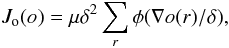 (8)where
φ(x) = |x| − ln(1 + |x|)
and where
∇o(r) = [∇xo2(r) + ∇yo2(r)] 1/2.
Here, ∇xo and
∇yo are the object finite-difference
gradients along x and y, respectively. Equation (8) is effectively
L2 − L1 since it adopts the form
φ(x) ≈ x2/2
when x is close to 0 and
φ(x)/|x| → 1
when x tends to infinity. The global factor μ and the
threshold δ are two hyperparameters that must be adjusted by hand
according to the level of noise and the object structure. Some steps toward semi-automatic
setting of these parameters were made by Blanco &
Mugnier (2011).
(8)where
φ(x) = |x| − ln(1 + |x|)
and where
∇o(r) = [∇xo2(r) + ∇yo2(r)] 1/2.
Here, ∇xo and
∇yo are the object finite-difference
gradients along x and y, respectively. Equation (8) is effectively
L2 − L1 since it adopts the form
φ(x) ≈ x2/2
when x is close to 0 and
φ(x)/|x| → 1
when x tends to infinity. The global factor μ and the
threshold δ are two hyperparameters that must be adjusted by hand
according to the level of noise and the object structure. Some steps toward semi-automatic
setting of these parameters were made by Blanco &
Mugnier (2011).
The regularization term for the PSF, which introduces the myopic criterion into
Eq. (6), assumes that the PSF is a multidimensional Gaussian
random variable. This assumption is justified when one deals with long exposures, which
are, by definition, sums of large numbers of short-exposures. As such they are Gaussian
according to the central limit theorem. Adopting these conditions,
Jh(h) has the form
![Mathematical equation: \begin{equation} J_h({h}) = \dfrac{1}{2} \sum_{f} \dfrac {|{{H}}(f) - {{H}_{m}}(f)|^2}{E[|{{H}}(f) - {{H}_{m}}(f)|]^2}\cdot \label{eq40} \end{equation}](/articles/aa/full_html/2013/07/aa19489-12/aa19489-12-eq60.png) (9)This prior is expressed
in the Fourier domain. The term
Hm(f) = E [H]
is the mean transfer function and
E [| H(f) − Hm(f) |] 2
is the associated power spectral density (PSD) with f denoting spatial
frequency. This Fourier-domain prior bears some resemblance to Eq. (7). Indeed, it also assumes Gaussian statistics
and draws the solution, in the least-squares fashion, toward the user-supplied mean PSF
while obeying the error bars given by the PSD (which give the variance at each frequency).
The PSF prior leads to band-limitedness of the PSF estimate because the ensemble average
in the denominator,
E [| H(f) − Hm(f) |] 2,
should be zero above the diffraction-imposed cut-off.
(9)This prior is expressed
in the Fourier domain. The term
Hm(f) = E [H]
is the mean transfer function and
E [| H(f) − Hm(f) |] 2
is the associated power spectral density (PSD) with f denoting spatial
frequency. This Fourier-domain prior bears some resemblance to Eq. (7). Indeed, it also assumes Gaussian statistics
and draws the solution, in the least-squares fashion, toward the user-supplied mean PSF
while obeying the error bars given by the PSD (which give the variance at each frequency).
The PSF prior leads to band-limitedness of the PSF estimate because the ensemble average
in the denominator,
E [| H(f) − Hm(f) |] 2,
should be zero above the diffraction-imposed cut-off.
In practice, Eq. (9) relies on the availability of several PSF measurements. The mean PSF and its PSD are estimated by replacing the expected values (E [.] ) by an average computed on a PSF sample. When such a sample of several PSFs is not available, as we have assumed in our work, then Hm is made equal to the Fourier transform of the single supplied PSF, and E [| H(f) − Hm(f) |] 2 is computed as the circular mean of |Hm|2. These relatively large error bars are intentional: they account for the lack of knowledge about the PSD when given only a single PSF measurement.
In the original MISTRAL paper (Mugnier et al. 2004) the code was presented mainly in the context of planetary images, for which the object prior (Eq. (8)) was developed. The experimental data presented therein were obtained on several AO systems and covered a wide range of celestial objects such as Jupiters satellites Io and Ganymede and the planets Neptune and Uranus. MISTRAL was applied to the study of the asteroids Vesta (Zellner et al. 2005) and 216-Kleopatra (Hestroffer et al. 2002), and was also used to monitor surface variations on Pluto over a 20-year period (Storrs & Eney 2010).
2.4. IDAC
Multiframe blind deconvolution (MFBD; Schulz 1993; Jefferies & Christou 1993) is an image reconstruction method relying on the availability of several images of an object. In addition, many of the MFBD algorithms rely on short exposures. This was originally dictated by the notion that in imaging through turbulence short-exposure images contain diffraction-limited information while the long exposures do not (Labeyrie 1970). Before the advent of AO the only way to obtain diffraction-limited data from the ground was to record short exposures that could then be processed by one of several “speckle imaging” methods (Knox & Thompson 1974; Lohmann et al. 1983). Therefore, MFBD was originally proposed in the context of speckle imaging.
The MFBD code we used in this paper is called IDAC, for iterative deconvolution algorithm in C 2, and is an extension of the iterative blind deconvolution (IBD) algorithm proposed by Lane (1992). IDAC performs deconvolution by numerically minimizing a functional that is composed of four constraints:  (10)where
 ![Mathematical equation: \begin{equation} E_{\rm im} = \sum_{r\in \gamma}[\hat{o}(r)]^2 + \sum_{i=1}^{M}\sum_{r\in \gamma} [\hat{h}_{i}(r)]^2\label{eq60} \end{equation}](/articles/aa/full_html/2013/07/aa19489-12/aa19489-12-eq68.png) (11)is the image domain error that penalizes the presence of negative pixels (γ) in both the object (o) and the PSF (h) estimates. The subscript i refers to an individual data frame.
(11)is the image domain error that penalizes the presence of negative pixels (γ) in both the object (o) and the PSF (h) estimates. The subscript i refers to an individual data frame.
The so-called convolution error is  (12)which quantifies the fidelity of the reconstruction (Ô) to the data (I) in the Fourier domain. The term Bi is a binary mask that penalizes frequencies beyond the diffraction-imposed cut-off, N2 is a normalization constant where N is the number of pixels in the image.
The third constraint is called the PSF band-limit error and is defined as  (13)It prevents the PSF estimates from converging to a δ function and the object estimate from converging to the observed data. The term
  is a binary mask that is unity for spatial frequencies greater than 1.39 times the cut-off frequency and zero elsewhere.
The last constraint is the Fourier modulus error: ![Mathematical equation: \begin{equation} E_{\rm Fm} = \dfrac{1}{N^2} \sum_{f} \left[|\hat{O}(f)|-|{O}_{\rm e}(f)|\right]^2 \Phi(f), \label{eq75} \end{equation}](/articles/aa/full_html/2013/07/aa19489-12/aa19489-12-eq79.png) (14)where Oe is a first estimate of the Fourier modulus of the object obtained, e.g., from Labeyrie’s speckle interferometry method (Labeyrie 1970), and Φ is a signal-to-noise (SNR) filter. Jefferies & Christou (1993) showed with several simulations that this constraint is especially important since it incorporates relatively high SNR information from a complete dataset formed by many frames. On the other hand, the Fourier modulus of an object is only recoverable directly if one has a set of speckle images of an unresolved source to be used as a reference. There are workarounds to this problem, most notably reference-less approaches reported in Worden et al. (1977) and von der Lühe (1984), but these solutions are applicable only to non-compensated imaging and could not be used in our tests.
(14)where Oe is a first estimate of the Fourier modulus of the object obtained, e.g., from Labeyrie’s speckle interferometry method (Labeyrie 1970), and Φ is a signal-to-noise (SNR) filter. Jefferies & Christou (1993) showed with several simulations that this constraint is especially important since it incorporates relatively high SNR information from a complete dataset formed by many frames. On the other hand, the Fourier modulus of an object is only recoverable directly if one has a set of speckle images of an unresolved source to be used as a reference. There are workarounds to this problem, most notably reference-less approaches reported in Worden et al. (1977) and von der Lühe (1984), but these solutions are applicable only to non-compensated imaging and could not be used in our tests.
While MFBD algorithms were initially proposed in the context of speckle imaging, there is nothing preventing their application to long-exposure AO images that now contain diffraction-limited frequencies. In principle, there are some inherent advantages of working with M frames instead of using a single, co-added long exposure. The multiframe approach reduces the ratio of unknowns to measurements from 2:1 in single-image blind deconvolution to M + 1:M in multi-frame deconvolution. On top of the PSF band-limit constraint (Eq. (13)), concurrent processing of many frames means that the PSF cannot converge to the δ function (this would have yielded an object equal to the data, but the data are generally temporally variable while the object is assumed to be constant in MFBD, which is a good assumption in the context of astronomical imaging on short time-scales). MFBD algorithms are very successful in the case of strongly varying PSFs so that the target is easily distinguished from the PSFs. On the other hand, the goal of AO is to stabilize the PSF. This implies less PSF diversity from one observation to another, so that other constraints become more useful.
The code IDAC can be regarded as a precursor but also a representative of a wider class of MFBD algorithms. We mention here the PCID code (Matson et al. 2009), which has the capability to estimate the PSFs either pixel by pixel in the image domain or in terms of a Zernike-based expansion of the phase in the pupil of the telescope. It has been shown that such a PSF re-parameterization leads to object estimates that are less noisy and have a higher spatial resolution (Matson & Haji 2007).
IDAC was applied to speckle observations of the binary system Gliese 914, and in the process, the secondary component was resolved into two stars (Jefferies & Christou 1993). Additionally, IDAC was one of the five codes used in our study of photometric accuracy of image reconstruction algorithms (Gladysz et al. 2010).
3. Dataset description and methodology
3.1. Dataset description
The images we used to test the algorithms correspond to observations performed with the fourth detector of the WFPC2 camera (Trauger et al. 1994) (the so-called planetary camera -PC-, with a pixel size of 0.046′′) installed on the HST. These are pictures of Saturn (the whole planet is visible) with a dynamic range of up to 975 counts, and galaxy M100 with a peak signal of 7400 counts. To obtain well-defined edges and transitions between the object and the background, the image of Saturn was preprocessed so that all pixels below a certain threshold were set to zero, thus enhancing the visibility of the Cassini and Encke divisions. These images were considered representations of the true objects (Fig. 1).
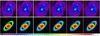 |
Fig. 1 Top, far left: M100 galaxy “ground truth” image. Bottom, far left: Saturn “ground truth” image. From left to right: blurred simulated images using a science PSF with a Strehl ratio = 53% (far left panel in Fig. 2) plus additive Gaussian noise with standard deviations equal to 1, 5, 10, 15, and 20. Linear scale. |
The “ground truth” images were subsequently convolved with an AO PSF with an SR equal to 53% (see Table 1). This and the other PSFs used in this project were obtained with the 1024 × 1024 PHARO infrared camera (Hayward et al. 2001) on the 5-m Hale telescope at the Palomar Observatory (Troy et al. 2000). Closed-loop images of single stars were recorded using the 0.040′′ pixel-1 mode. The images were cropped to size 150 × 150 pixels, which corresponds to a field of view (FOV) of 6′′. The observations were acquired in the K band (2.2 μm) where the diffraction limit is 0.086′′ so that the data meet Nyquist-sampling requirements. The filter of the observations was Brackett Gamma (BrG) and each of the PSFs in Table 1 corresponds to a sum of 200 frames, each with an exposure time of either 1416 or 2832 ms. The individual frames were registered via iterative Fourier shifting to produce shift-and-add images (Baena Gallé & Gladysz 2011).
PSFs used for the simulated observations.
The angular size on the sky over which the AO PSF can be assumed to be almost spatially invariant is the so-called isoplanatic angle. This parameter becomes larger at longer wavelengths. As specified by Hayward et al. (2001), the isoplanatic angle is approximately 50′′ in K-band at Palomar. The angular size of the Saturn and M100 images is 20.5′′, so we can assume that the PSF remains constant throughout the FOV. The difference in pixel scales between those images and the PSFs from Palomar is very small (0.046′′ vs. 0.040′′) and therefore we did not re-bin the images to match their pixel scales. The paper is devoted to comparing image-restoration algorithms and not to the performance evaluation of the AO system at Palomar.
We used IDAC in the multi-frame mode. One of the goals of our work was to check the trade-off between the diversity provided by more frames vs. SNR per frame. One can think of this as an exposure-time optimization. For a constant total observation time per object one can use shorter exposures and hope to exploit the PSF variability in subsequent image restoration with MFBD, or opt instead to use fewer images with a better SNR per frame. Therefore, out of the original 200-frame dataset we have produced datasets of 10, 20, 50, and 100 binned PSFs. These binned PSFs, together with the original 200-frame dataset, were used as blurring kernels for the Saturn image. For AWMLE, ACMLE, and MISTRAL, which are single-image restoration codes, we only used the summed PSF. All PSFs were normalized to have a total power equal to unity before the convolution procedure.
The blurred observations were subsequently corrupted with noise. We explored more than twenty levels of noise: pure Gaussian readout noise of standard deviation ranging from σ = 1 to σ = 20, and shot noise plus readout noise of level σ = 10. These levels correspond to the noise that was added to the summed images. For MFBD with IDAC we worked with several images and decided to add to each frame the amount of noise that would result in the same SNR per summed image had the images been summed and then processed, as in the case of the other three algorithms. This means adding pure Gaussian noise with levels from  to
to  , and Poisson noise plus
  to the 50-frame dataset, for example. This way we aimed to test the benefits of exploiting PSF diversity vs. higher noise per frame, as mentioned above.
One of the goals of the project was to test the susceptibility of the algorithms to mismatch between the science and calibration PSFs. Therefore, we used a matched PSF (SR = 53%), a mismatched PSF (SR = 45%), and a highly mismatched PSF (SR = 36%) as inputs to AWMLE, ACMLE, MISTRAL, and MFBD. The last SR value corresponds to half of the maximum SR in K band (63%) predicted in simulations for the AO system in Palomar (Hayward et al. 2001). Table 1 lists the PSFs used in the tests. Differences in SR for the same star arise because of the changing seeing. All PSFs used in the simulations are presented in Fig. 2.
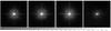 |
Fig. 2 Far left: science PSF with the Strehl ratio (SR) = 53%. Middle left: reference PSF with SR = 53%. Middle right: reference PSF with SR = 45%. Far right: reference PSF with SR = 36%. The far left PSF was used to blur the HST images of Saturn and M100. The other three PSFs were used as reference PSFs for the algorithms. Logarithmic scale. |
3.2. Methodology
The four algorithms are very different and require different strategies to obtain the final result. For AWMLE and ACMLE, it is convenient (although not mandatory) to perform an initial decomposition of the dataset, either in the wavelet or in the curvelet domain. This can give the user an idea as to the number of planes to use during the deconvolution process. Additionally, this preliminary decomposition could inform the user whether it is sensible to perform deconvolution in the highest-frequency plane where the finest structures together with noise have been classified. When working in these planes there is a trade-off between the benefit of recovering information from the finest wavelet/curvelet plane and the undesirable reconstruction of non-significant structures. Both transforms, WT and CT, can also be combined into a dictionary of coefficients (Fadili & Starck 2006), although for the sake of simplicity we executed them independently.
The main difficulty when using a Richardson-Lucy-type algorithm is determining at which iteration to stop the deconvolution process. In AWMLE and ACMLE, this problem is solved by probabilistic masks. The mask can apply significance thresholds to a given location in a given plane to selectively deconvolve statistically similar regions. This concept is called multiresolution support (Starck et al. 2002b). Probabilistic masks are used to stop the deconvolution process automatically in parts of the image where significant structures cannot be discerned. To estimate the value of the mask at a particular location, a local window must be defined. Here we used a window based on the local standard deviation computed within that window: 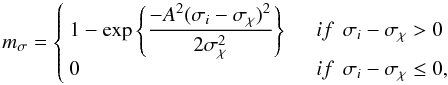 (15)with
 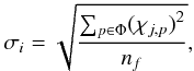 where A is a coefficient for determining the applied threshold, σi is the standard deviation within the window Φ centered on pixel i of the plane χj (pixels within that window are indexed with p), nf is the number of pixels contained in the window, and σχ is the global standard deviation in the corresponding wavelet or curvelet plane. The value for σχ can be determined by decomposing an artificial Gaussian noise image, with standard deviation equal to that in the dataset, into wavelet or curvelet coefficients. These windows are then shifted across all wavelet or curvelet planes to build the final probabilistic mask M (see Eqs. (3) and (5)).
Each of the wavelet planes has the same size as the original image (i.e., 512 × 512). For cases like this, Otazu (2001) proposed to increase the size of the local window mσ with the wavelet scale. The lower the frequency of the representation, the larger the window. Therefore, the window size for the highest-frequency scale was set to 5 × 5, next plane was analysed with a 7 × 7 window, and the third one with a window of size 11 × 11. On the other hand, the curvelet transform decreases the scale, or wedge size, with the scale of representation. For instance, wedges at the highest-frequency scale have a size of 267 × 171 pixels, whereas wedges at a lower-frequency scale can have dimensions of 71 × 87, according to the level of detail being represented. The ratio between dimensions in a given wavelet plane and the corresponding curvelet wedge is between 2 and 3. To closely compare between WT and CT, we kept the same ratio for the window sizes used at each scale for both ways of representation, and a constant window size (3 × 3 pixels) was chosen for the CT. The residual wavelet and curvelet scales were never thresholded, i.e., masks were set to 1 for these scales. Finally, parameter A was set to 3/2 so the window was approximately equal to 1 when σi − σχ = 2σχ, i.e., when coefficients above twice the noise level are detected.
In our experiments we noticed that the results could be improved by changing the values of A and the window sizes, especially for CT. Improvement means here fewer elongated artifacts. On the other hand, for the purpose of a clear and fair comparison between WT and CT, we preferred to keep the values given above, bearing in mind the original decision adopted for AWMLE in Otazu (2001). In our opinion, a more thorough study of the best choices for the parameters of the probabilistic masks is necessary, and in particular, a study in which choices are better suited for a particular way of representation.
The CurveLab software, which was used here to introduce the CT into ACMLE, can perform digital curvelet decomposition via two different implementations. The first one is the so-called USFFT digital CT and the second one is known as the digital CT via wrapping. Both differ in the way they handle the grid that is used to calculate the FFT to obtain the curvelet coefficients. This grid is not defined in typical Cartesian coordinates, instead, it emulates a polar representation, more suited to the mathematical framework defined in Candès et al. (2006). The USFFT version has the drawback of being computationally more intensive than to the wrapping version, since the latter makes a simpler choice of the grid to compute the curvelets (Starck et al. 2010). Hence, for reasons of computational efficiency, the wrapping version was used in ACMLE.
The user has to provide CurveLab with the values of some parameters. In addition to the number of curvelet scales, the number of orientations or angles of representation in the second scale is also required as input from the user. This parameter will automatically set the number of angles for the rest of the scales. Evidently, the higher the number of orientations, the longer the algorithm will need to perform CT, the higher the overall redundancy and the higher the computational cost for calculating the probabilistic masks at each scale. We decided to set this parameter to 16 as a trade-off between having a complete representation of all possible orientations in the image and the total execution time. Finally, a third parameter decides if the curvelet transform is replaced by an orthogonal wavelet representation at the final scale, i.e., the highest-frequency scale. In our experiments we saw no significant differences between results based on one choice for this parameter’s value or the other.
MISTRAL performs the minimization process of Eq. (6) by the partial conjugate-gradient method. The code requires that the user provides values for the hyperparameters μ and δ (see Eq. (8)), which balance the smoothing imposed by too much regularization against noise amplification. This has to be done by trial and error although the authors of the algorithm provide some suggestions in the original MISTRAL paper, namely that μ be set to around unity and δ be set to the norm of the image gradient (∥ ∇i ∥ = [∑ p|∇i(p)|2] 1/2). In practice, the user experiments with various values of these parameters, and chooses the image reconstruction that is most visually appealing. In our tests we found that μ = 10 and δ = 2 yielded the best results. We let the code run for the maximum number of iterations set to 103.
IDAC requires the user to provide the value of the diffraction-limit cut-off. Caution should be taken here: the code requires that all supplied images are of the same dimensions. Therefore, when one has a PSF image that is smaller in size than the science image, the PSF should be embedded in an array of zeros. Subsequently, the diffraction-limit cut-off should be estimated from the zero-padded, and not the original Fourier-transformed PSF (see Fig. 3). Another parameter that should in theory affect the restorations, a scalar quantifying user confidence in the supplied PSF, was found to have negligible effect on the outputs.
As with MISTRAL, we let the code run for the maximum number of iterations set to 103. For images with a high level of noise (Gaussian σ ≥ 10 and Poisson noise plus Gaussian σ = 10) it converged quickly, after 15 − 20 iterations, which can be considered a good behavior because the noise did not become amplified. For cases with low noise (σ ≤ 5) the algorithm converged after 50 − 100 iterations and produced generally sharper reconstructions.
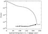 |
Fig. 3 Normalized power spectrum of the 53% SR PSF (Fig. 2 middle left). The diffraction- and noise-limited cut-off frequency was determined to be approximately 230 pixels. The PSF was embedded in an array of zeros to match the size of the science image (512 × 512 pixels). |
4. Quality metrics and maps
One of the goals of this work was to compare the quality of reconstructions yielded by several codes. Therefore, metrics were needed for image quality assessment. Here we have chosen the mean squared error (MSE), which is probably the most commonly used metric in image processing (e.g. Mugnier et al. 2004) and one of the oldest and most often used metrics to evaluate the resemblance of two images. It is defined as  (16)where, in this context, M is the total number of pixels in the image and x and y are pixel values of the two images that are compared. It is also very common to use the related metric, the peak signal-to-noise ratio (PSNR), defined as
  (17)where L is the dynamic range of the image. These metrics are very easy to compute and measure the pixel-by-pixel departure between the reconstruction and the reference object. The MSE and PSNR have a clear physical meaning: they quantify the energy of the error. Hence, they are well suited to the task of estimating the absolute photometric error between the two images.
We preferred to use PSNR rather than MSE to quantify differences between images, since the former has the more intuitive behavior of setting higher values to better reconstructions. We set L = 975 in Eq. (17) to match the dynamic range of the “ground truth” Saturn object, and L = 7400 to match the maximum value present in the original image of M100, which corresponds to the galaxy core. A difference in 1 dB in PSNR implies an approximate difference between 150 and 250 in MSE, depending on the object.
In what follows we also show the so-called error and residual maps. When one obtains a certain reconstruction after solving the main image formation equation (Eq. (2))  (18)where ô is the reconstruction or solution found with a certain algorithm, the error map is the exact difference between the “ground truth” object and the reconstruction, i.e., e = o − ô. It offers a detailed, pixel-by-pixel or structure-by-structure, view of the algorithm’s performance. Unfortunately, in practical situations the real object is not available, so the reconstruction error measurement is usually made in the image domain by transferring the solution ô into the image domain by means of the PSF h, and subtracting it from the data. Hence, the normalized residual map is computed as
  (19)In the case of static-PSF approaches, h is the input calibrator, whereas for myopic- and blind-approaches h is the PSF estimate found in the last iteration. The residual map is a graphical comparison in the image domain meant to show how close, from a mathematical point of view, the reconstruction and the data are to each other. On the other hand, the error map is a more truthful comparison, from a physical point of view, of the solution and the (usually unknown) reality.
5. Results and discussion
The tests were conducted decomposing Saturn and M100 datasets into three wavelet/curvelet planes plus a wavelet/ curvelet residual. As mentioned before, three levels of mismatch between the science and calibration PSF were analyzed, as well as twenty levels of noise, including readout and shot noise. All outputs were analyzed by means of the PSNR metric.
Figures 4 and 5 show the evolution of the PSNR metric with respect to the level of noise when a mismatch of ~8% in SR exists between the science and the reference PSF. Apart from the logical conclusion that reconstruction quality decreases as the noise increases, we can point out that firstly, despite of being designed for detecting elongated structures, ACMLE performs reasonably well in low-noise-level conditions for an image where many point-like sources are present such as M100 (Fig. 4). Only when the noise level reaches a value of σ ~ 8 and the correlation of information along lines and edges has significantly deteriorated, its performance becomes comparable to that of AWMLE. This effect does not happen for the Saturn image (Fig. 5) where almost all information is distributed along elongated features and the curvelet transform is more resistant against noise. Secondly, myopic- and blind-PSF algorithms show a more evident deterioration of performance with the increasing level of noise. For MISTRAL, its performance for low-level-noise conditions is extremely good for Saturn, whereas it becomes similar to static-PSF algorithms with noise control at a level of σ = 12. This is basically due to its good behavior at the edges of the planet thanks to the L2 − L1 prior included in the code. The rest of algorithms exhibit evident Gibbs oscillations in the high transitions between the planet limits and the background. When these edges were not considered in the computation of PSNR, MISTRAL’s performance evolution for Saturn with respect to other algorithms has a similar behavior to that shown for galaxy M100 in Fig. 4. It has to be mentioned, though, that MISTRAL was developed specifically in the context of imaging planetary-type bodies and its prior is not very suitable for galaxies or stellar fields, for which a white spatial prior, which assumes independency between pixels, is more advisable (Ygouf et al. 2013). On the other hand, including these regularization terms could potentially improve results obtained with MFBD and AW(C)MLE.
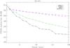 |
Fig. 4 PSNR evolution of M100 reconstructions with respect to the level of noise. Blurred simulated images were corrupted with Gaussian noise with standard deviations ranging from σ = 1 to σ = 20. All reconstructions used the SR = 45% PSF as the calibrator. Pink squares: ACMLE. Blue crosses: AWMLE. Green diamonds: MISTRAL. Black triangles: MFBD. |
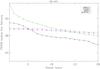 |
Fig. 5 PSNR evolution of Saturn reconstructions with respect to the level of noise. Blurred simulated images were corrupted with Gaussian noise with standard deviations ranging from σ = 1 to σ = 20. All reconstructions used the SR = 45% PSF as the calibrator. Pink squares: ACMLE. Blue crosses: AWMLE. Green diamonds: MISTRAL. Black triangles: MFBD. |
As mentioned in Sect. 3.1, datasets of 10, 20, 50, and 100 binned images, together with the original 200-frame dataset, were used as input for IDAC to test the trade-off between the (implied) PSF diversity and SNR per frame. We tried to shed some light on the question which of the following strategies is better: deconvolving a long-exposure image with a relatively high SNR (AWMLE, ACMLE and MISTRAL algorithms), or tackling the problem by dividing the dataset into more (diverse) frames at the expense of reducing the SNR for each frame (MFBD). It was found that the original 200-frame set yielded significantly poorer results than the smaller sets. Specifically, the 50-frame dataset proved to be the best input to IDAC although the differences between its output and those of the 10- and 20-frame sets were small. For the data sets we used, there is no evidence that the higher diversity provided by more frames yields better results. Therefore, we conclude that (assuming constant total observation time) using very short exposure times is not the best solution for MFBD, when used after AO, because relatively low PSF diversity does not offset the high level of relative noise per frame. Figures 4 and 5 show that MFBD behaves in a similar way as the other algorithms for low-noise-level conditions, but its performance is highly affected as the noise per frame increases.
Figures 6 and 7 reveal how the algorithms behave with respect to the mismatch between the calibrator and the science PSF for different levels of noise (σ = 1, 10 and 20 as well as shot noise plus read-out noise of σ = 10). In general, static-PSF approaches yield better reconstructions than myopic- and blind- codes when the two PSFs agree well. For M100 the advantage of ACMLE with respect to MISTRAL is around 3 − 5 dB, while it is higher than 5 dB with respect to IDAC for noise levels above σ = 10. For the Saturn image the results are similar except for low-noise-level conditions where L2 − L1 prior gives MISTRAL an advantage. A mismatch of ~8% in SR does not lead to large differences in the results of the algorithms (Figs. 6 and 7, middle rows), with respect to those obtained with a well-matched reference PSF (same figures, top rows). A reference PSF with SR = 36%, which implies a mismatch of ~17% SR, can be seen to have a more noticeable effect on the static-PSF codes and, surprisingly, MFBD than on MISTRAL (Figs. 6 and 7, bottom rows). The reconstruction quality for MISTRAL is more uniform as a function of PSF mismatch, which is a logical result since this algorithm is designed to deal with large differences between the science and the reference PSFs. At this level of mismatch there is already a visible qualitative difference between the PSFs (compare the leftmost and rightmost panels of Fig. 2), which affects the performance of static-PSF codes. We stress that, although MISTRAL is very robust to PSF mismatch, its advantages become highly attenuated as the noise level increases. This can be clearly seen in Fig. 6, bottom row, noise level of σ = 20. This shows that the ability of a method to control the noise is as critical as its capability to update the PSF.
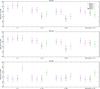 |
Fig. 6 Each plot shows the mean value and standard deviation of the PSNR metric calculated from M100 results obtained with ACMLE (pink squares), AWMLE (blue crosses), MISTRAL (green diamonds), and MFBD (black triangles). Deconvolution was performed with three PSFs to represent different levels of miscalibration. Top row: dataset was deconvolved with a matched PSF (SR = 53%). Middle row: dataset was deconvolved with a mismatched PSF (SR = 45%). Bottom row: dataset was deconvolved with a highly mismatched PSF (SR = 36%). |
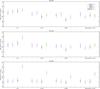 |
Fig. 7 Each plot shows the mean value and standard deviation of the PSNR metric calculated from Saturn results obtained with ACMLE (pink squares), AWMLE (blue crosses), MISTRAL (green diamonds), and MFBD (black triangles). Deconvolution was performed with three PSFs to represent different levels of miscalibration. Top row: dataset was deconvolved with a matched PSF (SR = 53%). Middle row: dataset was deconvolved with a mismatched PSF (SR = 45%). Bottom row: dataset was deconvolved with a highly mismatched PSF (SR = 36%). |
Figures 8 and 9 show the reconstructions of M100 achieved by the algorithms for the noise levels of σ = 5 and σ = 15 and a mismatch of ~8% in SR. ACMLE yielded the sharpest reconstruction, although some elongated artifacts start to become visible at σ = 15 as a result of an incorrect identification of the coefficients. Compared to MISTRAL, both ACMLE and AWMLE are able to enhance and de-blend from the surrounding cloud more individual point-like sources. MFBD reconstructions are still almost as smooth as the starting image. Figures 10 and 11 show the results for Saturn. Here, similar conclusions can be formulated, i.e., noise amplification is better controlled by AW(C)MLE thanks to the multiresolution support. AWMLE and ACMLE exhibit the best results in the planet’s body (in terms of the achieved resolution and noise attenuation), and also in the background space between Saturn’s body and the innermost ring, which is a measure of a given algorithm’s ability to suppress noise. This effect is also visible in Cassini’s division. Furthermore, Encke’s division is barely visible in MISTRAL’s and MFBD’s reconstructions for high noise level of σ = 15. On the other hand, AWMLE, ACMLE, and MFBD show the typical ringing effect associated with strong transitions or edges (very visible at the limits of Saturn’s body), whereas MISTRAL’s L2 − L1 edge-preserving prior attenuates these effects considerably. Nevertheless, this prior must be responsible for the excessive attenuation of some elongated features present in Saturn’s inner ring that were detected with ACMLE, AWMLE, and MFBD, although over-reconstructed by the former and noise-distorted by the latter two. We stress that such features are not visible in the blurred and corrupted image.
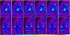 |
Fig. 8 Column A: M100 original image. Column B: degraded and corrupted image with Gaussian noise (σ = 5). Column C: ACMLE reconstruction. Column D: AWMLE. Column E: MISTRAL. Column F: MFBD. Top row: whole view. Bottom row: view of representative detail. Reconstructions were performed with a reference PSF at SR = 45%. Linear scale from 0 to 1000. |
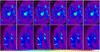 |
Fig. 9 Column A: M100 original image. Column B: degraded and corrupted image with Gaussian noise (σ = 15). Column C: ACMLE reconstruction. Column D: AWMLE. Column E: MISTRAL. Column F: MFBD. Top row: whole view. Bottom row: view of representative detail. Reconstructions were performed with a reference PSF at SR = 45%. Linear scale from 0 to 1000. |
Finally, we show in Figs. 12 and 13 the error and residual maps. For the Saturn image, one can see that ACMLE’s and AWMLE’s results have values closer to the truth in all pixels of the object (planet’s body, space between the body, and the innermost ring), except in the pixels at the edges of the main planet body and the rings, which show poor numbers. For these pixels, L2 − L1 object prior implemented in MISTRAL is working impressively well, while MFBD, ACMLE, and AWMLE’s values strongly depart from the real object. In general, the latter three algorithms have the tendency to over-reconstruct bright sources and bright structures of the image, while MISTRAL exhibits the opposite behavior, i.e., it does not reach the correct photometric value for these regions. Noise amplification or lack of noise suppression is evident for MFBD and MISTRAL, whereas some elongated artificial structures are visible in ACMLE’s result, thus showing an incorrect coefficient identification at some orientations. This suggests that the probabilistic mask should not be applied to each curvelet wedge and scale independently, as we do in this work, but creating some mechanism to exchange information among them. There are no significant differences in the residual maps obtained by ACMLE and MISTRAL (Fig. 13) apart of those already mentioned, although here they are not as evident as in the error maps. This suggests that updating the PSF in MISTRAL yields a mathematical solution that is compatible with the data as in the case of AW(C)MLE. However, when the noise increases, the regularization term in MISTRAL does not provide as good results as the AW(C)MLE, even if MISTRAL updates the PSF.
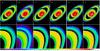 |
Fig. 10 Column A: Saturn original image. Column B: degraded and corrupted image with Gaussian noise (σ = 5). Column C: ACMLE reconstruction. Column D: AWMLE. Column E: MISTRAL. Column F: MFBD. Top row: whole view. Bottom row: view of representative detail. Reconstructions were performed with a reference PSF at SR = 45%. Linear scale from 0 to 1000. |
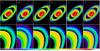 |
Fig. 11 Column A: Saturn original image. Column B: degraded and corrupted image with Gaussian noise (σ = 15). Column C: ACMLE reconstruction. Column D: AWMLE. Column E: MISTRAL. Column F: MFBD. Top row: whole view. Bottom row: view of representative detail. Reconstructions were performed with a reference PSF at SR = 45%. Linear scale from 0 to 1000. |
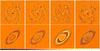 |
Fig. 12 Error maps for the reconstructions obtained from data sets corrupted with Gaussian noise with σ = 5. Reconstructions were performed with a reference PSF at SR = 45%. Column A: ACMLE. Column B: AWMLE. Column C: MISTRAL. Column D: MFBD. Linear scale from − 100 to 100. |
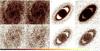 |
Fig. 13 Residual maps for the reconstructions obtained from data sets corrupted with Gaussian noise with σ = 5 (top row) and σ = 15 (bottom row). Reconstructions were performed with a reference PSF at SR = 45%. Columns A and C: ACMLE. Columns B and D: MISTRAL. Linear scale from 0 to 1. |
6. Conclusions
We have introduced a way of using the multiresolution support, applied in the wavelet and curvelet domain, in the post-processing of adaptive-optics images to help control the process of noise amplification. One of the most important goals of this research was to devise an objective check of the typical assumption (within the AO astronomical community) about the supposed poor performance of static-PSF approaches with respect to the blind/myopic methods. For the dataset we used, the Richardson-Lucy scheme, which is controlled over the wavelet- or curvelet domain by a σ-based mask, provided a very competitive performance against the more well-known approaches like MFBD or regularized deconvolution (MISTRAL). Specifically, it yielded 3 − 5 dB better results (in terms of PSNR) than IDAC and MISTRAL for a mismatch in the PSF of up to 8% in terms of the Strehl ratio. On the other hand, performance of MISTRAL was photometrically better when highly mismatched PSF of SR = 36% (mismatch of 17% in SR) was employed as calibrator.
We showed that probabilistic masks can control noise amplification in a Richardson-Lucy scheme, and also that curvelet transform (CT) performs better than wavelet transform (WT) for low-noise-level conditions, when elongated structures and edges still keep their bidimensional characteristics above the noise level.
The observed poor performance of IDAC, which can be visually appreciated in Figs. 9 − 11, can be explained in the following way. Multiframe approaches rely on diverse PSFs to separate the blurring kernel from the object and to make the blind problem more tractable (less under-determined). Having more images helps when one has truly diverse PSFs. But this is not always the case with AO imaging. In fact, AO will stabilize the PSF and no number of new frames can then supply new information for MFBD. The standard deviation of the Strehl ratio value across the 200 frames used as input for IDAC was only 2%. For all datasets that we had (ten stars), the standard deviation across 200 frames rarely exceeded 5%. It seems that single-image codes like MISTRAL or AW(C)MLE have an advantage in the case of stable AO observations.
Several lines of research are still open. It would be possible to study other types of masks, such as those based on the quadratic distance between related zones in consecutive wavelet planes (Starck & Murtagh 1994) or image segmentation (or wavelet plane segmentation) by means of neural networks to link and classify significant zones in the image (Núñez & Llacer 1998). Furthermore, the use of other wavelet transforms, such as the undecimated Mallat trasform with three directions per scale, and many other multitransforms should be studied and compared, e.g., shearlets (Guo & Labate 2007) or waveatoms (Demanet & Ying 2007), to name only two.
Much more important, in our opinion, is studying how multitransform support or probabilistic masks can be included into blind and myopic approaches to improve their performance in terms of controlling the noise reconstruction inherent to every image reconstruction algorithm. This will be the topic of our future research.
Acknowledgments
We would like to thank Nicholas Law (University of Toronto) for supplying the PSFs from the Palomar Observatory. We extend our gratitude to Xavier Otazu (Universitat Autònoma de Barcelona), Julian Christou (Large Binocular Telescope Observatory) and Laurent Mugnier (ONERA − The French Aerospace Lab) for useful comments and suggestions about the correct usage of algorithms AWMLE, IDAC and MISTRAL, respectively. We would also like to thank our referee, whose suggestions and comments helped us to improve the paper. Effort sponsored by the Air Force Office of Scientific Research, Air Force Material Command, USAF, under grant number FA8655-12-1-2115, and by the Spanish Ministry of Science and Technology under grant AyA-2008-01225. The US Government is authorized to reproduce and distribute reprints for Governmental purpose notwithstanding any copyright notation thereon.
References
- Andrews, H. C., & Hunt B. R. 1977, Digital Image Restoration (New York: Prentice-Hall, Inc., Englewood Cliffs) [Google Scholar]
- Baena Gallé, R., & Gladysz, S. 2011, PASP, 123, 865 [NASA ADS] [CrossRef] [Google Scholar]
- Bertero, M., & Boccacci, P. 1998, Introduction to inverse problems in imaging (London: Inst. Phys.) [Google Scholar]
- Blanco, L., & Mugnier, L.M. 2011, Optics Express, 19, 23227 [Google Scholar]
- Bouman, C., & Sauer, K. 1993, IEEE Trans. Image Proc., 2, 296 [Google Scholar]
- Candès, E., Demanet, L., Donoho, D., & Ying, L. 2005, Multiscale Model. Simul., 5, 861 [Google Scholar]
- Conan, J.-M., Fusco, T., Mugnier, L. M., Kersalé, E., & Michau, V. 1999, Astronomy with adaptive optics: present results and future programs. ESO Conference and Workshop Proc., ed. D. Bonaccini (Germany: Garching bei München), 56, 121 [Google Scholar]
- Demanet, L., & Ying, L. 2007, Appl. Comp. Harmon. Anal., 23, 368 [CrossRef] [Google Scholar]
- Diolaiti, E., Bendinelli, O., Bonaccini, D., et al. 2000, A&AS, 147, 335 [NASA ADS] [CrossRef] [EDP Sciences] [Google Scholar]
- Esslinger, O., & Edmunds, M. G. 1998, A&AS, 129, 617 [NASA ADS] [CrossRef] [EDP Sciences] [Google Scholar]
- Fadili, M. J., & Starck, J. L. 2006, Sparse representation-based image deconvolution by iterative thresholding (France: ADA IV, Elsevier) [Google Scholar]
- Frieden, B. 1978, Image enhancement and restoration (Berlin: Springer) [Google Scholar]
- Gladysz, S., Baena-Gallé, R., Christou, J. C., & Roberts, L. C. 2010, Proc. of the AMOS Tech. Conf., E24 [Google Scholar]
- González Audícana, M.,Otazu, X., Fors, O., & Seco, A. 2005, Int. J. Remote Sensing, 26, 595 [NASA ADS] [CrossRef] [Google Scholar]
- Green, P. J. 1990, IEEE Trans. Med. Imaging, 9, 84 [Google Scholar]
- Guo, K., & Labate, D. 2007, SIAM J. Math Anal., 39, 298 [Google Scholar]
- Hayward, T. L., Brandl, B., et al. 2001, PASP, 113, 105 [NASA ADS] [CrossRef] [Google Scholar]
- Hestroffer, D., Marchis, F., Fusco, T., & Berthier, J. 2002, Res. Note A&A, 394, 339 [NASA ADS] [CrossRef] [EDP Sciences] [Google Scholar]
- Holschneider, M., Kronland-Martinet, R., Morlet, J., & Tchamitchian, P. 1989, Wavelets, Time-Frequency Methods and Phase Space (Berlin: Springer-Verlag) [Google Scholar]
- Knox, K. T., & Thompson, B. J. 1974, ApJ, 193, L45 [NASA ADS] [CrossRef] [Google Scholar]
- Jaynes, J. T. 1982, Proc. IEEE, 70, 939 [NASA ADS] [CrossRef] [Google Scholar]
- Jefferies, S., & Christou, J. C. 1993, ApJ, 415, 862 [NASA ADS] [CrossRef] [Google Scholar]
- Labeyrie, A. 1970, A&A, 6, 85 [NASA ADS] [Google Scholar]
- Lambert, P., Pires, S., Ballot, J., et al. 2006, A&A, 454, 1021 [NASA ADS] [CrossRef] [EDP Sciences] [Google Scholar]
- Lane, R. G. 1992, JOSA A, 9, 1508 [NASA ADS] [CrossRef] [Google Scholar]
- Llacer, J., & Núñez, J. 1990, The restoration of HST images and spectra (Baltimore: STScI) [Google Scholar]
- Llacer, J., Veklerov, E., Coakley, K. J., Hoffman, E. J., & Núñez, J. 1993, IEEE Trans. Med. Imag., 12, no. 2, 215 [Google Scholar]
- Lohmann, A. W., Weigelt, G., & Wirnitzer, B. 1983, Appl. Opt., 22, 4028 [NASA ADS] [CrossRef] [PubMed] [Google Scholar]
- Lucy, L. B. 1974, AJ, 79, 745 [NASA ADS] [CrossRef] [Google Scholar]
- Lucy, L. B. 1994, The restoration of HST images and spectra II (Boston: STScI) [Google Scholar]
- Matson, C. L., & Haji, A. 2007, Proc. of the AMOS Tech. Conf., E80 [Google Scholar]
- Matson, C. L., Borelli, K., Jefferies, S., et al. 2009, Appl. Opt., 48, A75 [NASA ADS] [CrossRef] [Google Scholar]
- Molina, R., Núñez, J., Cortijo, F., & Mateos, J. 2001, IEEE Signal Proc. Magazine, 18, 11 [Google Scholar]
- Mugnier, L. M., Fusco, T., & Conan, J. M. 2004, JOSA A, 21, 1841 [Google Scholar]
- Murtagh, F., Starck, J. L., & Bijaoui, A. 1995, A&AS, 112, 179 [NASA ADS] [Google Scholar]
- Núñez, J., & Llacer J. 1993, PASP, 105, 1192 [NASA ADS] [CrossRef] [Google Scholar]
- Núñez, J., & Llacer, J. 1998, A&AS, 131, 167 [NASA ADS] [CrossRef] [EDP Sciences] [Google Scholar]
- Otazu, X. 2001, Ph.D. Thesis, University of Barcelona, Barcelona, http://www.tesisenred.net/handle/10803/732 [Google Scholar]
- Otazu, X., González Audícana, M., Fors, O., & Núñez, J. 2005, IEEE Trans. on GeoScience and Remote Sensing, 43, 2376 [Google Scholar]
- Richardson, W. H. 1972, JOSA, 62, no. 1, 55 [Google Scholar]
- Schulz, T. J. 1993, JOSA A, 10, 1064 [NASA ADS] [CrossRef] [Google Scholar]
- Shensa, M. J. 1992, IEEE Trans. on Signal Proc., 40, 2464 [Google Scholar]
- Starck, J. L., & Murtagh, F. 1994, A&A, 288, 342 [NASA ADS] [Google Scholar]
- Starck, J. L., Murtagh, F., Querre, P., & Bonnarel, F. 2001, A&A 368, 730 [NASA ADS] [CrossRef] [EDP Sciences] [Google Scholar]
- Starck, J. L., Donoho, D. L., & Candès, E. 2002a, A&A, 398, 785 [Google Scholar]
- Starck, J. L., Pantin, E., & Murtagh, F. 2002b, PASP, 114, 1051 [NASA ADS] [CrossRef] [Google Scholar]
- Starck, J. L., Aghanim, N., & Forni, O. 2004, A&A 416, 9 [NASA ADS] [CrossRef] [EDP Sciences] [Google Scholar]
- Starck, J. L., Murtagh, F., & Fadili, M. J. 2010, Sparse Image and Signal Processing: wavelets, curvelets, morphological diversity (Cambridge: Cambridge University Press) [Google Scholar]
- Storrs, A., & Eney, B. 2010, Bull. Am. Astr. Soc., 42, 456 [NASA ADS] [Google Scholar]
- Thiébaut, E., & Conan, J. M. 1995, JOSA A, 12, 485 [Google Scholar]
- Tikhonov, A. N., Goncharski, A. V., Stepanov, V. V., & Kochiko, I. V. 1987, Sov. Phys. Doklady, 32, 456 [NASA ADS] [Google Scholar]
- Trauger, J. T., Ballester, G. E., Burrows, C. J., et al. 1994, ApJ, 435, L3 [NASA ADS] [CrossRef] [Google Scholar]
- Troy, M., Dekany, R. G., Brack, G. L., et al. 2000, Proc. SPIE, 4007, 31 [Google Scholar]
- von der Lühe, O. 1984, JOSA A, 1, 510 [Google Scholar]
- Worden, S. P., Stein, M. K., Schmidt, G. D., & Angel, J. R. P. 1977, Icarus, 32, 450 [NASA ADS] [CrossRef] [Google Scholar]
- Ygouf, M., Mugnier, L. M., Mouillet, D., Fusco, T., & Beuzit, J.-L. 2013, A&A, submitted [Google Scholar]
- Zellner, N. E. B., Gibbard, S., & de Pater, I. 2005, Icarus, 61, 355 [Google Scholar]
All Tables
All Figures
|
Fig. 1 Top, far left: M100 galaxy “ground truth” image. Bottom, far left: Saturn “ground truth” image. From left to right: blurred simulated images using a science PSF with a Strehl ratio = 53% (far left panel in Fig. 2) plus additive Gaussian noise with standard deviations equal to 1, 5, 10, 15, and 20. Linear scale. |
| In the text | |
|
Fig. 2 Far left: science PSF with the Strehl ratio (SR) = 53%. Middle left: reference PSF with SR = 53%. Middle right: reference PSF with SR = 45%. Far right: reference PSF with SR = 36%. The far left PSF was used to blur the HST images of Saturn and M100. The other three PSFs were used as reference PSFs for the algorithms. Logarithmic scale. |
| In the text | |
|
Fig. 3 Normalized power spectrum of the 53% SR PSF (Fig. 2 middle left). The diffraction- and noise-limited cut-off frequency was determined to be approximately 230 pixels. The PSF was embedded in an array of zeros to match the size of the science image (512 × 512 pixels). |
| In the text | |
|
Fig. 4 PSNR evolution of M100 reconstructions with respect to the level of noise. Blurred simulated images were corrupted with Gaussian noise with standard deviations ranging from σ = 1 to σ = 20. All reconstructions used the SR = 45% PSF as the calibrator. Pink squares: ACMLE. Blue crosses: AWMLE. Green diamonds: MISTRAL. Black triangles: MFBD. |
| In the text | |
|
Fig. 5 PSNR evolution of Saturn reconstructions with respect to the level of noise. Blurred simulated images were corrupted with Gaussian noise with standard deviations ranging from σ = 1 to σ = 20. All reconstructions used the SR = 45% PSF as the calibrator. Pink squares: ACMLE. Blue crosses: AWMLE. Green diamonds: MISTRAL. Black triangles: MFBD. |
| In the text | |
|
Fig. 6 Each plot shows the mean value and standard deviation of the PSNR metric calculated from M100 results obtained with ACMLE (pink squares), AWMLE (blue crosses), MISTRAL (green diamonds), and MFBD (black triangles). Deconvolution was performed with three PSFs to represent different levels of miscalibration. Top row: dataset was deconvolved with a matched PSF (SR = 53%). Middle row: dataset was deconvolved with a mismatched PSF (SR = 45%). Bottom row: dataset was deconvolved with a highly mismatched PSF (SR = 36%). |
| In the text | |
|
Fig. 7 Each plot shows the mean value and standard deviation of the PSNR metric calculated from Saturn results obtained with ACMLE (pink squares), AWMLE (blue crosses), MISTRAL (green diamonds), and MFBD (black triangles). Deconvolution was performed with three PSFs to represent different levels of miscalibration. Top row: dataset was deconvolved with a matched PSF (SR = 53%). Middle row: dataset was deconvolved with a mismatched PSF (SR = 45%). Bottom row: dataset was deconvolved with a highly mismatched PSF (SR = 36%). |
| In the text | |
|
Fig. 8 Column A: M100 original image. Column B: degraded and corrupted image with Gaussian noise (σ = 5). Column C: ACMLE reconstruction. Column D: AWMLE. Column E: MISTRAL. Column F: MFBD. Top row: whole view. Bottom row: view of representative detail. Reconstructions were performed with a reference PSF at SR = 45%. Linear scale from 0 to 1000. |
| In the text | |
|
Fig. 9 Column A: M100 original image. Column B: degraded and corrupted image with Gaussian noise (σ = 15). Column C: ACMLE reconstruction. Column D: AWMLE. Column E: MISTRAL. Column F: MFBD. Top row: whole view. Bottom row: view of representative detail. Reconstructions were performed with a reference PSF at SR = 45%. Linear scale from 0 to 1000. |
| In the text | |
|
Fig. 10 Column A: Saturn original image. Column B: degraded and corrupted image with Gaussian noise (σ = 5). Column C: ACMLE reconstruction. Column D: AWMLE. Column E: MISTRAL. Column F: MFBD. Top row: whole view. Bottom row: view of representative detail. Reconstructions were performed with a reference PSF at SR = 45%. Linear scale from 0 to 1000. |
| In the text | |
|
Fig. 11 Column A: Saturn original image. Column B: degraded and corrupted image with Gaussian noise (σ = 15). Column C: ACMLE reconstruction. Column D: AWMLE. Column E: MISTRAL. Column F: MFBD. Top row: whole view. Bottom row: view of representative detail. Reconstructions were performed with a reference PSF at SR = 45%. Linear scale from 0 to 1000. |
| In the text | |
|
Fig. 12 Error maps for the reconstructions obtained from data sets corrupted with Gaussian noise with σ = 5. Reconstructions were performed with a reference PSF at SR = 45%. Column A: ACMLE. Column B: AWMLE. Column C: MISTRAL. Column D: MFBD. Linear scale from − 100 to 100. |
| In the text | |
|
Fig. 13 Residual maps for the reconstructions obtained from data sets corrupted with Gaussian noise with σ = 5 (top row) and σ = 15 (bottom row). Reconstructions were performed with a reference PSF at SR = 45%. Columns A and C: ACMLE. Columns B and D: MISTRAL. Linear scale from 0 to 1. |
| In the text | |
Current usage metrics show cumulative count of Article Views (full-text article views including HTML views, PDF and ePub downloads, according to the available data) and Abstracts Views on Vision4Press platform.
Data correspond to usage on the plateform after 2015. The current usage metrics is available 48-96 hours after online publication and is updated daily on week days.
Initial download of the metrics may take a while.