| Issue |
A&A
Volume 554, June 2013
|
|
|---|---|---|
| Article Number | A127 | |
| Number of page(s) | 17 | |
| Section | Extragalactic astronomy | |
| DOI | https://doi.org/10.1051/0004-6361/201321192 | |
| Published online | 17 June 2013 | |
HAWK-I infrared supernova search in starburst galaxies⋆
1
Department of Astronomy, Padova University,
Vicolo dell’Osservatorio 3,
35122
Padova,
Italy
e-mail: This email address is being protected from spambots. You need JavaScript enabled to view it.
2
INAF, Osservatorio Astronomico di Padova,
vicolo dell’Osservatorio 5,
35122
Padova,
Italy
3
INAF, Osservatorio Astronomico di Capodimonte,
Salita Moiariello 16,
80131
Napoli,
Italy
4
INAF, Osservatorio Astrofisico di Arcetri, Largo
Enrico Fermi 5, 50125
Firenze,
Italy
5
Departamento de Ciencias Fisicas, Universidad Andrés
Bello, Av. República 252,
8320000
Santiago,
Chile
6
Institut de Ciéncies de l’Espai (IEEC–CSIC), Facultat de
Ciéncies, Campus
UAB, 08193
Bellaterra,
Spain
Received:
30
January
2013
Accepted:
14
March
2013
Abstract
Context. The use of SN rates to probe explosion scenarios and to trace the cosmic star formation history received a boost from a number of synoptic surveys. There has been a recent claim of a mismatch by a factor of two between star formation and core collapse SN rates, and different explanations have been proposed for this discrepancy.
Aims. We attempted an independent test of the relation between star formation and supernova rates in the extreme environment of starburst galaxies, where both star formation and extinction are extremely high.
Methods. To this aim we conducted an infrared supernova search in a sample of local starbursts galaxies. The rationale behind searching in the infrared is to reduce the bias due to extinction, which is one of the putative reasons for the observed discrepancy between star formation and supernova rates. To evaluate the outcome of the search we developed a MonteCarlo simulation tool that is used to predict the number and properties of the expected supernovae based on the search characteristics and the current understanding of starburst galaxies and supernovae.
Results. During the search we discovered 6 supernovae (4 with spectroscopic classification), which is in excellent agreement with the prediction of the MonteCarlo simulation tool that is, on average, 5.3 ± 2.3 events.
Conclusions. The number of supernovae detected in starburst galaxies is consistent with what is predicted from their high star formation rate when we recognize that a major fraction (~ 60%) of the events remain hidden in the inaccessible, high-density nuclear regions because of a combination of reduced search efficiency and high extinction.
Key words: supernovae: general / galaxies: starburst / galaxies: star formation / infrared: galaxies / infrared: stars
ESO proposal: 083.D-0259, 085.D-0335, 085.D-0348, 087.D-0494, 087.D-0922. GTC proposal: GTC50-11B.
© ESO, 2013
1. Introduction
The rate of supernovae (SNe) is a key quantity in astrophysics that provides a crucial test for stellar evolution theory and input for the modeling of galaxy evolution with a direct impact on the chemical enrichment and the feedback mechanism. Because of their short-lived progenitors, core-collapse SNe (SN CC) trace the current star formation rate (SFR). Conversely, for an adopted SFR, measurements of the SN CC rates give information on the mass range of their progenitors, as well as on the slope of the initial mass function at the high-mass end. Resulting from the thermonuclear explosion of a white dwarf in a binary system, SN Ia show a wide range of delay times from star formation to explosion. Therefore, the SN Ia rate reflects the long-term star formation history of the parent stellar system. Recently, it has been claimed that a significant fraction of SN Ia have a short delay time, possibly as short as 107 years (Mannucci et al. 2006). As for CC SN, the rate of such prompt SN Ia events is expected to be proportional to the current SFR.
In one of the early attempts to compare the SN and SF rates, Cappellaro et al. (1999) found that the SN CC rate in galaxies with different U − V color matches the predicted SFR when adopting a mass range 10 M⊙ < M < 40 M⊙ for the SN CC progenitors. In the last decade there was enormous improvement in the measurement of the cosmic SFR with the careful combination of many different probes (eg. Hopkins & Beacom 2006). A most relevant feature is that the SFR reaches a maximum at a redshift z ~ 1 and hereafter begins to decrease to the current rate, which is over one order of magnitude lower than at peak.
A significant effort was also devoted to the measurement of the cosmic SN rate: although much of the focus was for type SN Ia, a few estimates of the SN CC rates have also been published both for the local Universe (Li et al. 2011a) and at high redshifts (Dahlen et al. 2004, 2012; Cappellaro et al. 2005; Botticella et al. 2008; Bazin et al. 2009; Graur et al. 2011; Melinder et al. 2012). While the new local SN CC rate confirms previous results, with much higher statistics and lower systematic errors, the evolution with redshift was found to track the SFR evolution very well, considering the large uncertainties in the extinction corrections. Again, to best match the observed SN and SF rates, it was argued that the lower limit for SN CC progenitor had to be ~10 M⊙ (Botticella et al. 2008; Blanc & Greggio 2008).
At about the same time, following a different line of research, the analysis of archival images allowed the identification of the precursors for a number of nearby SN CC. From the often very scanty but valuable photometry, and using stellar evolution models, one can estimate the SN precursor mass. The uncertainties are in general quite large, as confirmed from the discrepancy in the mass estimates from different groups, but this analysis suggests a lower limit for SN CC progenitors of 8 ± 1 M⊙ (Smartt 2009). If this value is adopted, the observed SN rates would be a factor two lower than those expected from the observed SFR. This was identified by some authors as an “SN rate problem” (e.g. Horiuchi et al. 2011). While one should remind that the uncertainties on SFR rate calibrations are still large (Botticella et al. 2012; Kennicutt & Evans 2012), it also true that there is a number of possible biases in the SN rate estimates. The two most severe are the possible underestimation of a large population of faint SN CC and/or the underestimation of the correction for extinction (Horiuchi et al. 2011; Mattila et al. 2012).
In particular, Mannucci et al. (2007), Cresci et al. (2007), and more recently, Mattila et al. (2012) argue that a significant fraction of SN CC remains hidden in the nuclear region of starburst galaxies, with a loss of up to ~70–90% in the highly dust-enshrouded environments of (ultra-)luminous infrared galaxies(U/LIRGs). This effect is expected to be more important at high redshift because of the larger fraction of starburst galaxies. Indeed, when a correction for this hidden SN fraction is included in the rate calculation the discrepancy between SN and SF rates at high redshifts seems to disappear (Melinder et al. 2012; Dahlen et al. 2012; the “missing fraction” correction adopted in these works was from Mattila et al. 2012). It is currently unclear if this effect is large enough to also explain the discrepancy observed in the local Universe with somewhat conflicting evidence from the statistics of SNe in the Local Group galaxies (Botticella et al. 2012; Mattila et al. 2012) and large-sample SN searches (Li et al. 2011a).
Entering in this debate, we planned for an infrared SN search in a sample of local starburst galaxies (SBs). The idea was to verify the link between SN and SF rates in an environment where star formation is very high, one to two orders of magnitude higher than in normal star-forming galaxies. By observing in the K-band we were aiming to reduce the bias due to extinction (AK ~ 0.1 AV).
The idea is not new. A first attempt at a dedicated SN search in SBs was performed in the optical band by Richmond et al. (1998). During the search only a handful of events were detected, leading the authors to conclude that the rate of (unobscured) SNe in SBs is the same as in quiescent galaxies. A similar conclusion was reached by Navasardyan et al. (2001), again based on optical data. As for infrared SN search, after a few unsuccessful attempts (Grossan et al. 1999; Bregman et al. 2000), the first results of a systematic search in SBs were reported by Maiolino et al. (2002) and Mannucci et al. (2003). They find that the observed SN rate in SBs was indeed one order of magnitude higher then expected for the galaxy blue luminosities but still three to ten times lower than would be expected from the far infrared (FIR) luminosity. Among the possible explanations for the remaining discrepancy, they suggested extreme extinction in the galaxy nuclear regions (AV > 25 mag), which would dim SNe even in the near-IR, and insufficient spatial resolution to probe the very nuclear regions. The reliability of the use of an NIR search for obscured SNe in the nuclear and circumnuclear regions of active starburst galaxies was also investigated by Mattila & Meikle (2001) in particular taking the problem of extinction into account. They conclude that with a modest investment of observational time it may be possible to discover a number of nuclear SNe. A negative search for transients in NICMOS images retrieved from the Hubble Space Telescope archive suggests that the same biases probably also affect space-based, high spatial resolution observations (Cresci et al. 2007).
The same approach was used by Mattila et al. (2007b) but with ground-based, adaptive optics (AO) assisted observations. The application of this technique led to the discovery of a handful of SNe (Kankare et al. 2008, 2012) but not yet to an estimate of the SN CC rate.
Until now, about a dozen SNe have been discovered by IR SN searches, not all with spectroscopic confirmation. The number is higher if we include also events first detected in the optical and rediscovered by the IR searches. Therefore the statistics are still very low and many of the original questions are still unanswered. This gave us the motivations to make a new attempt exploiting the opportunity offered by HAWK-I, the infrared camera mounted at the ESO VLT telescope.
The paper is divided into two parts. The first part describes the observing program, namely the galaxy sample and the search strategy in Sect. 2.1, the data reduction in Sect. 2.3, the SN discoveries and classification in Sect. 2.4, while in Sect. 2.5 we explain the procedure to estimate the search detection efficiency. The second part is devoted to the description of a simulation tool that is used to predict the number of expected SN detections (Sect. 3), based on our current knowledge of SBs properties and on the specific features of our SN search. Finally, we compare the number and properties of the expected and observed events (Sect. 4) and draw our conclusions (Sect. 5).
Throughout this paper we assume the following cosmological parameters: H0 = 72 km s-1 Mpc-1, ΩΛ = 0.73 and ΩM = 0.27.
The SB galaxy sample.
2. The SN search program
2.1. Galaxy sample
Starbursts are galaxies with very high SFR in the range of 10−100 M⊙ yr-1 compared to the few M⊙ yr-1 of normal star-forming galaxies in the local universe. Given that in a typical galaxy the very high SFR will rapidly consume the gas reservoir, it is thought that the starburst is a temporary phase in the galaxy evolution. That many SBs are in close pairs or have disturbed morphologies points to the interaction as a dominant, although possibly not unique, reason behind the phenomena (Gallagher 1993). The ultraviolet radiation from young, massive stars heats the surrounding dust and is re-emitted in the far infrared. Indeed the most luminous SBs in the local Universe are LIRGs with 11 < log (LIR/L⊙) < 12 and ULIRGs with log (LIR/L⊙) > 12 (Sanders & Mirabel 1996).
For our project we selected a sample of SBs with total infrared (TIR) luminosity log (LTIR/L⊙) > 11 and redshift z < 0.07 from the IRAS Revised Bright Galaxy Sample (Sanders et al. 2003). With the additional requirement that the targets are accessible from Paranal in the April to September observing season (to fit in one of the ESO allocation period) we retrieved a sample of 30 SBs.
The list of SBs is reported in Table 1. Along with the galaxy name and equatorial coordinates (Cols. 1–3) we report the heliocentric redshift (Col. 4), log LTIR and log LB (Cols. 5 and 6; cf. Sect. 3.1.1), the Hubble type (Col. 7), the SFR, and the expected SN rates (Cols. 8, 9) derived from LTIR as described in Sect. 3.1.1. Galaxy data have been retrieved from NED1. In the last column we list (in boldface) the designation of the SNe discovered in our search that are the basis for our analysis. For completeness we also list (in italics) the SNe discovered by other SN searches outside our monitoring period. The distribution of LB and LTIR are compared in Fig. 1 showing that, as is typical of SBs, LTIR is on average a factor ten higher than LB, whereas LTIR ~ LB for normal star-forming galaxies. We notice that almost all galaxies are LIRGs, and only two are ULIRGS. Most galaxies of the sample are isolated (~60–70%) while the remaining are double/interacting galaxies, or they contain double nuclei, a signature of a recent merger. Several galaxies of the sample are asymmetrical or disturbed, or they show warps, bars, and tidal tails.
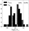 |
Fig. 1 Distribution of the B and FIR luminosities for the SB galaxies of our sample. |
2.2. Search strategy
To search SNe in the selected SB sample we used the HAWK-I instrument installed at the ESO VLT telescope at Cerro Paranal (Chile). HAWK-I is an NIR (0.85–2.5 μm) wide-field imager with a mosaic of four Hawaii-2RG detectors. The total field of view is 7.5′ × 7.5′ with a scale of 0.106″ /pix. Even in poor seeing conditions (>1.5 arcsec), the instrument allows S/N ~ 10 for a K = 20 mag star with a 15 min exposure.
The infrared light curves of SNe evolve relatively slowly, remaining within one or two magnitudes from maximum for two or three months (Mattila & Meikle 2001) and therefore an IR SN search does not require frequent monitoring. We planned for an average of three visits per galaxy per semester, for a total of 80 to 100 visits. The monitoring campaign was scheduled in service mode and we did not set tight constraints for the sky conditions. This and the relatively short duration of the observing blocks made the program well suited as filler. We notice that we had no influence on the actual scheduling of the observations that had to follow the rules of the ESO service-mode scheduler.
Eventually, the fraction of useful observing time was 100% of the allocated time in the first season, and 70% in the second and third semesters. The log of the observations is reported in Table 2 where for each galaxy we list the epoch of observations (MJD), the seeing (FWHM in arcsec), and the minimum and maximum magnitude limits for SN detection across the image (cf. Sect. 2.5). In total, we obtained 210 K-band exposures (exposure time 15 min), with an average of about three visits per galaxy per semester. Because of the time loss, three galaxies were not monitored in the last two seasons.
It turned out that the average image quality was quite good: for ~90% of the exposures, the seeing was less than 1.0″, with an average FWHM across the whole program of 0.6″.
Log of the observations.
2.3. Data reduction and analysis
For data reduction and mining of the HAWK-I mosaic images, we developed a custom pipeline that integrates different, publicly available recipes and tools in a Python environment.
The pipeline consists of four sections:
-
1.
prereduction, astrometric calibration, and production of thestacked mosaic image. For these steps we used the ESO HAWK-Ipipeline recipes in EsoRex, the ESO Recipe ExecutionTool2;
-
2.
subtraction of images taken at different epochs using ISIS (Alard 2000) for the PSF matching;
-
3.
search for transient candidates in the difference image using Sextractor (Bertin & Arnouts 1996). The candidates were ranked based on their Sextractor-measured parameters and submitted to the operator for visual inspection and validation;
-
4.
estimate of the detection efficiency through artificial star experiments performed for each of the search images (details in Sect. 2.5).
The raw images were retrieved from the ESO archive as soon as they became available, and immediately reduced to allow for activation of follow-up spectroscopy of transient candidates.
For the prereduction, we followed the reduction cascade described in the HAWK-I pipeline manual3 including dark subtraction, flat-field and illumination corrections, background subtraction, distortion correction, astrometric offset refinement, combination of the different exposures, and stitch of the four detectors in a single mosaic image. Actually, it turned out that the ESO pipeline recipes for background subtraction and offset refinement do not provide satisfactory results for our images. The main reason is the extended size of our sources and the consequent large dithering we had adopted. To address this issue we implemented custom recipes for the two aforementioned reduction steps.
The most critical step in the data reduction is image subtraction, in particular in the proximity of the nuclear regions of the galaxies. First of all we need to choose a proper reference image, usually the image with the best seeing obtained at least three month before (or in some case after) the image to be searched. We also need to choose the proper parameters for the image difference procedure (see Melinder et al. 2012 for an extensive discussion). An additional problem arises because in the distributed version of ISIS, the program automatically selects the reference sources for computating the convolution kernel. Owing to the small number of sources in our extragalactic fields, the reference source list in general includes the bright galaxy nucleus, which, being very bright, has a significant weight in the determination of the kernel. This may cause some problems, because if at one epoch an SN occurs very close to the galaxy nucleus, it can be included in the convolution kernel and effectively cancelled in the difference image. We therefore modified the ISIS selection procedure to allow for excluding specific sources, in particular the galaxy nuclei, from the reference list.
Despite efforts in many cases the difference image shows significant spurious residuals that correspond to the galaxy nuclear regions. The problem is most severe in case of images with poor seeing (FWHM > 1″) and/or reduced transparency. This is illustrated in Fig. 2 where we show two examples of image difference, one for a search image with poor seeing (FWHM = 1.5″, left panel) and the other for a case with excellent seeing (FWHM = 0.4″). In both cases, the reference image was the same and had excellent seeing (FWHM = 0.4″).
False detections due to residuals of the image subtraction were largely removed by the requirement that the candidate had to be visible at least in two consecutive epochs.
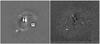 |
Fig. 2 Left panel: example of poor subtraction of images of NGC 7130 with large seeing differences (FWHM = 1.5″, with FWHM = 0.4″′ for the reference). Right panel: optimal subtraction for two images with similar good seeing (FWHM = 0.4″). In both panels the source in the lower left quadrant is SN 2010bt (cf. Fig. 3). The FOV in both panels is about 2′ × 2′. |
2.4. Supernova discoveries and characterization
During our monitoring campaign six transients were detected in at least two consecutive epochs separated by at least one month (finding charts are in Fig. 3). Four of them were spectroscopically confirmed as SNe (three SN-CC and one SN Ia), and we argue in the following that the other two transients, labeled as probable SN (PSN), are also likely SN CC (Table 3). SNe 2010bt and 2010gp were discovered and announced before our detection by optical searches but have been independently rediscovered by us.
The objects are listed in Table 3 along with the host galaxy name, distance modulus (computed from the galactocentric redshift and the adopted cosmology), SN coordinates, offsets from the galaxy nucleus, and projected linear distances from the galaxy nucleus.
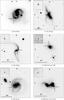 |
Fig. 3 K-band finding charts for the SNe of our list. The inserts show the transients as they appear in the difference image. |
Information for the detected SNe.
For all transients, K-band magnitudes were measured through aperture photometry on the difference images and calibrated with respect to 2MASS stars in the field. Upper limits measured on prediscovery images were also estimated. For all transients, but PSN2010 in IC 4687, we obtained some follow-up imaging in the optical or near-infrared domains. These observations were reduced using standard procedures in IRAF. When a reference image was not available, the SN magnitude was measured using the PSF fitting technique. Optical band magnitudes were calibrated with respect to Landolt’s standard fields. Our photometry for the six transients is reported in Table 4. For the two transients with no spectroscopic confirmation, the photometry is used to assess their nature.
Transient photometry.
Spectroscopic observations were obtained for four candidates: epoch, spectral range, and instruments are reported in Table 5. Data were reduced using standard procedure in IRAF but for the X-shooter spectra that were reduced using version 1.0.0 of the ESO X-shooter pipeline (Goldoni et al. 2006) with the calibration frames (biases, darks, arc lamps, and flat fields) taken during daytime. The extracted spectra, after wavelength and flux calibration, were compared with a library of template spectra using the GELATO SN spectra comparison tool4 (Harutyunyan et al. 2008). The best fit template SN, the SN type, and phase are reported in Table 5. Spectroscopic classification for PSN2010 in IC 4687 was attempted, but the observed spectrum turned out to be too noisy for a safe classification. The table includes the result of the spectroscopic observations of SN 2010gp from Folatelli et al. (2010).
Log of spectroscopic observations.
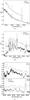 |
Fig. 4 Spectra of SN 2010bt, 2010hp, and 2011ee are shown along with the best-fitting templates. a) The spectrum of 2010bt, dereddened by AB = 1.7 mag (see text) is compared with that of the type IIn SN 1996L. b) The spectrum of 2010hp, dereddened by AB = 0,5 mag (see text) is compared with that of the type IIP SN 1999em. c) The spectrum of 2011ee is compared to that of the SN Ic 2007gr at the maximum (top panel) and 60 days after the maximum. |
We have used the available photometry and spectroscopy to put some constraints on the amount of extinction suffered by the SNe. Hereafter, we describe the sparse information available for each transient in some details.
-
SN
2010bt
was discovered on 2010 April 17.10 UT by Monard (2010). A spectrum taken on April 18.39 UT (Turatto et al. 2010) shows strong resemblance to several type-IIn SNe, in particular SN 1996L (Benetti et al. 1999) shortly after explosion (Fig. 4). A broad Hα component is present, indicating an expansion velocity of about 3500 km s-1 (half width at zero intensity). SN 2010bt was independently rediscovered by us on May 25 and was observed at other two epochs. The object was not visible on a HAWK-I image taken in 2009 July 26 (limit K = 19.0 mag). While the analysis of the light curve and spectral evolution of this SN will be presented elsewhere Elias-Rosa et al. (in prep.), a preliminary analysis shows that to match the color of SN 2010bt to that of the type IIn SN 1998S requires a significant amount of extinction (AB = 1.7 ± 0.5 mag). This extinction improves also the matching of the spectra of SN 2010bt to SN 1996L.
-
SN
2010gp
was discovered on 2010 July 14.10 UT by Maza et al. (2010) with the 0.41-m PROMPT1 telescope located at Cerro Tololo. Folatelli et al. (2010) reported the spectroscopic classification as a type-Ia SN around maximum light with high expansion velocity of the ejecta. SN 2010gp was rediscovered independently by us on July 21 and was observed at other two epochs. The object was not visible on a HAWK-I image taken on 2010 May 26 (limit K = 18.5 mag). The available colors compared to that of standard SN Ia suggest a small reddening inside the host galaxy, AB = 0.2 mag.
-
SN
2010hp
was discovered on a HAWK-I image taken on 2010 July 21.3 UT (Miluzio & Cappellaro 2010). The object was not detected on 2009 Aug. 25 (limit K = 19.0 mag). Based on a spectrum taken on 2010 Sept. 8, the SN was classified as a type II event more than 30 days past maximum light (Marion et al. 2010). We obtained a follow-up spectrum on 2010 Sept. 15 with EFOSC2 at the NTT showing the typical features of type II SN: that is, H Balmer lines, NaI D doublet, and the NIR CaII emission triplet along with a number of FeII lines in the blue region. The GELATO spectral comparison tool found a best match with the type IIP SN 1999em (Elmhamdi et al. 2003) at about +60 days, adopting a reddening of about AB = 0.5 mag (Fig. 4). This is fully consistent with the color curve comparison between the two SNe.
-
SN
2011ee
was discovered on 2011 June 27.3 UT (Miluzio et al. 2011). The object was not detected on a K-band image taken on 2010 September 7 (K > 19.0 mag). An optical spectrum was obtained with X-shooter at the VLT on 2011 July 17.3 UT showing that the transient is a type Ic SN. The GELATO code finds a best match with SN 2007gr (Hunter et al. 2009) at maximum (Fig. 4). Because the classification of type Ic SNe near maximum is sometimes ambiguous we obtained a follow-up spectrum about two months later (2011 Sept. 20) using OSIRIS at the GTC. Again the spectrum is very similar to SN 2007gr at a corresponding phase (Fig. 4 bottom panel). The color comparison and the spectral match are consistent with a negligible host galaxy extinction.
-
was discovered on 2010 May 21.3 UT in the northern component of a galaxy triplet that include IC 4686 and, 1 arcmin to the south of IC 4687, IC 4689. IC 4687 has a chaotic structure formed by stars, gas, dust, and a large curly tail. The transient was not detected on a K-band image taken on 2009 Aug. 8.1 (K > 19.0 mag). We obtained an optical/infrared spectrum with X-shooter at VLT on 2010 June 5. However, because of its very low S/N, we could not derive a convincing classification, therefore we had to rely on the K-band photometry. Comparing the K band absolute light curve of PSN2010 (AB(host) = 0) with template light curves of different SN types we found a good match with SN 2005cs, a prototype of underluminous type IIP SN (Pastorello et al. 2009), assuming that the detection of PSN2010 was two months after the explosion. However, lacking color measurements, we could not constrain the extinction, and indeed assuming a high extinction AB ~ 8 mag, we found an alternative good match with the light curve of SN 1999em (Fig. 5). Intermediate values may also be adopted by fitting other SN II.
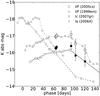
Fig. 5 K band absolute light curve of the PSN2010 (black dots), compared with those of template SNe. The empty circles show the same data but assume an extinction AB = 8 mag.
-
was discovered on 2011 July 21.4 UT in the western component of a galaxy pair. The object was not detected on a K-band image taken on 2010 Sept. 5 (K > 19.0 mag). Unfortunately, due to bad weather in the scheduled nights, we could not obtain a spectroscopic observation of the transients. We had to rely on three epochs of photometry, in K complemented by two epochs in the optical R and I bands. A simultaneous comparison of the absolute observed luminosity with template SNe gives a best fit with the SN Ic 2007gr one month after maximum (Fig. 6). Assuming this classification, from the colors we can constrain the extinction to be AB = 0.5 ± 0.5 mag. However, we have to admit that, within the errors, the photometry of PSN2011 also can be consistent with a type IIP at about three months after explosion.
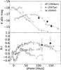
Fig. 6 K and R − I colors of PSN 2011, compared with those of template SNe. For this plot we adopted AB = 0.5 mag, which improves the fit of the R band photometry (ΔR = 0.3 mag).
2.5. Search detection limit
To derive the SN rate from the number of detected events it is crucial to obtain an accurate estimate of the magnitude detection limit for each of the search images and for different locations in the images. As shown in Fig. 2, the detection efficiency is influenced by the sky conditions at the time of observations (namely seeing and transparency) and by the transient position inside the host galaxy.
The magnitude limit for SN detection has been estimated through artificial star experiments. The procedure we adopted was the following:
-
1.
fake SNe of different magnitudes are simulated with the PSFderived from isolated field stars;
-
2.
the image is segmented into a number of intensity contour levels. We took denser contours in the nuclear regions because the magnitude limit changes rapidly with background intensity;
-
3.
one fake SN of specific magnitude is randomly placed inside a chosen intensity contour;
-
4.
the image with the fake SN is processed through the image difference and transient detection pipeline;
-
5.
if the fake SN results in a detected transient, the experiment is repeated with a fainter artificial star until we have a null detection. The fainter magnitude for which the fake SN is detected defines the magnitude limit for the given background intensity level;
-
6.
Steps 2 to 5 were repeated for each contour level three times to enhance the statistical significance of the results. The average value for each contour level has been adopted as the magnitude discovery limit for the given background intensity.
To illustrate the results, a plot of the magnitude limit versus background counts for four observations of the galaxy NGC 7130 is shown in Fig. 7. Each epoch is labeled with the image seeing, while the errorbar shows the range of limiting magnitudes for the three experiments. The top x-axis shows the linear distance in Kpc from the galaxy center.
It can be seen that, as expected, the magnitude limit is lower in the nuclear regions, which for a typical galaxy, correspond to 1.5–2.0 kpc. Epochs with different seeing have similar magnitude limits in the galaxy outskirts (typically K ~ 19 mag), while in the nuclear region when seeing is poorer the magnitude limit is brighter (in the worst case even 5–6 mag brighter than in the galaxy outskirts).
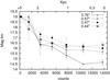 |
Fig. 7 Magnitude limit vs. background intensity for four different observations of NGC 7130. The points are labeled with the respective image seeing. Errorbars show the range of the magnitude limits from the three different experiments. |
3. SN search simulation
To evaluate the significance of the detected events we elaborated a simulation tool that returns the number and properties of expected events based on specific features of our SN search, including a number of parameters describing our current knowledge of SBs and SN properties. The tool uses a MonteCarlo approach that simulates the stochastic nature of SN explosions. By collecting several MonteCarlo experiments with the same input parameters, we can test whether the observed events are within the expected distribution. On the other hand, by varying some of the input parameters, we can test the influence of specific assumptions.
3.1. The simulation tool
Our MonteCarlo (MC) simulation tool was built in a Python environment and makes use of standard values taken from the literature for the different inputs. For those that are more controversial, we give references with some discussion. The basic ingredients of the simulation are:
-
relevant data for the selected SBs, namely: redshift, galacticextinction, infrared fluxes from IRAS catalogs at 25, 60, and100μ, B magnitude corrected for internal extinction5, Hubble morphological type. These data were retrieved from NED;
-
information describing the SN properties for each of the SN types considered here: SNe Ia and core collapse events, including SNe IIP, IIL, IIn, and Ib/c. K-band template light curves were constructed starting from B template light curves (Cappellaro et al. 1997) and B − Kk-corrections for the given galaxy redshift (Botticella et al. 2008). We note that the results of this procedure agree closely with the K template light curves of Mattila & Meikle (2001). For the SN luminosity functions we adopted those of Li et al. (2011b) as reference, but we also tested for the possible presence of a significant population of faint core collapse, which may be suggested by the analysis of very nearby SNe (Horiuchi et al. 2011). From the LOSS project we also adopted the relative rates for the different SN types (Li et al. 2011a);
-
details of the search campaign: log of observations, magnitude detection limit for each observation as a function of the host galaxy background intensity;
-
the number of SNe expected from a given star formation episode. For core collapse SNe, this is determined only by the adopted mass range of the progenitors and IMF slope. In fact, for our purposes, we can neglect the very short time delay from CC progenitor formation to explosion. For type Ia SNe, we need to consider the realization factor, which is the fraction of events in the proper mass range, which occurs in suitable close binary systems and the delay-time distribution (Sect. 3.1.2);
-
the depth and distribution of the extinction by dust inside the parent galaxies (cf. Sect. 3.1.3);
-
the star formation spatial distribution in the parent galaxies (cf. Sect. 3.1.4).
Hereafter, we discuss our assumptions about the parameters of the simulation.
3.1.1. From IRAS measurements to star formation rate
The SFR in SBs can be estimated on the basis of the galaxy total infrared luminosity (LTIR) under the assumption that dust reradiates a major fraction of the UV luminosity and after calibration with stellar synthesis models. The TIR luminosity can, in turn, be estimated from FIR flux measurements.
Helou et al. (1988) provided a prescription for
deriving the FIR emission from IRAS measurements: ![Mathematical equation: \begin{eqnarray*} { \rm FIR} = 1.26 \times 10^{-14}\, [2.58 \, f_\nu(60~\mu {\rm m}) + f_\nu(100~\rm \mu m)] \end{eqnarray*}](/articles/aa/full_html/2013/06/aa21192-13/aa21192-13-eq113.png) where
FIR is in W m-2 and fν are in
Jansky. FIR fluxes are converted into TIR fluxes by using the relation of Dale et al.
(2001)
where
FIR is in W m-2 and fν are in
Jansky. FIR fluxes are converted into TIR fluxes by using the relation of Dale et al.
(2001)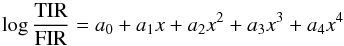 where
where
 and [a(z = 0)] ≃ [0.2378, − 0.0282, 0.7281, 0.6208,
0.9118].
and [a(z = 0)] ≃ [0.2378, − 0.0282, 0.7281, 0.6208,
0.9118].
The TIR fluxes are converted in luminosities using the adopted distances:
 Finally,
the relation between the SFR (ψ) and LTIR
was derived by Kennicutt (1998) from SB galaxy
spectral synthesis model adopting 10–100 Myr continuous bursts and a Salpeter IMF as
Finally,
the relation between the SFR (ψ) and LTIR
was derived by Kennicutt (1998) from SB galaxy
spectral synthesis model adopting 10–100 Myr continuous bursts and a Salpeter IMF as
![Mathematical equation: \begin{eqnarray*} \frac{\psi}{[M_\odot\, {\rm yr}^{-1}]} = \frac{L_{\rm TIR}}{2.2 \times 10^{43} ~~ [{\rm erg}\,{\rm s}^{-1}]} = \frac{L_{\rm TIR}}{5.8 \times 10^9 ~~ [L_\odot]}\cdot \end{eqnarray*}](/articles/aa/full_html/2013/06/aa21192-13/aa21192-13-eq122.png)
3.1.2. SNR and SFR
In general, the rate of SNe expected at a specific time,
ṅSN(t), for a stellar population depends
on the star formation history, the number of SNe per unit mass from one stellar
generation (labeled as SN productivity), and the distribution of delay time from star
formation to explosion for the specific SN type. Following the notation of Greggio (2005, 2010),  (1)where
ψ(t) is the SFR, fSN is
the distribution of the delay times τ and
kSN is the SN productivity. The equation shows that at a
fixed epoch t since the beginning of star formation, the rate of SNe is
obtained by adding the contribution of all past stellar generations, each of them
weighted with the SFR at the appropriate time.
(1)where
ψ(t) is the SFR, fSN is
the distribution of the delay times τ and
kSN is the SN productivity. The equation shows that at a
fixed epoch t since the beginning of star formation, the rate of SNe is
obtained by adding the contribution of all past stellar generations, each of them
weighted with the SFR at the appropriate time.
Core collapse SNe
For core collapse SNe the delay time from star formation to explosion (2.5 Myr for 120
M⊙ stars up to 40 Myr for 8 M⊙
stars) is shorter than the typical SB duration (200–400 Myr, McQuinn et al. 2009). Assuming that the SFR in the SB was constant
during the past 40 Myr, the expected CC SN rate, ṅCC, is
proportional to the current SFR:  The
SN productivity kCC is derived by integrating the IMF,
φ(m), and assuming a CC progenitor mass
(MCC) range:
The
SN productivity kCC is derived by integrating the IMF,
φ(m), and assuming a CC progenitor mass
(MCC) range:  where
where
 and
and
 are respectively
the lower and upper mass limits for SN CC progenitors, and
ML and MU are the lower and
upper stellar mass limit. To be consistent with the Kennicutt SFR calibration we adopted
a Salpeter IMF, that is,
are respectively
the lower and upper mass limits for SN CC progenitors, and
ML and MU are the lower and
upper stellar mass limit. To be consistent with the Kennicutt SFR calibration we adopted
a Salpeter IMF, that is,  Assuming
8 < MCC < 50 M⊙
for the CC progenitor mass range,
kCC = 0.007 M-1. This number changes
significantly if we adopt a different IMF, e.g. kCC = 0.011
for a Kroupa IMF or kCC = 0.039 for an extreme Starburst IMF
(Dwek et al. 2011). We soon note, however that,
because the IMF also enters into the conversion from LTIR to
ψ, the expected rate of SN events is almost independent of the
selected IMF (cf. Sect. 4.1), provided the choice
is consistent.
Assuming
8 < MCC < 50 M⊙
for the CC progenitor mass range,
kCC = 0.007 M-1. This number changes
significantly if we adopt a different IMF, e.g. kCC = 0.011
for a Kroupa IMF or kCC = 0.039 for an extreme Starburst IMF
(Dwek et al. 2011). We soon note, however that,
because the IMF also enters into the conversion from LTIR to
ψ, the expected rate of SN events is almost independent of the
selected IMF (cf. Sect. 4.1), provided the choice
is consistent.
More important is the assumption on the mass range for CC progenitors, which is not
well constrained. Actually, while changing the upper limit of the progenitor mass from
40 to 100 M⊙ makes a modest 10% increase in the CC SN
productivity, the lower mass limit is crucial, with kCC
decreasing by 30% if we adopted  instead of the
favored value of 8 M⊙ (Smartt 2009).
instead of the
favored value of 8 M⊙ (Smartt 2009).
SN Ia
Estimating the expected rate of SN Ia is complicated because the delay time distribution fIa, while still uncertain, certainly ranges from short to a very long time. In particular, it has been suggested that SN Ia can be divided into two classes, one with a short delay time whose rate scales with the current SFR (also called prompt), and a second with a long delay time (tardy), whose rate scales with the average of the SFR during the entire galactic evolution (Scannapieco & Bildsten 2005; Mannucci et al. 2006). While stellar evolution arguments (Greggio 2010, 2005; Greggio & Renzini 1983) and more recent data (Maoz et al. 2012; Totani et al. 2008) suggest a continuous distribution of the delay time instead of two distinct classes, the schematization is still a fair approximation that helps in simplifying the problem of predicting the expected SN Ia rate in SBs.
In general, for a galaxy of the local Universe, ~ 13 Gyr after the beginning
of SFR, we can identify the contribution of the two components as follows (Greggio 2010): 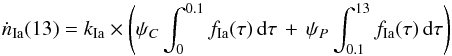 (2)where
ψC and
ψP are the average SFR over,
respectively, the last 0.1 Gyr (current SFR) and from 0.1 to 13 Gyr ago (past SFR). The
SN productivity kIa is the product of the number of stars
per unit mass in the adopted progenitor mass range (0.021 for a Salpeter IMF and a mass
range
3 M⊙ < M < 8 M⊙)
and the realization fraction, the actual fraction of systems which make a successful
explosion (~ 5% according to the most recent estimate) (Maoz & Mannucci 2012). We assume that SF history in SBs can
be described schematically with two components: a constant SFR during the galaxy
evolution that created the galaxy stellar mass, and an ongoing episode of intense SFR
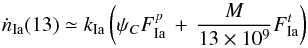
that is the source of the strong TIR emission. Neglecting the contribution of the
ongoing SB to the galaxy stellar mass, we can approximate
ψP ≃ M/13 × 109
and write Eq. (2) as
(2)where
ψC and
ψP are the average SFR over,
respectively, the last 0.1 Gyr (current SFR) and from 0.1 to 13 Gyr ago (past SFR). The
SN productivity kIa is the product of the number of stars
per unit mass in the adopted progenitor mass range (0.021 for a Salpeter IMF and a mass
range
3 M⊙ < M < 8 M⊙)
and the realization fraction, the actual fraction of systems which make a successful
explosion (~ 5% according to the most recent estimate) (Maoz & Mannucci 2012). We assume that SF history in SBs can
be described schematically with two components: a constant SFR during the galaxy
evolution that created the galaxy stellar mass, and an ongoing episode of intense SFR
that is the source of the strong TIR emission. Neglecting the contribution of the
ongoing SB to the galaxy stellar mass, we can approximate
ψP ≃ M/13 × 109
and write Eq. (2) as
 where
where
 and
and
 are the relative
fraction of prompt and tardy events derived by integrating the delay time distribution
in the relevant time range. In our approximation,
ψC can be derived from the observed
LTIR and the galaxy mass from the K
magnitude and B − K colors (cf. Mannucci et al. 2005).
are the relative
fraction of prompt and tardy events derived by integrating the delay time distribution
in the relevant time range. In our approximation,
ψC can be derived from the observed
LTIR and the galaxy mass from the K
magnitude and B − K colors (cf. Mannucci et al. 2005).
The relative contribution of the two SN Ia components has been a very debated issue in
the past few years, ranging from  (Mannucci et al. 2006) to
 from
standard stellar evolution scenarios (Greggio
2010). In our simulation we adopted an intermediate value,
from
standard stellar evolution scenarios (Greggio
2010). In our simulation we adopted an intermediate value,
 as
reference.
as
reference.
3.1.3. Extinction
Dust extinction in SBs is very high, especially in the nuclear regions. For instance, Shioya et al. (2001) find that fitting the spectral energy distribution of the nuclear region of Arp 220 requires a visual extinction AV > 30 mag. Actually, according to Engel et al. (2011), “over most of the disk the near-infrared obscuration is moderate, but increases dramatically in the central tens of parsecs of each nucleus”. Similar high extinction, AV ~ 20, was found for the SB region of Zw 096 (Inami et al. 2010).
Morphological classification, FIR colors, and compactness classification for the SBs of our sample.
As a first-order approximation, for our simulation we assumed that the extinction has the same distribution of the SF (see next section) with a maximum value AV = 30 mag corresponding to the SFR peak and scaled linearly in the other regions. While this is a crude approximation, it turns out that the actual choice of extinction correction has little impact on our simulation. In the nuclear, high-extinction regions, the SN detection is limited by the reduced performance of the image subtraction algorithm in these high surface-brightness regions. At the same time, our IR search is largely insensitive to variation in the (moderate) extinction of the outer galaxy regions.
For the wavelength dependence of extinction, we adopted the Calzetti’s law with RV = 4.05 ± 0.8 (Calzetti et al. 2000).
3.1.4. Star formation distribution
The spatial distribution of the SFR is a key ingredient of the simulation. This is because we expect that SNe occur more frequently in the high SF regions where, on the other hand, our detection efficiency is lower. In principle, the FIR emission that is used to estimate the SFR would also be a good tracer of its spatial distribution. However, it turned out that the available MIR imaging for the galaxies of our sample (mainly obtained with the Spitzer observatory) does not have enough spatial resolution for mapping the compact SB structures.
Selected K-band images from our survey can have excellent resolution, but as is well-known, the near IR emission traces the old star population better, which is the galaxy mass distribution more than the SFR distribution. Therefore for an estimate of the SFR concentration, we are forced to an indirect, statistical approach.
Our starting point is the SB classification by Hattori et al. (2004), who derived a correlation between the global SBs properties, such as FIR colors, and the compactness of the SF regions. These range from very compact (≤100 pc) nuclear starbursts with almost no star-forming activity in the outer regions (type 1), to extended starbursts with relatively faint nuclei (type 4), with types 2 and 3 as intermediate cases. In addition, they find a trend for galaxies with more compact SF region to show a higher star formation efficiency and hotter far-infrared color. They also find that the compactness of SF regions is weakly correlated with the galaxy morphology, with disturbed objects primarly showing more concentrated SF. On the other hand, an appreciable fraction (~ 50%) of their galaxy sample was dominated by extended starbursts (type 4). The significant variations in the degree of concentration of the SB SF regions has been recently confirmed by McQuinn et al. (2012).
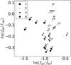 |
Fig. 8 FIR color of the SBs of our sample. The different symbols identify the compactness class (Hattori et al. 2004), while the label shows the morphological type. |
Input parameters for the reference simulation.
For the reference simulation we used the input parameters summarized in Table 7. In the next section we compare the prediction of the simulation with the current SN discoveries. In an attempt to characterize the SF spatial distribution for the SBs of our sample, we derived estimates of their morphological class and FIR colors. In particular, following Hattori et al. (2004), SBs with strong tidal features and a single nucleus were classified as “mergers” (M), galaxy pairs with an overlapping disk or a connecting bridge were classified as “close pairs” (CP) if the projected separation is <20 Kpc and galaxies that have a nearby (<100 Kpc) companion at the same redshift were classified as “pairs” (P). The remaining objects were classified as “single” (S). The classification of the SBs of our sample is listed in Table 6 along with the galaxy FIR colors, log f60/f100, log f25/f60.
We attributed to each galaxy a compactness class on the basis of its correlation with the FIR colors as shown in Fig. 4 of Hattori et al. (2004), which for the object of our sample corresponds to our Fig. 8. As can be seen, we also confirmed their claim of a (weak) relation of FIR color and, as a consequence, compactness class with SB morphology.
The next step is based on Soifer et al. (2000, 2001). For several SBs galaxies they plotted the MIR and NIR emission curve of growth finding that, in general, the MIR emission is more concentrated, while only for a few galaxies do the MIR and NIR curves of growth show a similar trend. Actually we found that, to a first-order approximation, the MIR emission profile of a given galaxy can be matched by NIR profile powered to an exponent α, which ranges between 1, when the two profiles are similar, to 2, when the MIR emission is strongly concentrated. When we classified the same galaxies with the compactness criteria of Hattori et al. (2004), we find that (as expected) the galaxies with compact SF regions (types 1–2) are characterized by more concentrated MIR emission (α = 2.0–1.5, respectively), while galaxies with extended SF region (types 3–4) have similar MIR vs. NIR profiles (α = 1.25–1.0, respectively). As a reference, we notice that in the typical case of NGC 6240, assuming α = 1 corresponds to locate 50% of the SFR within 1.5 Kpc, whereas for α = 2 the same SFR fraction is enclosed within 500 pc.
As a result of this discussion we estimate the SF distribution based on the observed LK, and adopt a power index α appropriate to the compactness class of the given SB galaxy (Table 7).
3.1.5. Flow chart of the simulation
Having defined all the ingredients of the simulation, we can now describe how this proceeds. The simulation flowchart can be summarized as follows:
-
1.
For each galaxy of the sample, based on the estimated total SFRand adopted progenitor scenarios, we compute the expectednumber of SNe per year.
-
2.
A time interval is chosen so that 100 SNe are expected to explode in the given galaxy in that period. The time interval ends with the last observations of the galaxy. Given the expected SN rates, it is much longer for all galaxies than the duration of our monitoring campaign. The reason for simulating 100 events is to avoid having to deal with fractional SN numbers for the different subtypes. We assign to each event a random epoch of explosion chosen within the defined time interval.
-
3.
Each SN is assigned to a random explosion site inside the parent galaxy according to the SFR spatial distribution.
-
4.
A peak magnitude is also assigned to each SN, with a random value derived from the adopted SN luminosity function for the specific subtype. We also associate an extinction value to the event that is randomly extracted from a Gaussian distribution whose mean value depends on the position of the SN, and σ = 1/3 of the mean value.
-
5.
The apparent magnitude is thereafter calculated at the epochs of available observations, knowing the galaxy distance modulus and SN epoch of explosion. This is compared with the search’s magnitude detection limit for the given position, and when brighter, the SN is added to the simulated discovery list.
The process, iterated for all the galaxies of the sample, defines a single simulation run. Outcomes of the simulation are the expected number of SN discoveries, their types, magnitudes, extinctions, and positions inside the host galaxies. To explore the distribution of the outcomes from the random process, a complete experiment is made by collecting a minimum of a hundred single simulation runs.
4. Comparison between observed and expected SN discoveries
As we outlined above, from many of MonteCarlo simulation runs we obtain the distribution of the expected SN discoveries. This is shown in Fig. 9, where each bin of the histogram is the predicted probability of observing the specific number of SN discoveries, whereas the dashed line marks the number of actual SNe discovered and the shaded area shows its 1-σ Poissonian uncertainty range.
We found that with the adopted simulation scenario and input parameters, we should have expected, on average, to discover 5.3 ± 2.3 SNe. In 68% of the experiments (1-σ) the expected number is in the range 4–8, which is in excellent agreement with the observed number of six events. The prediction of the simulation is that almost all SNe are CC (5.1 SN CC vs. 0.2 SN Ia), though in 10% of the experiments at least one type Ia is found (that is what we have from the real SN search).
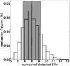 |
Fig. 9 Histogram of the number of expected SNe from our MonteCarlo experiments. The dashed vertical line indicates the number of observed events and the gray area its 1σ-Poissonian uncertainty. |
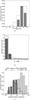 |
Fig. 10 SN property comparison. a) Expected (line-only) and observed (gray) K magnitude distribution at the discovery. b) Expected (line-only) and observed (gray) extinction distribution. In light gray we indicate the allowed range for the extinction of PSN2010 (see text). c) Radial distribution of expected (line-only) and detected (dark grey) SNe. For regular galaxies the surface brightness decreases monotonically with radial distance. The upper axis shows this correspondence for one of the galaxy of our sample. In light gray we show the distribution of injected artificial SNe (see text). |
The distributions of some of the expected and observed SN properties are compared in Fig. 10. For the simulation, we show the distribution across the different experiments (line-only histogram) while the grey shaded histogram represents the actual observations.
The top panel in Fig. 10 shows the distribution of the apparent magnitudes at the discovery. The good agreement between simulations and observations is a crucial consistency check of our estimates of the magnitude detection limit: if the discovered SNe were systematically fainter/brighter then expected, this would indicate an underestimate/overestimate of the search detection efficiency.
A comparison of the simulated vs. observed extinction distribution is shown in the middle panel of Fig. 10. For the observed distribution, the case of PSN2010 is shown for which extinction is ambiguous is shown. Again the simulation is in good agreement with the observations. This argues in favor of the consistency of the input assumptions. The fact that, in our IR search, we expect that most detected SNe have low extinction (~ 75% with AV < 1 mag) is a consequence of our assumption that the extinction is very high in the nucleus and rapidly decreases with the galaxy radius, following the same trend in the SFR. This does not mean that extinguished SN are intrinsically rare, but that they are confined to the galaxy nuclear regions where extinction is extremely high even in the IR (see next). At the same time we can exclude the presence of any significant population of SNe with intermediate extinctions: we would easily detect them in our infrared search. Mattila & Meikle (2001) find an average value of AV = 30 mag for the extinction towards the SN remnants of M82, confirming the presence of high extinction (about AV ~ 15–45 mag) in the innermost 300 pc regions. On the other hand, Kankare et al. (2008) find an host galaxy extinction of AV ~ 16 mag for the SN 2008cs, located at about 1.5 Kpc, so relatively far from the galaxy nucleus.
Finally, in the bottom panel of Fig. 10 we compare the distribution of locations inside the host galaxy for the expected vs. observed SNe. The different location are identified by the K band pixel counts: in general high counts occur in the nuclear regions, while low counts are in the outskirts. We use pixel counts instead of radial distances because the latter is difficult to be defined for galaxies with irregular morphology or double nuclei. However an indicative correspondence from pixel count to radial distance is shown at the top axis of the figure for a galaxy with regular morphology. There is a mild indication of a deficiency of observed events in regions with high pixel counts. Taken at face value this may suggest a minor overestimate of the detection magnitude limit in the nuclear regions. Given the lack of statistics we cannot raw definite conclusions and therefore will not develope this issue further.
In the same figure we also show the distribution of locations of the expected events for an ideal case where the magnitude detection limit in the nuclear regions is as deep as in the outskirts and extinction is negligible. The experiment shows that the fraction of events that remain hidden to our search in the galaxy nuclear regions due to the combined effect of reduced search efficiency, and extinction is very high, about 60% (cf. Mattila et al. 2012).
4.1. Uncertainties and effect of different assumptions
Magnitude detection limit
One of the main sources of uncertainty for the simulation is related to the estimate of the magnitude detection limit, maglim. For the reference simulation, we adopted the mean value as maglim out of three artificial star experiments conducted for several selected positions inside the host galaxy (cf. 2.5). The dispersion of measurements, which is the uncertainty on maglim, is quite large with a typical range of ~0.5 mag, but in more extreme difficult cases, it can be as large as 2 mag.
To test the propagation of this uncertainty, we performed MonteCarlo experiments by alternatively assuming the lower and higher maglim out of the three experiments. We found that the predicted number of SNe is 6.2 ± 2.5 and 4.7 ± 2.2, which are + 17% and − 11% with respect to the numbers from the reference simulation. That error is significant is why we made a significant effort to get a detailed estimate of the detection limit.
SN luminosity function
In the reference simulation we use a Gaussian distribution for the SN luminosity function (SN-LF) with a mean value and dispersion taken from Li et al. (2011b). However, based on a small sample of very nearby SNe, Horiuchi et al. (2011) claim that the faint end of the SN-LF is underestimated, and SN CC fainter than mag ≃ − 16 could make up to 50% of the distribution, to be compar with 20% of the sample of Li et al. (2011b). On the other hand, Mattila et al. (2012) argue that Horiuchi et al. (2011) overestimated the fraction of intrisically faint CCSNe since they neglect the host galaxy extinction for their SN absolute magnitudes. We performed a MonteCarlo experiment that adopt the Horiuchi’s SN-LF and found that in this case the expected number of events would be low, only 3.3 on average. This is because most faint events are expected to fall below the search detection limit. That the actual discoveries are twice this number argues against a large fraction of faint SN-CC (cf. Botticella et al. 2012).
IMF and SN CC progenitor mass range
The IMF enters both in the estimate of the number of SN progenitors and in the
calibration of TIR luminosity in terms of SFR relation. However, the expected rate of CC
SNe in our sample is virtually independent of the IMF slope. Indeed, for a given total
mass of the parent stellar population, top heavy IMFs imply both more of CC progenitors
and higher luminosity. Following Dwek et al.
(2011), the number of CC progenitors per unit mass is
kCC = 0.007,0.011, and 0.039
M⊙-1 for a Salpeter, a Kroupa, and a Starburst
IMF respectively, assuming that the progenitors range from 8 to 50
M⊙. At the same time, the total luminosity of an SB forming
stars with an SFR of 1 M⊙ yr-1 over a period of
10 Myr (i.e. a 107M⊙ stellar population) is
4.71 × 10⁹, 7.33 × 10⁹, and
2.55 × 10¹⁰L⊙ again for a Salpeter, a Kroupa, and
a Starburst IMF. The M/L ratio of such SBs is then 0.0021, 0.0014, and 0.0004 (solar
units) for the three IMFs, and the expected number of CC SNe originating from it is ≃1.5
every  for all three IMFs. Working out the numbers, it turns out that the SN CC rates from a
population with a given LTIR is almost independent of the IMF,
provided a consistent choice is made.
for all three IMFs. Working out the numbers, it turns out that the SN CC rates from a
population with a given LTIR is almost independent of the IMF,
provided a consistent choice is made.
Crucial is instead the assumption of the SN CC progenitor mass range, in particular, the lower limit. Indeed if we adopted an upper limit of 100 M⊙ instead of the reference value of 50 M⊙, the expected number of SNe would be 5.5 ± 2.1, only ~5% higher then the reference simulation. On the other hand, assuming a lower limit of 10 M⊙ (instead of 8 M⊙) results in an expected number of SNe of 3.9 ± 2.1, which is ~30% lower than the expected rate obtained in the reference case.
Extinction
For the reference case we assumed that the extinction scales with the SFR with a maximum value corresponding to the SFR peak AV = 30 mag. To test the uncertainty related to this assumption, we made two different tests. In one experiment we maintained the relation of AV with SFR but taking, alternatively, peak extinction values AV = 10 and AV = 100 mag. The experiment gave 5.5 ± 2.7 and 4.7 ± 2.3 respectively as expected number of SNe. In the second experiment we assumed that the extinction is constant through the galaxy and is AV = 3.0 mag. In this case the expected number is 5.3 ± 2.3, so identical to the value of the reference simulation.
The conclusion is that the uncertainty on the extinction does not significantly affect the simulation or, conversely, that our experiment cannot probe the extinction distribution.
Star formation distribution
The spatial distribution of SFR is an important, and the most uncertain, ingredient of the simulation. For instance, if we assume that the SFR is confined in the very inner regions, say in the inner 3–500 pc, the resulting SNe will remain inaccessible to our search. On the other hand, that the SFR is extended in some SBs has been confirmed by different studies (eg. McQuinn et al. 2012), not to mention that many of the SNe we have discovered are at significant radial distances (cf. Table 3).
As described in Sect. 3.1.4, as proxy of the SFR
distribution we use  where
α range from 1 to 2 depending on the galaxy compactness class (Table
6). To test for the uncertainties of this
assumption we performed two simulations that assume that α is either 1 or
2 for all galaxies. We obtained an expected rate of 8.8 ± 3.0 in the first case and in the
second case a value of 3.0 ± 1.7. The latter occurs because when the SFR is more
concentrated, a large number of SNe remain hidden to our search due to the low search
detection efficiency in the nuclear regions.
where
α range from 1 to 2 depending on the galaxy compactness class (Table
6). To test for the uncertainties of this
assumption we performed two simulations that assume that α is either 1 or
2 for all galaxies. We obtained an expected rate of 8.8 ± 3.0 in the first case and in the
second case a value of 3.0 ± 1.7. The latter occurs because when the SFR is more
concentrated, a large number of SNe remain hidden to our search due to the low search
detection efficiency in the nuclear regions.
The conclusion is that the uncertainty in the adopted SF distribution propagates with an error of ~ 50% on the expected SN number. We may consider that the actual good match of observations with the reference simulation argues in favor of the adopted prescription.
5. Summary and conclusions
We have presented the analysis of an infrared SN search in a sample of 30 nearby SB galaxies, conducted between 2009 and 2011, with the goal verifying the link between star formation and the SN rate. During our search we collected about 240 observations in total, discovering 6 SNe, 4 of them with spectroscopic confirmation.
To verify how this number compare with expactations we performed a detailed characterization of the SN detection efficiency, the galaxy properties (in particular SF rate and spatial distribution), and the SN properties and progenitor scenarios. We included all these ingredients in a MonteCarlo simulation tool that, after allowing for the stochastic nature of SN events, can be used to explore the distribution of the expected SN number and properties.
First of all, we may point out that by itself the number of detected SNe is proof of the high SFR in SBs. In fact if we computed the expected number of SNe in our survey based on the average SN rate per unit B luminosity or mass (Li et al. 2011a), we would predict the discovery of 0.5 events (or more precisely, 50% of the simulation predict the discovery of one event and none is expected in the other 50%). The observed number is one order of magnitude higher, which is consistent with the fact that the TIR emission of SBs is about ten times higher than for normal SF galaxies with the same B luminosity. Indeed, it is well known that the TIR luminosity is an excellent tracer for SFR, in particular in SBs.
When we adopted the SFR from LTIR as input for the MonteCarlo experiment, we found that the expected number of SNe in our search is 5.3 ± 2.3, SNe in excellent agreement with observations.
We performed a number of tests to verify the dependence of the simulation outcomes from the
input parameters. For the SN search characterization we show that an accurate estimate of
the magnitude limit for SN detection is crucial. This is why we made a considerable effort
in artificial star experiments (possibly the single most expensive task of our project). For
the galaxy characterization, the most uncertain input is the SF spatial distribution. With
some creativity, we devised a prescription that seems to work, but it is certain that this
is a place for improvements when new, high-resolution SB maps become available. Instead, we
found that our results are not sensitive to the uncertainty on the amount of extinction
because where extinction is very high (the dense SB regions) our search is limited by the
bright magnitude detection limit. SNe in these regions remain hidden to our search almost
independently of the amount of extinction. Based on our simulation we estimated that the
fraction of hidden SNe is very significant, that is, ~ 60% with an upper limit of
75%, if we account for the Poissonian uncertainties in the number of detected events.
Finally, for the SN progenitor scenarios the larger uncertainty is the lower limit of the
progenitor mass range. If we adopt a lower limit  instead of
8 M⊙ as in the reference simulation, the expected number of
SNe would be 30% lower than observed.
instead of
8 M⊙ as in the reference simulation, the expected number of
SNe would be 30% lower than observed.
Our results appear to agree with those of previous, similar searches (Mannucci et al. 2003; Cresci et al. 2007; Mattila et al. 2007a, 2012, cf. Sect. 1). In broad terms, the overall conclusion of all these studies can be expressed as follows. The number of (CC) SNe found in SBs galaxies is consistent with what is predicted from the high SFR (and the canonical mass range for the progenitors) when we recognize that a major fraction of the events remain hidden in the inaccessible SB regions. As stressed by Mattila et al. (2012), this has important consequences for the use of SN CC as a probe of the cosmic SFR, because the fraction of SBs is expected to increase with redshifts (cf. Melinder et al. 2012; Dahlen et al. 2012)
While continuing to search for SNe in SBs, in the optical, and infrared, it can certainly help to improve the still lack of statistics, one may argue at this point for a change in strategy.
In this respect a good example is the attempt to reveal some of the hidden SN CC through infrared SN searches that exploit adaptive optics at large telescopes, e.g. Gemini or VLT. The results are encouraging with the discovery of two SNe with very high extinction, namely SN 2004ip with AV between 5 and 40 mag (Mattila et al. 2007b) and SN 2008cs with AV 16 mag (Kankare et al. 2008), though we may notice that both objects were too faint for spectroscopic confirmation. Other two SNe were discovered very close to the galaxy nucleus, namely SN 2010cu at a radial distance of 180 pc and SN 2011hi at 380 pc (Kankare et al. 2012), though in these cases the low extinction suggests that the low radial distance is a projection effect. Also in these cases no spectroscopic classification was obtained. The extinction towards SN 2011hi was revised by Romero-Cañizales et al. (2012) using Gemini-N data. They demonstrate that this is most likely an SN IIP with AV of 5–7 mag. Because of the need to monitor one galaxy at a time and to access heavily subscribed large telescopes, this approach will not result in large statistical sample though even a few events may be mostly valuable for exploring the very obscured nuclear regions.
On the other hand, a new opportunity that should be explored is the piggy-back-on-wide-field extragalactic surveys of the next generation of infrared facilities, in particular EUCLID. This would allow IR SN searches to be performed for the first time on a large sample of galaxies exploring a range of SF activity and, by monitoring galaxies at different redshifts, probe the cosmic evolution.
The NASA/IPAC Extragalactic Database (NED) is operated by the Jet Propulsion Laboratory, California Institute of Technology, under contract with the National Aeronautics and Space Administration.
The galaxy internal extinction was retrieved from HyperLeda (Paturel et al. 2003).
Acknowledgments
We thank the referee, Seppo Mattila, for the careful reading and the very useful comments. We give particular thanks to Anna Feltre (ESO) for her help in estimating the possible contribution by AGNs to the FIR luminosity of the galaxies and to Barbara Lo Faro (Astronomy Department of Padova) for helpful discussions and suggestions. We acknowledge the support of the PRIN-INAF 2009 with the project “Supernovae Variety and Nucleosynthesis Yields”. E.C., L.G., S.B., A.P., and M.T. are partially supported by the PRIN-INAF 2011 with the project “Transient Universe: from ESO Large to PESSTO”. N.E.R. acknowledges financial support by the MICINN grant AYA08-1839/ESP, AYA2011-24704/ESP, and by the ESF EUROCORES Program EUROGENESIS (MINECO grants EUI2009–04170). F.B. acknowledges support from FONDECYT through Postdoctoral grant 3120227 and from the Millennium Center for Supernova Science through grant P10-064-F (funded by “Programa Bicentenario de Ciencia y Tecnologia de CONICYT” and “Programa Iniciativa Cientifica Milenio de MIDEPLAN”).
References
- Alard, C. 2000, A&AS, 144, 363 [NASA ADS] [CrossRef] [EDP Sciences] [Google Scholar]
- Bazin, G., Palanque-Delabrouille, N., Rich, J., et al. 2009, A&A, 499, 653 [NASA ADS] [CrossRef] [EDP Sciences] [Google Scholar]
- Benetti, S., Turatto, M., Cappellaro, E., Danziger, I. J., & Mazzali, P. A. 1999, MNRAS, 305, 811 [NASA ADS] [CrossRef] [Google Scholar]
- Bertin, E., & Arnouts, S. 1996, A&AS, 117, 393 [NASA ADS] [CrossRef] [EDP Sciences] [Google Scholar]
- Blanc, G., & Greggio, L. 2008, New A, 13, 606 [Google Scholar]
- Botticella, M. T., Riello, M., Cappellaro, E., et al. 2008, A&A, 479, 49 [NASA ADS] [CrossRef] [EDP Sciences] [Google Scholar]
- Botticella, M. T., Smartt, S. J., Kennicutt, R. C., et al. 2012, A&A, 537, A132 [NASA ADS] [CrossRef] [EDP Sciences] [Google Scholar]
- Bregman, J. D., Temi, P., & Rank, D. 2000, A&A, 355, 525 [NASA ADS] [Google Scholar]
- Calzetti, D., Armus, L., Bohlin, R. C., et al. 2000, ApJ, 533, 682 [NASA ADS] [CrossRef] [Google Scholar]
- Cappellaro, E., Turatto, M., Tsvetkov, D. Y., et al. 1997, A&A, 322, 431 [NASA ADS] [Google Scholar]
- Cappellaro, E., Evans, R., & Turatto, M. 1999, A&A, 351, 459 [NASA ADS] [Google Scholar]
- Cappellaro, E., Riello, M., Altavilla, G., et al. 2005, A&A, 430, 83 [NASA ADS] [CrossRef] [EDP Sciences] [Google Scholar]
- Cresci, G., Mannucci, F., Della Valle, M., & Maiolino, R. 2007, A&A, 462, 927 [NASA ADS] [CrossRef] [EDP Sciences] [Google Scholar]
- Dahlen, T., Strolger, L.-G., Riess, A. G., et al. 2004, ApJ, 613, 189 [NASA ADS] [CrossRef] [Google Scholar]
- Dahlen, T., Strolger, L.-G., Riess, A. G., et al. 2012, ApJ, 757, 70 [NASA ADS] [CrossRef] [Google Scholar]
- Dale, D. A., Helou, G., Contursi, A., Silbermann, N. A., & Kolhatkar, S. 2001, ApJ, 549, 215 [NASA ADS] [CrossRef] [Google Scholar]
- Dwek, E., Staguhn, J. G., Arendt, R. G., et al. 2011, ApJ, 738, 36 [NASA ADS] [CrossRef] [Google Scholar]
- Elmhamdi, A., Danziger, I. J., Chugai, N., et al. 2003, MNRAS, 338, 939 [NASA ADS] [CrossRef] [Google Scholar]
- Engel, H., Davies, R. I., Genzel, R., et al. 2011, ApJ, 729, 58 [NASA ADS] [CrossRef] [Google Scholar]
- Folatelli, G., Gutierrez, C., & Pignata, G. 2010, Central Bureau Electronic Telegrams, 2390, 1 [NASA ADS] [Google Scholar]
- Gallagher, III, J. S. 1993, in Massive Stars: Their Lives in the Interstellar Medium, eds. J. P. Cassinelli, & E. B. Churchwell, ASP Conf. Ser., 35, 463 [Google Scholar]
- Goldoni, P., Royer, F., François, P., et al. 2006, in SPIE Conf. Ser., 6269 [Google Scholar]
- Graur, O., Poznanski, D., Maoz, D., et al. 2011, MNRAS, 417, 916 [NASA ADS] [CrossRef] [Google Scholar]
- Greggio, L. 2005, A&A, 441, 1055 [NASA ADS] [CrossRef] [EDP Sciences] [Google Scholar]
- Greggio, L. 2010, MNRAS, 406, 22 [NASA ADS] [CrossRef] [Google Scholar]
- Greggio, L., & Renzini, A. 1983, A&A, 118, 217 [NASA ADS] [Google Scholar]
- Grossan, B., Spillar, E., Tripp, R., et al. 1999, AJ, 118, 705 [Google Scholar]
- Harutyunyan, A. H., Pfahler, P., Pastorello, A., et al. 2008, A&A, 488, 383 [NASA ADS] [CrossRef] [EDP Sciences] [Google Scholar]
- Hattori, T., Yoshida, M., Ohtani, H., et al. 2004, AJ, 127, 736 [NASA ADS] [CrossRef] [Google Scholar]
- Helou, G., Khan, I. R., Malek, L., & Boehmer, L. 1988, ApJS, 68, 151 [NASA ADS] [CrossRef] [Google Scholar]
- Hopkins, A. M., & Beacom, J. F. 2006, ApJ, 651, 142 [NASA ADS] [CrossRef] [MathSciNet] [Google Scholar]
- Horiuchi, S., Beacom, J. F., Kochanek, C. S., et al. 2011, ApJ, 738, 154 [NASA ADS] [CrossRef] [Google Scholar]
- Hunter, D. J., Valenti, S., Kotak, R., et al. 2009, A&A, 508, 371 [NASA ADS] [CrossRef] [EDP Sciences] [Google Scholar]
- Inami, H., Armus, L., Surace, J. A., et al. 2010, AJ, 140, 63 [NASA ADS] [CrossRef] [Google Scholar]
- Kankare, E., Mattila, S., Ryder, S., et al. 2008, ApJ, 689, L97 [NASA ADS] [CrossRef] [Google Scholar]
- Kankare, E., Mattila, S., Ryder, S., et al. 2012, ApJ, 744, L19 [NASA ADS] [CrossRef] [Google Scholar]
- Kennicutt, R. C., Jr. 1998, ApJ, 498, 541 [NASA ADS] [CrossRef] [Google Scholar]
- Kennicutt, R. C., & Evans, N. J. 2012, ARA&A, 50, 531 [NASA ADS] [CrossRef] [Google Scholar]
- Li, W., Chornock, R., Leaman, J., et al. 2011a, MNRAS, 412, 1473 [NASA ADS] [CrossRef] [Google Scholar]
- Li, W., Leaman, J., Chornock, R., et al. 2011b, MNRAS, 412, 1441 [NASA ADS] [CrossRef] [Google Scholar]
- Maiolino, R., Vanzi, L., Mannucci, F., et al. 2002, A&A, 389, 84 [NASA ADS] [CrossRef] [EDP Sciences] [Google Scholar]
- Mannucci, F., Maiolino, R., Cresci, G., et al. 2003, A&A, 401, 519 [NASA ADS] [CrossRef] [EDP Sciences] [Google Scholar]
- Mannucci, F., Della Valle, M., Panagia, N., et al. 2005, A&A, 433, 807 [NASA ADS] [CrossRef] [EDP Sciences] [Google Scholar]
- Mannucci, F., Della Valle, M., & Panagia, N. 2006, MNRAS, 370, 773 [NASA ADS] [CrossRef] [Google Scholar]
- Mannucci, F., Della Valle, M., & Panagia, N. 2007, MNRAS, 377, 1229 [NASA ADS] [CrossRef] [Google Scholar]
- Maoz, D., & Mannucci, F. 2012, PASA, 29, 447 [NASA ADS] [CrossRef] [Google Scholar]
- Maoz, D., Mannucci, F., & Brandt, T. D. 2012, MNRAS, 426, 3282 [NASA ADS] [CrossRef] [Google Scholar]
- Marion, G. H., Challis, P., & Berlind, P. 2010, Central Bureau Electronic Telegrams, 2449, 1 [NASA ADS] [Google Scholar]
- Mattila, S., & Meikle, W. P. S. 2001, MNRAS, 324, 325 [NASA ADS] [CrossRef] [Google Scholar]
- Mattila, S., Meikle, P., Greimel, R., & Väisänen, P. 2007a, in IAU Symp. 235, eds. F. Combes, & J. Palouš, 323 [Google Scholar]
- Mattila, S., Väisänen, P., Farrah, D., et al. 2007b, ApJ, 659, L9 [NASA ADS] [CrossRef] [Google Scholar]
- Mattila, S., Dahlen, T., Efstathiou, A., et al. 2012, ApJ, 756, 111 [NASA ADS] [CrossRef] [Google Scholar]
- Maza, J., Hamuy, M., Antezana, R., et al. 2010, Central Bureau Electronic Telegrams, 2388, 1 [NASA ADS] [Google Scholar]
- McQuinn, K. B. W., Skillman, E. D., Cannon, J. M., et al. 2009, ApJ, 695, 561 [NASA ADS] [CrossRef] [Google Scholar]
- McQuinn, K. B. W., Skillman, E. D., Dalcanton, J. J., et al. 2012, ApJ, 759, 77 [NASA ADS] [CrossRef] [Google Scholar]
- Melinder, J., Dahlen, T., Mencía Trinchant, L., et al. 2012, A&A, 545, A96 [NASA ADS] [CrossRef] [EDP Sciences] [Google Scholar]
- Miluzio, M., & Cappellaro, E. 2010, Central Bureau Electronic Telegrams, 2446, 1 [NASA ADS] [Google Scholar]
- Miluzio, M., Benetti, S., Botticella, M. T., et al. 2011, Central Bureau Electronic Telegrams, 2773, 1 [NASA ADS] [Google Scholar]
- Monard, L. A. G. 2010, Central Bureau Electronic Telegrams, 2250, 1 [NASA ADS] [Google Scholar]
- Navasardyan, H., Petrosian, A. R., Turatto, M., Cappellaro, E., & Boulesteix, J. 2001, MNRAS, 328, 1181 [NASA ADS] [CrossRef] [Google Scholar]
- Pastorello, A., Valenti, S., Zampieri, L., et al. 2009, MNRAS, 394, 2266 [NASA ADS] [CrossRef] [Google Scholar]
- Paturel, G., Petit, C., Prugniel, P., et al. 2003, A&A, 412, 45 [NASA ADS] [CrossRef] [EDP Sciences] [Google Scholar]
- Richmond, M. W., Filippenko, A. V., & Galisky, J. 1998, PASP, 110, 553 [NASA ADS] [CrossRef] [Google Scholar]
- Romero-Cañizales, C., Pérez-Torres, M. A., Alberdi, A., et al. 2012, A&A, 543, A72 [NASA ADS] [CrossRef] [EDP Sciences] [Google Scholar]
- Sanders, D. B., & Mirabel, I. F. 1996, ARA&A, 34, 749 [NASA ADS] [CrossRef] [Google Scholar]
- Sanders, D. B., Mazzarella, J. M., Kim, D.-C., Surace, J. A., & Soifer, B. T. 2003, AJ, 126, 1607 [Google Scholar]
- Scannapieco, E., & Bildsten, L. 2005, ApJ, 629, L85 [NASA ADS] [CrossRef] [Google Scholar]
- Shioya, Y., Trentham, N., & Taniguchi, Y. 2001, ApJ, 548, L29 [NASA ADS] [CrossRef] [Google Scholar]
- Smartt, S. J. 2009, ARA&A, 47, 63 [NASA ADS] [CrossRef] [Google Scholar]
- Soifer, B. T., Neugebauer, G., Matthews, K., et al. 2000, AJ, 119, 509 [NASA ADS] [CrossRef] [Google Scholar]
- Soifer, B. T., Neugebauer, G., Matthews, K., et al. 2001, AJ, 122, 1213 [NASA ADS] [CrossRef] [Google Scholar]
- Totani, T., Morokuma, T., Oda, T., Doi, M., & Yasuda, N. 2008, PASJ, 60, 1327 [NASA ADS] [CrossRef] [Google Scholar]
- Turatto, M., Benetti, S., Cappellaro, E., & Bufano, F. 2010, Central Bureau Electronic Telegrams, 2252, 1 [NASA ADS] [Google Scholar]
All Tables
Morphological classification, FIR colors, and compactness classification for the SBs of our sample.
All Figures
|
Fig. 1 Distribution of the B and FIR luminosities for the SB galaxies of our sample. |
| In the text | |
|
Fig. 2 Left panel: example of poor subtraction of images of NGC 7130 with large seeing differences (FWHM = 1.5″, with FWHM = 0.4″′ for the reference). Right panel: optimal subtraction for two images with similar good seeing (FWHM = 0.4″). In both panels the source in the lower left quadrant is SN 2010bt (cf. Fig. 3). The FOV in both panels is about 2′ × 2′. |
| In the text | |
|
Fig. 3 K-band finding charts for the SNe of our list. The inserts show the transients as they appear in the difference image. |
| In the text | |
|
Fig. 4 Spectra of SN 2010bt, 2010hp, and 2011ee are shown along with the best-fitting templates. a) The spectrum of 2010bt, dereddened by AB = 1.7 mag (see text) is compared with that of the type IIn SN 1996L. b) The spectrum of 2010hp, dereddened by AB = 0,5 mag (see text) is compared with that of the type IIP SN 1999em. c) The spectrum of 2011ee is compared to that of the SN Ic 2007gr at the maximum (top panel) and 60 days after the maximum. |
| In the text | |
|
Fig. 5 K band absolute light curve of the PSN2010 (black dots), compared with those of template SNe. The empty circles show the same data but assume an extinction AB = 8 mag. |
| In the text | |
|
Fig. 6 K and R − I colors of PSN 2011, compared with those of template SNe. For this plot we adopted AB = 0.5 mag, which improves the fit of the R band photometry (ΔR = 0.3 mag). |
| In the text | |
|
Fig. 7 Magnitude limit vs. background intensity for four different observations of NGC 7130. The points are labeled with the respective image seeing. Errorbars show the range of the magnitude limits from the three different experiments. |
| In the text | |
|
Fig. 8 FIR color of the SBs of our sample. The different symbols identify the compactness class (Hattori et al. 2004), while the label shows the morphological type. |
| In the text | |
|
Fig. 9 Histogram of the number of expected SNe from our MonteCarlo experiments. The dashed vertical line indicates the number of observed events and the gray area its 1σ-Poissonian uncertainty. |
| In the text | |
|
Fig. 10 SN property comparison. a) Expected (line-only) and observed (gray) K magnitude distribution at the discovery. b) Expected (line-only) and observed (gray) extinction distribution. In light gray we indicate the allowed range for the extinction of PSN2010 (see text). c) Radial distribution of expected (line-only) and detected (dark grey) SNe. For regular galaxies the surface brightness decreases monotonically with radial distance. The upper axis shows this correspondence for one of the galaxy of our sample. In light gray we show the distribution of injected artificial SNe (see text). |
| In the text | |
Current usage metrics show cumulative count of Article Views (full-text article views including HTML views, PDF and ePub downloads, according to the available data) and Abstracts Views on Vision4Press platform.
Data correspond to usage on the plateform after 2015. The current usage metrics is available 48-96 hours after online publication and is updated daily on week days.
Initial download of the metrics may take a while.