| Issue |
A&A
Volume 554, June 2013
|
|
|---|---|---|
| Article Number | A107 | |
| Number of page(s) | 7 | |
| Section | Extragalactic astronomy | |
| DOI | https://doi.org/10.1051/0004-6361/201321135 | |
| Published online | 12 June 2013 | |
H.E.S.S. discovery of VHE γ-rays from the quasar PKS 1510−089
1 Universität Hamburg, Institut für Experimentalphysik, Luruper Chaussee 149, 22761 Hamburg, Germany
2 Laboratoire Univers et Particules de Montpellier, Université Montpellier 2, CNRS/IN2P3, CC 72, Place Eugène Bataillon, 34095 Montpellier Cedex 5, France
3 Max-Planck-Institut für Kernphysik, PO Box 103980, 69029 Heidelberg, Germany
4 Dublin Institute for Advanced Studies, 31 Fitzwilliam Place, Dublin 2, Ireland
5 National Academy of Sciences of the Republic of Armenia, Yerevan
6 Yerevan Physics Institute, 2 Alikhanian Brothers St., 375036 Yerevan, Armenia
7 Universität Erlangen-Nürnberg, Physikalisches Institut, Erwin-Rommel-Str. 1, 91058 Erlangen, Germany
8 University of Durham, Department of Physics, South Road, Durham DH1 3LE, UK
9 DESY, 15735 Zeuthen, Germany
10 Institut für Physik und Astronomie, Universität Potsdam, Karl-Liebknecht-Strasse 24/25, 14476 Potsdam, Germany
11 Nicolaus Copernicus Astronomical Center, ul. Bartycka 18, 00-716 Warsaw, Poland
12 CEA Saclay, DSM/Irfu, 91191 Gif-Sur-Yvette Cedex, France
13 APC, AstroParticule et Cosmologie, Université Paris Diderot, CNRS/IN2P3, CEA/Irfu, Observatoire de Paris, Sorbonne Paris Cité, 10 rue Alice Domon et Léonie Duquet, 75205 Paris Cedex 13, France,
14 Laboratoire Leprince-Ringuet, École Polytechnique, CNRS/IN2P3, 91128 Palaiseau, France
15 Institut für Theoretische Physik, Lehrstuhl IV: Weltraum und Astrophysik, Ruhr-Universität Bochum, 44780 Bochum, Germany
16 Institut für Physik, Humboldt-Universität zu Berlin, Newtonstr. 15, 12489 Berlin, Germany
17 LUTH, Observatoire de Paris, CNRS, Université Paris Diderot, 5 place Jules Janssen, 92190 Meudon, France
18 LPNHE, Université Pierre et Marie Curie Paris 6, Université Denis Diderot Paris 7, CNRS/IN2P3, 4 place Jussieu, 75252 Paris Cedex 5, France
19 Institut fürAstronomie und Astrophysik, Universität Tübingen, Sand 1, 72076 Tübingen, Germany
20 Astronomical Observatory, The University of Warsaw, Al. Ujazdowskie 4, 00-478 Warsaw, Poland
21 Unit for Space Physics, North-West University, Potchefstroom 2520, South Africa
22 School of Physics, University of the Witwatersrand, 1 Jan Smuts Avenue, Braamfontein, Johannesburg, 2050 South Africa
23 Landessternwarte, Universität Heidelberg, Königstuhl, 69117 Heidelberg, Germany
24 Oskar Klein Centre, Department of Physics, Stockholm University, Albanova University Center, 10691 Stockholm, Sweden
25 Université Bordeaux 1, CNRS/IN2P3, Centre d’Études Nucléaires de Bordeaux Gradignan, 33175 Gradignan, France
26 Funded by contract ERC-StG-259391 from the European Community
27 University of Namibia, Department of Physics, Private Bag 13301, Windhoek, Namibia
28 School of Chemistry & Physics, University of Adelaide, 5005 Adelaide, Australia
29 UJF-Grenoble 1/CNRS–INSU, Institut de Planétologie et d’Astrophysique de Grenoble (IPAG) UMR 5274, 38041 Grenoble, France
30 Department of Physics and Astronomy, The University of Leicester, University Road, Leicester, LE1 7RH, UK
31 Instytut Fizyki Jądrowej PAN, ul. Radzikowskiego 152, 31-342 Kraków, Poland
32 Institut für Astro- und Teilchenphysik, Leopold–Franzens-Universität Innsbruck, 6020 Innsbruck, Austria
33 Laboratoire d’Annecy-le-Vieux de Physique des Particules, Université de Savoie, CNRS/IN2P3, 74941 Annecy-le-Vieux, France
34 Obserwatorium Astronomiczne, Uniwersytet Jagielloński, ul. Orla 171, 30-244 Kraków, Poland
35 Toruń Centre for Astronomy, Nicolaus Copernicus University, ul. Gagarina 11, 87-100 Toruń, Poland
36 Charles University, Faculty of Mathematics and Physics, Institute of Particle and Nuclear Physics, V Holešovičkách 2, 180 00 Prague 8, Czech Republic
37 School of Physics & Astronomy, University of Leeds, Leeds LS2 9JT, UK
Received: 21 January 2013
Accepted: 28 April 2013
Abstract
The quasar PKS 1510−089 (z = 0.361) was observed with the H.E.S.S. array of imaging atmospheric Cherenkov telescopes during high states in the optical and GeV bands, to search for very high energy (VHE, defined as E ≥ 0.1 TeV) emission. VHE γ-rays were detected with a statistical significance of 9.2 standard deviations in 15.8 h of H.E.S.S. data taken during March and April 2009. A VHE integral flux of I(0.15 TeV < E < 1.0 TeV)= (1.0 ± 0.2stat ± 0.2sys) × 10-11 cm-2 s-1 is measured. The best-fit power law to the VHE data has a photon index of Γ = 5.4 ± 0.7stat ± 0.3sys. The GeV and optical light curves show pronounced variability during the period of H.E.S.S. observations. However, there is insufficient evidence to claim statistically significant variability in the VHE data. Because of its relatively high redshift, the VHE flux from PKS 1510−089 should suffer considerable attenuation in the intergalactic space due to the extragalactic background light (EBL). Hence, the measured γ-ray spectrum is used to derive upper limits on the opacity due to EBL, which are found to be comparable with the previously derived limits from relatively-nearby BL Lac objects. Unlike typical VHE-detected blazars where the broadband spectrum is dominated by nonthermal radiation at all wavelengths, the quasar PKS 1510−089 has a bright thermal component in the optical to UV frequency band. Among all VHE detected blazars, PKS 1510−089 has the most luminous broad line region. The detection of VHE emission from this quasar indicates a low level of γ − γ absorption on the internal optical to UV photon field.
Key words: gamma rays: galaxies / quasars: individual: PKS 1510 / 089 / infrared: diffuse background
Now at Deutsches Elektronen Synchrotron, Platanenallee 6, 15738 Zeuthen, Germany.
Corresponding author: e-mail: This email address is being protected from spambots. You need JavaScript enabled to view it.
© ESO, 2013
1. Introduction
Blazars are a composite class of active galactic nuclei (AGN), consisting of BL Lacertae-type objects (BL Lacs) and flat-spectrum radio quasars (FSRQs). They are differentiated by the presence (FSRQs) or the absence (BL Lacs) of strong emission lines in their spectra. The broadband spectra of blazars are dominated by nonthermal emission, characterized by rapid variability (see e.g., Wagner & Witzel 1995) in all frequency regimes, with high and variable polarization in the radio and optical frequency regimes (Aller et al. 2003; Mead et al. 1990). More than three dozen blazars have been detected in VHE γ-rays, the overwhelming majority of which belong to the BL Lac class.
PKS 1510−089 is a FSRQ at a redshift of z = 0.361 (Burbidge & Kinman 1966), with highly polarized radio and optical emission (Stockman et al. 1984). At the milliarcsecond scale individual components in the radio jet show apparent superluminal motion (Homan et al. 2001) as high as 46c (Jorstad et al. 2005) indicating a small inclination angle to the line of sight and high bulk Lorentz factors. Very long baseline interferometry (VLBI) observations of this highly polarized radio jet shows large misalignment between the milliarcsecond and the arcsecond-scale components (Homan et al. 2002). This can be explained by the high bulk Lorentz factor in the jet, which makes a small jet bending appear much larger in the projected orientation seen by an observer.
The broadband spectrum of this source has a synchrotron component that peaks between millimeter and IR wavelengths. Malkan & Moore (1986) report broad emission lines in the spectrum of PKS 1510−089 (confirmed by Tadhunter et al. 1993), as well as a clear UV excess (the “blue bump") on top of the nonthermal continuum. The blue bump is attributed to thermal emission from the accretion disk. The high energy component in the spectrum extends from soft X-rays to GeV γ-rays. PKS 1510−089 has been extensively monitored in X-rays (e.g., Jorstad et al. 2006) and is known to be a bright γ-ray emitter from the EGRET era (Hartman et al. 1999). Kataoka et al. (2008) have shown that the quasi-simultaneous broadband spectral energy distribution of PKS 1510−089 can be well described by an external Compton model with seed photons from a dusty torus. In the soft X-ray band, Suzaku data suggest a hardening in the spectrum, which Kataoka et al. (2008) propose could be due to either a small contribution from the synchrotron self-Compton component, or from bulk-Compton scattered radiation. Fermi-LAT measurements of the high energy (HE, defined as 100 MeV < E < 100 GeV) spectrum of PKS 1510−089 in different flux states during 2008–2009 were presented in Abdo et al. (2010a). The average HE spectrum (derived from the entire data set presented therein) is well described by a log-parabola model, dN/dE ∝ (E/E0)− α − β ln(E/E0), with the following best-fit values for the three free parameters – the spectral-shape parameters α = 2.23 ± 0.02 and β = 0.09 ± 0.01, and an integral photon flux above 100 MeV of (1.12 ± 0.03) × 10-6 cm-2 s-1, with the reference energy, E0, fixed at 300 MeV. In the multiwavelength data presented by Abdo et al. (2010a) no correlation between the flux variations in the HE and X-ray bands is found. The authors report a positive correlation between the HE and the optical band. They find evidence for a 13 day lag between the HE and optical R-band light curves (with the HE light curve leading). They argue that this behavior can be used to rule out a change in beaming as the main driver for variability in the source. Abdo et al. (2010a) make an estimate for the mass of the black hole in this source of 5.4 × 10⁸ M⊙, using a model for the accretion disk temperature profile and the measured UV flux. They deduce a maximum isotropic γ-ray luminosity of ≃ 2 × 1048 erg s-1. Because both these estimates are nearly an order of magnitude smaller than the values they obtain for more distant FSRQs, such as 3C 454.3 or PKS 1502+106, they argue that PKS 1510−089 could be an atypical FSRQ. At the same time, the high ratio between γ-ray and synchrotron luminosities is a typical feature of an FSRQ.
The luminous optical–UV photon fields (broad line emission and the blue bump) in FSRQs can cause substantial absorption of VHE photons by electron-positron pair production (see, e.g., Donea & Protheroe 2003; Liu & Bai 2006; Poutanen & Stern 2010). If the VHE emitting region were to be embedded within the broad-line region (BLR), immersed in the reprocessed accretion-disk emission, the VHE γ-rays may not escape the system. On the other hand, VHE emission has been reported from two FSRQs, viz. 3C 279 (Albert et al. 2008) and PKS 1222+216 (Aleksić et al. 2011).
PKS 1510−089 is a good candidate for a VHE emitting FSRQ because it is a bright GeV blazar with a jet that shows highly relativistic bulk motion (hence beaming effects should be strong). PKS 1510−089 was observed with High Energy Stereoscopic System (H.E.S.S.) in March–April 2009 to search for VHE emission, when it was reported to be flaring in the HE and optical domains. MWL data from this period have been published elsewhere, e.g., Marscher et al. (2010) and Abdo et al. (2010a). The H.E.S.S. data are presented followed by the relevant optical and Fermi-LAT data, used for triggering H.E.S.S. observations and in the discussion section.
2. Observations and analysis results
2.1. H.E.S.S.
Following reports in March 2009 of flaring activity in PKS 1510−089 in the HE domain (D’Ammando et al. 2009; Pucella et al. 2009; Vercellone et al. 2009) as well as in the optical frequencies recorded with the ATOM telescope (an optical flaring state was also independently reported by Villata et al. 2009 and Larionov et al. 2009), it was observed with the H.E.S.S. array (Hinton 2004; Aharonian et al. 2006b) between MJD 54 910 and MJD 54 923. Subsequent observations were performed between MJD 54 948 and MJD 54 950 following more optical flaring and another HE flare that was reported by Cutini et al. (2009). A total of 15.8 h (corrected for dead time) of data passing quality cuts (Aharonian et al. 2006b) were obtained, with zenith angles between 14° and 41°, from all observations.
The data were analyzed using the Model Analysis (de Naurois & Rolland 2009). The relatively high redshift of the source implies that the VHE flux should be strongly attenuated due to the extragalactic background light (EBL) in the optical to IR regime (Nikishov 1962). The amount of EBL extinction increases with the energy of γ-ray photons, resulting in a steepening of the spectrum measured in the VHE band (see, e.g., Salamon & Stecker 1998). Therefore, loose cuts (de Naurois & Rolland 2009), that result in a lower energy threshold, are used in the analysis. A total of 248 γ-ray candidates were recorded from the source direction (Table 1, first row), which corresponds to a firm detection with a statistical significance of 9.2σ (following the method of Li & Ma 1983). The distribution of the squared angular distance of events around the position of PKS 1510−089, determined using the “reflected background” method (Berge et al. 2007), shows a clear excess in the source region as compared to the background region (Fig. 1). The observed excess is consistent with point-like γ-ray emission from PKS 1510−089. The best-fit position of the VHE γ-ray excess is at  (J2000),
  (J2000). This is compatible with the optical position (Andrei et al. 2009) of PKS 1510−089, at a separation of
  , within the statistical and pointing errors of H.E.S.S.
H.E.S.S. data and analysis results.
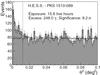 |
Fig. 1 Distribution of the squared angular distance of γ-ray candidate events around the position of PKS 1510−089. The angular distribution (in terms of θ2, the square of the angular distance between the source position and the reconstructed arrival direction) of events around the position of PKS 1510−089 is shown. On-source (signal+background) events are shown as hatched histogram, whereas the off-source (background) events are shown as points with error bars. The on-source region is defined by a |

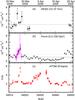 |
Fig. 2 Multiwavelength light curves of PKS 1510−089 for the period between MJD 54 910 to MJD 54 951 in terms of integral fluxes in the respective bands along with the 1σ error bars. Panel a) shows the VHE light curve (one day bins) from H.E.S.S. The horizontal line is obtained by fitting a constant-source model to the data. Panel b) displays the HE light curve derived from Fermi-LAT data. The black open circles show the integrated fluxes in one day bins, whereas a finer binning of 4 h is shown in magenta. The solid line is the average level, and the dashed line is the threshold level used for deriving a flare spectrum during the high state around MJD 54 917. In panel c) the R-band optical fluxes measured with ATOM are shown. |
The VHE light curve (in 1 day bins) is shown in the top panel of Fig. 2. The best-fit integral flux (>0.15 TeV), obtained by fitting a constant-flux model to the light curve, is (8.0 ± 1.6) × 10-12 cm-2 s-1 (χ2 = 20.4 for 11 degrees of freedom). The χ2 test for variability, i.e. for a null hypothesis that the flux is constant, yields a p - value ≈ 0.11 for this value of the χ2 test statistic. This is therefore insufficient evidence to claim statistically significant variability (at a 99% confidence level). Because a few bins in the light curve have low statistics (fewer than 10 counts in the source region and/or background region), the appropriate p - value was derived from simulations of a large number (~ 105) of light curves. An average flux of 8.0 × 10⁻¹² cm-2 s-1 was assumed, and the actual exposure times and instrument effective area in each bin were taken into account. All bins could be thus considered in the test for variability.
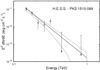 |
Fig. 3 VHE spectrum of PKS 1510−089 measured with the H.E.S.S. instrument, during March 2009. The solid line is the best-fit power law obtained using the forward-folding method (see text for details). The butterfly is the 68% confidence band, and the points with errorbars (1σ statistical errors) are the energy flux. Arrows denote the 99% C.L. upper limits. |
To get the best spectral reconstruction, an additional quality criterion was applied, only those data that were taken with the full array of 4 telescopes were accepted (see Table 1, second row). A total of 6.7 h of good quality 4-telescope data were taken during all observations, yielding 159 γ-ray candidates from the source direction and a statistical significance of 8.2σ. The energy spectrum is derived using a forward-folding technique (Piron et al. 2001). The analysis threshold, Ethr ≈ 0.15 TeV, is given by the energy at which the effective area falls to 10% of its maximum value. For these observations the maximum of the measured differential rate is also at this energy. The likelihood maximization for a power-law hypothesis, dN/dE = N0(E/E0)− Γ, in the energy range 0.15 TeV–1.0 TeV, yields a spectral index of Γ = 5.4 ± 0.7stat ± 0.3sys and a normalization constant of N0 = (1.1 ± 0.2stat ± 0.2sys) × 10-10 cm-2 s-1 TeV-1 at the decorrelation energy, E0 = 0.18 TeV (equivalent to a χ2 of 10.3 with 7 degrees of freedom). The spectral slope is steep compared to other VHE detected blazars, for example, cf. Γ = 4.11 ± 0.68stat for 3C 279 (Albert et al. 2008). The reconstructed H.E.S.S. spectrum is shown in Fig. 3. The integral flux, I(0.15 TeV < E < 1.0 TeV) = (1.0 ± 0.2stat ± 0.2sys) × 10-11 cm-2 s-1 corresponds to ≈3% of the Crab Nebula flux in the same band. Fitting a broken-power-law or a power law with an exponential cutoff does not give a better fit. A spectrum obtained from the entire H.E.S.S. data (first row in Table 1) is compatible with the spectrum derived from the high-quality 4-telescope data, within the statistical errors. The results have been cross-checked using a different analysis method based on multivariate analysis technique (see Ohm et al. 2009, and the references therein), and an independent calibration procedure (Aharonian et al. 2006b).
2.2. Fermi-LAT
It is desirable to compare the VHE spectrum to the Fermi-LAT (Atwood et al. 2009) spectrum during the contemporaneous period. While the Fermi-LAT team has published a spectrum for this source from this period, the integration period used (~1 month) is much larger than the shortest flaring timescale seen by Fermi (Abdo et al. 2010a). The intention here is to obtain a spectrum for the highest state within the Fermi-LAT flares (as defined in Abdo et al. 2010a) that is contemporaneous with HESS observations. Thus the Fermi-LAT data were analyzed using the publicly available Fermi Science Tools1 (v9r23p1-fssc-20111006) and the P7SOURCE_V6 instrument response functions. The light curve over a contemporaneous period as the H.E.S.S. observations is produced by a binned likelihood analysis retaining photons (the source class events) with energies between 200 MeV and 100 GeV from a region of interest of a radius of 10° around the position of PKS 1510−089. All sources from the Fermi-LAT two-years point source catalog (2FGL; Nolan et al. 2012) within an angular distance of 15° of PKS 1510−089 were modeled simultaneously. Pass 7 models2 of the Galactic and extragalactic backgrounds were used. For these two diffuse backgrounds, the normalizations are treated as free parameters in the likelihood analysis. As mentioned before the Fermi-LAT spectrum of this source is best described by a curved log parabola model (Abdo et al. 2010a). Therefore, a log parabola model is used for the source in the likelihood analysis, using the gtlike tool, with the normalization and spectral parameters left free. The light curve derived between MJD 54 909.5 and MJD 54 951.5 is shown in Fig. 2, middle panel. The average (daily binned) integral flux between 200 MeV–100 GeV is (1.26 ± 0.03) × 10-6 cm-2 s-1. Two flares are evident, one centered around MJD 54 916, and the second centered around MJD 54 948. Whereas the H.E.S.S. observations during the first HE flare had good coverage and data quality, the H.E.S.S. observations of the second HE flare commenced only after the HE flare had peaked. A finer binning of 4 h was used around MJD 54 916 to precisely trace the development of the flare.
To characterize the range of variations in the HE band, spectra were extracted over two different epochs from Fermi-LAT data. A spectrum for the long-term average state was derived from the first two years of Fermi-LAT data and a second spectrum was extracted for the high state centered around MJD 54 916. The region of interest, the sources modeled together in the binned likelihood analysis, and the parametrization of the source and the background were identical to that used for the light curve generation. The long-term average spectrum was derived from the data taken between MJD 54 682–MJD 55 412 (i.e., between 04.08.2008–04.08.2010) for energies above 200 MeV using a binned likelihood analysis. This results in a total test statistic (TS, e.g., see Mattox et al. 1996) of 29 440.8. The likelihood analysis was applied in an iterative way, such that the parameters of the 2FGL sources within 15° of PKS 1510−089, and the spectral-shape parameters of PKS 1510−089 are fixed in successive steps, leaving only the normalizations of the source and the two diffuse background components free to vary in the last step. The best-fit values for the log-parabola model (dN/dE = n0 [E/E0] − α − β ln [E/E0]) are – a normalization of n0 = (1.41 ± 0.02) × 10-9 cm-2 s-1 MeV-1, and slope parameters of α = 2.21 ± 0.03 and β = 0.083 ± 0.011. The choice of the reference energy, E0, does not affect the spectral shape and was thus fixed at 260 MeV. These parameters are consistent with the average spectrum presented in Abdo et al. (2010a). A spectrum in logarithm bins in energy (using a log-parabola source model) is also derived for the same period. The average and the energy-binned spectrum are shown in Fig. 4, left panel. A Fermi-LAT spectrum that is strictly simultaneous to the H.E.S.S. spectrum (that is derived from a total exposure of 6.7 h, with gaps in the observations, as well as varying live times for individual exposures) cannot be constructed, because an integration period of at least a few days of Fermi observations is required to derive a meaningful spectrum. Moreover, the H.E.S.S. data used for spectral analysis were spread over a period of 8 days, MJD 54 910–MJD 54 918, during which large flux variations were seen at the Fermi-LAT energies. Because nearly half of the H.E.S.S. exposure was during the brightest phase of the GeV-flare centered around MJD 54 916, the Fermi-LAT data during this period were used to derive a spectrum representing the brightest HE flux state, contemporaneous to the H.E.S.S. observations. Data taken between MJD 54 914.8 to MJD 54 917.5 were used, where the flux points in the Fermi-LAT light curve (in 4-h bins) were above a threshold flux of 2.0 × 10⁻⁶ cm-2 s-1 (see Fig. 2). This threshold flux was chosen to ensure adequate statistics to construct spectral bins reaching at least 10 GeV. The analysis of this data-set yielded a total TS = 2354.0, with the best-fit values for a log-parabola model given by a normalization of n0 = (10.5 ± 0.7) × 10-9 cm-2 s-1 MeV-1, and slope parameters of α = 1.81 ± 0.13 and β = 0.161 ± 0.048 (reference energy fixed at 260 MeV). The corresponding energy-binned spectrum is shown in Fig. 4 (left panel). This is roughly an order of magnitude brighter than the average flux, though it should be noted that the spectrum is biased towards the low-energy bins because of the lack of statistics at higher energies.
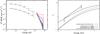 |
Fig. 4 HE and VHE spectra of PKS 1510−089 measured with Fermi-LAT and H.E.S.S., and upper limits on the EBL induced opacity. Left: the filled butterfly shows the H.E.S.S. spectrum as a 1σ confidence band; the blue and red butterflies shows the spectrum corrected for EBL absorption, using the low model for the EBL from Gilmore et al. (2009) and the upper-limit EBL model from Aharonian et al. (2006a) respectively. The triangles show the long-term average Fermi-LAT spectrum, with error bars denoting 1σ statistical errors; the solid curve is the log-parabola model obtained from a binned likelihood analysis of these data (see text for details). The open squares show the Fermi-LAT spectrum derived from the integration period between MJD 54 914.8 and MJD 54 917.5 (error bars illustrate 1σ statistical errors). Arrows denote upper limits on the flux for those bins where insufficient statistics prohibits a flux measurement. The dashed curve is obtained by re-normalizing the long-term average Fermi-LAT spectrum to the level of the high-flux state. Right: upper limits on the EBL opacity derived from spectral measurements of PKS 1510−089 compared to published models. The solid line with arrows at both ends shows the maximum optical depth, corresponding to upper limits on the EBL. For comparison the opacity corresponding to the previously published H.E.S.S. upper-limit EBL model Aharonian et al. (2006a), the Franceschini et al. (2008) model and the low model from Gilmore et al. (2009) are shown. |
2.3. ATOM
The Automatic Telescope for Optical Monitoring (ATOM), Hauser et al. (2004), is a 1 m class optical telescope, located at the H.E.S.S. site. PKS 1510−089 is regularly observed with ATOM. From the onset of the H.E.S.S. observation campaigns, the frequency of optical observations was increased to four observations in the R-band (~640 nm) per night. The R-band light curve, with 500 s exposure per point, not corrected for galactic extinction, is shown in Fig. 2. The optical light curve shows clear and pronounced variability (a reduced χ2 = 55.3, with 117 degrees of freedom from fitting a constant-source model, and the highest flux deviating more than 20σ away from the period average). A prominent flare centered around MJD 54 917 was observed, with another flare occurring after MJD 54 925 that could not be followed up with H.E.S.S. observations because it happened around a full-Moon phase when H.E.S.S. does not operate. A third brightening was seen around MJD 54 946.
These observations show PKS 1510−089 in a relatively high state compared to its average optical brightness, measured with ATOM, between May 2007 and August 2009. For example, in the R-band, compared to the long-term average flux of 1.862 ± 0.004 mJy, the average during the H.E.S.S. observations was 2.597 ± 0.009 mJy and a maximum measured flux of 5.724 ± 0.150 mJy.
3. Discussion
The VHE γ-ray flux of distant (z ≳ 0.1) blazars suffer significant extinction due to pair-production on the diffuse UV-IR photon field in the intergalactic medium (Nikishov 1962; Gould & Schréder 1966). This phenomenon can be used to derive upper limits on the photon density of the UV-IR part of the EBL (e.g., Aharonian et al. 2006a; Mazin & Raue 2007).
Here upper limits are derived by comparing the VHE spectra measured with H.E.S.S. to an extrapolation of the contemporaneous HE spectral measurements obtained with Fermi-LAT, following the procedures in, e.g., Georganopoulos et al. (2010), Aleksić et al. (2011) and Meyer et al. (2012). Modifying Eq. (2) from Aleksić et al. (2011), to include the effect of systematic errors, the 95% confidence upper limit on the EBL, expressed in terms of the optical depth, τmax, is given by ![Mathematical equation: \begin{equation} \label{Eq1} \tau_{\mathrm{max}}(E) = \ln \left[\frac{F_{\mathrm{int}}(E)}{(1-\varepsilon)\times(F_{\mathrm{obs}}(E) - 1.64 \times \Delta F_{\mathrm{obs}}(E))} \right], \end{equation}](/articles/aa/full_html/2013/06/aa21135-13/aa21135-13-eq97.png) (1)where Fobs(E) is the measured flux, ΔFobs(E) is the corresponding 1σ statistical error, Fint(E) is the assumed unattenuated intrinsic flux and ε is the systematic error expressed as a fraction of the measured flux. For a steep spectrum this systematic error (i.e. the uncertainty in the absolute normalization of the flux) is ~25% (i.e. ε = 0.25). The systematic error is conservatively considered as a net bias in the flux measurements. It is the factor by which Fobs(E) could overestimate the true flux. The estimation of τmax in Eq. (1) therefore involves a correction factor of (1 − ε). The extrapolation of the HE spectrum measured with Fermi-LAT into the VHE regime is considered as an estimate for the unattenuated spectrum. The large variations in the HE light curve during the H.E.S.S. observing period require the need of contemporaneous spectral measurements. As already mentioned, a strictly simultaneous Fermi-LAT spectrum corresponding only to the short exposure of H.E.S.S. (Row 2 of Table 1) cannot be obtained because of low statistics in the Fermi-LAT data. Even the spectrum obtained during the high flux state (integrated over 2.7d, centered around MJD 54 916) does not provide sufficient statistics at the high-energy end. Therefore, a conservative estimate resulting in the highest possible upper limit on the opacity is derived by re-normalizing the long-term average Fermi-LAT spectrum to the level of the high-flux state (dashed curve in Fig.4, left panel). This is justified because the long-term spectrum gives the best available description of the HE spectral shape up to the highest GeV energies, and changes in spectral shape during flares are small3. This scaled-up spectrum is extrapolated to the VHE regime to estimate the unattenuated flux, Fint(E), used in Eq. (1). It is assumed that the spectrum smoothly extends from the HE to the VHE band, without spectral breaks or cutoffs. Any intrinsic spectral breaks resulting in lower fluxes at higher energies would yield a lower opacity from EBL attenuation. These assumptions along with the above mentioned considerations (the inclusion of systematic errors on the H.E.S.S. flux and the selection of the intrinsic spectral shape consistent with the brightest HE flux state) give firm upper limits to the EBL opacity. Other sources of opacity, e.g., absorption due to internal photon fields from the BLR or the dusty torus (Wagner et al. 1995), would decrease the contribution from EBL extinction to the overall opacity and thus the previous statement still holds. The EBL upper limits derived using Eq. (1) are shown in Fig. 4, right panel. The EBL limits from this distant FSRQ and the limits in Aharonian et al. (2006a), that are derived from BL Lac type objects that are relatively nearby, are at a comparable level.
(1)where Fobs(E) is the measured flux, ΔFobs(E) is the corresponding 1σ statistical error, Fint(E) is the assumed unattenuated intrinsic flux and ε is the systematic error expressed as a fraction of the measured flux. For a steep spectrum this systematic error (i.e. the uncertainty in the absolute normalization of the flux) is ~25% (i.e. ε = 0.25). The systematic error is conservatively considered as a net bias in the flux measurements. It is the factor by which Fobs(E) could overestimate the true flux. The estimation of τmax in Eq. (1) therefore involves a correction factor of (1 − ε). The extrapolation of the HE spectrum measured with Fermi-LAT into the VHE regime is considered as an estimate for the unattenuated spectrum. The large variations in the HE light curve during the H.E.S.S. observing period require the need of contemporaneous spectral measurements. As already mentioned, a strictly simultaneous Fermi-LAT spectrum corresponding only to the short exposure of H.E.S.S. (Row 2 of Table 1) cannot be obtained because of low statistics in the Fermi-LAT data. Even the spectrum obtained during the high flux state (integrated over 2.7d, centered around MJD 54 916) does not provide sufficient statistics at the high-energy end. Therefore, a conservative estimate resulting in the highest possible upper limit on the opacity is derived by re-normalizing the long-term average Fermi-LAT spectrum to the level of the high-flux state (dashed curve in Fig.4, left panel). This is justified because the long-term spectrum gives the best available description of the HE spectral shape up to the highest GeV energies, and changes in spectral shape during flares are small3. This scaled-up spectrum is extrapolated to the VHE regime to estimate the unattenuated flux, Fint(E), used in Eq. (1). It is assumed that the spectrum smoothly extends from the HE to the VHE band, without spectral breaks or cutoffs. Any intrinsic spectral breaks resulting in lower fluxes at higher energies would yield a lower opacity from EBL attenuation. These assumptions along with the above mentioned considerations (the inclusion of systematic errors on the H.E.S.S. flux and the selection of the intrinsic spectral shape consistent with the brightest HE flux state) give firm upper limits to the EBL opacity. Other sources of opacity, e.g., absorption due to internal photon fields from the BLR or the dusty torus (Wagner et al. 1995), would decrease the contribution from EBL extinction to the overall opacity and thus the previous statement still holds. The EBL upper limits derived using Eq. (1) are shown in Fig. 4, right panel. The EBL limits from this distant FSRQ and the limits in Aharonian et al. (2006a), that are derived from BL Lac type objects that are relatively nearby, are at a comparable level.
Owing to their higher bolometric luminosities FSRQs are detected up to larger distances than BL Lacs. Furthermore, due to the bright emission lines in the spectrum of these objects, which the BL Lacs lack by definition, the redshifts of FSRQs can be accurately measured. Thus the potential of putting strong constraints on the EBL extinction is very promising with FSRQs. However, in the case of PKS 1510−089, other factors currently offset this potential. The H.E.S.S. spectrum turns out to be steep as expected for a high redshift source. This results in a slightly higher systematic error of 25% on the VHE flux measurements (cf. ~20% for a Crab-nebula-like spectrum, index ~2.4, Aharonian et al. 2006b). Furthermore, this sharply falling spectrum makes it difficult to collect good statistics at energies >0.5 TeV and hence the statistical errors in this energy range are also high. The combined effect of the large statistical and systematic errors in the VHE spectrum (denoted by ΔFobs and ε respectively in Eq. (1)), because of the steep VHE spectral slope of this source, limits the effectiveness of the method used above. Thus only weak EBL limits could be derived. Another aspect that limits the ability to put strong EBL constraints is the uncertainty in the intrinsic spectral shape. For the observations presented here there is insufficient evidence for claiming variability in the VHE band. However, because the unabsorbed HE band is highly variable (time scale of hours) it is difficult to obtain an accurate description of the intrinsic spectral shape (Fint in Eq. (1)) due to the typically multi-day integration time required, hence making it difficult to put stricter EBL constraints. For example, if the estimated Fint at the lowest energies were estimated to be 20% less than the value used, which is perfectly plausible when comparing to the factor of ~4 variations in the Fermi fluxes seen during this period, the EBL UL from this source calculated as above would have been more constraining than the Aharonian et al. (2006a) limits. With more multiwavelength monitoring of bright FSRQs, such as PKS 1510−089 and other FSRQs that have less steep VHE spectrum, it could be possible to obtain a HE and VHE spectrum when the fluxes in neither band varies. This of course is better done with more sensitive Cherenkov telescopes, such as the H.E.S.S. II telescope array, which should provide richer statistics due to their higher sensitivities and larger energy coverage. This should allow putting stronger constraints on the EBL extinction by comparing their quiescent-state HE and VHE spectrum.
The luminous broad line emission in the optical-UV band as well as the thermal UV excess in PKS 1510−089 indicate an intense internal photon field. This can in principle cause substantial absorption of VHE γ-rays within the BLR radius, or due to the reprocessed disk emission from the dusty torus at larger distances from the accretion disk. The H.E.S.S. detection of this source implies a low optical depth in the VHE emitting region. This can be tentatively explained by hypothesizing that the VHE emitting region is in an optically thin part of the jet, presumably far outside the BLR, see e.g., Tanaka et al. (2011) and Tavecchio et al. (2011) for discussion on the FSRQ PKS 1222+216. It should be noted that in the study made in Poutanen & Stern (2010), where a search is made for signature features of BLR absorption in the HE spectrum of several of the brightest FSRQs detected by Fermi, the HE spectrum of PKS 1510−089 is consistent with a negligible amount of absorption due to line emission in BLR clouds. This is consistent with the hypothesis that the γ-ray emitting zone is in an optically thin region. A detailed discussion of the internal opacity is beyond the scope of this work.
4. Summary
VHE emission was detected from the flat-spectrum radio quasar PKS 1510−089 with a statistical significance of 9.2 standard deviations in 15.8 h of H.E.S.S. data taken during March and April 2009. An integral flux, in the energy regime between 0.15–1.0 TeV, of (1.0 ± 0.2stat ± 0.2sys) × 10-11 cm-2 s-1 is measured, which is ≈3% of the Crab Nebula flux. The spectrum is extremely steep with a photon index of Γ = 5.4 ± 0.7stat ± 0.3sys for a power-law hypothesis.
There is insufficient evidence to claim significant variability in the H.E.S.S. data. However, the multifrequency data on PKS 1510−089 during the H.E.S.S. observation period shows clear and pronounced variability in the HE and optical bands. Using both the Fermi-LAT and H.E.S.S. γ-ray spectrum, from 200 MeV to 1 TeV, upper limits on the optical depth due to the EBL are derived. The EBL-limits in this work are comparable with the limits in Aharonian et al. (2006a), that were derived from BL Lac objects that are relatively nearby. FSRQs, such as PKS 1510−089, due to their higher luminosities compared to BL Lacs, can in principle, allow us to probe the EBL density to relatively higher redshifts. With the upcoming H.E.S.S. II telescope array more precise measurements of the spectra of distant blazars are expected, which will allow us to put stronger constraints on the EBL.
Abdo et al. (2010a) find a harder when brighter trend in the Fermi-LAT spectrum when the flux above 0.2 GeV is ≳ 2.4 × 10⁻⁷ cm-2 s-1. However, the change in the photon index is small, ≲0.2.
Acknowledgments
The support of the Namibian authorities and of the University of Namibia in facilitating the construction and operation of H.E.S.S. is gratefully acknowledged, as is the support by the German Ministry for Education and Research (BMBF), the Max Planck Society, the German Research Foundation (DFG), the French Ministry for Research, the CNRS-IN2P3 and the Astroparticle Interdisciplinary Programme of the CNRS, the UK Science and Technology Facilities Council (STFC), the IPNP of the Charles University, the Czech Science Foundation, the Polish Ministry of Science and Higher Education, the South African Department of Science and Technology and National Research Foundation, and by the University of Namibia. We appreciate the excellent work of the technical support staff in Berlin, Durham, Hamburg, Heidelberg, Palaiseau, Paris, Saclay, and in Namibia in the construction and operation of the equipment. We acknowledge the information provided by the Fermi-LAT collaboration on the Fermi-LAT measured fluxes of PKS 1510−089 during the 2009 flaring episodes, which helped scheduling of the H.E.S.S. observations presented here. This work has been partially supported by the International Max Planck Research School (IMPRS) for Astronomy & Cosmic Physics at the University of Heidelberg. We acknowledge the anonymous referee for providing useful suggestions that improved the clarity.
References
- Abdo, A. A., Ackermann, M., Ajello, M., et al. (Fermi Collaboration) 2009, ApJ, 700, 597 [NASA ADS] [CrossRef] [Google Scholar]
- Abdo, A. A., Ackermann, M., Agudo, I., et al. (Fermi Collaboration) 2010a, ApJ, 721, 1425 [NASA ADS] [CrossRef] [Google Scholar]
- Abdo, A. A., Ackermann, M., Ajello, M., et al. (Fermi Collaboration) 2010b, ApJS, 188, 405 [NASA ADS] [CrossRef] [Google Scholar]
- Aharonian, F., Akhperjanian, A. G., Bazer-Bachi, A. R., et al. (H.E.S.S. Collaboration) 2006a, Nature, 440, 1018 [NASA ADS] [CrossRef] [PubMed] [Google Scholar]
- Aharonian, F., Akhperjanian, A. G., Bazer-Bachi, A. R., et al. (H.E.S.S. Collaboration) 2006b, A&A, 457, 899 [NASA ADS] [CrossRef] [EDP Sciences] [Google Scholar]
- Albert, J., Aliu, E., Anderhub, H., et al. (MAGIC Collaboration) 2008, Science, 320, 1752 [NASA ADS] [CrossRef] [PubMed] [Google Scholar]
- Aleksić, J., Antonelli, L. A., Antoranz, P., et al. (MAGIC Collaboration) 2011, ApJ, 730, L8 [NASA ADS] [CrossRef] [Google Scholar]
- Aller, M. F., Aller, H. D., & Hughes, P. A. 2003, ApJ, 586, 33 [NASA ADS] [CrossRef] [Google Scholar]
- Andrei, A. H., Souchay, J., Zacharias, N., et al. 2009, A&A, 505, 385 [NASA ADS] [CrossRef] [EDP Sciences] [MathSciNet] [Google Scholar]
- Atwood, W. B., Abdo, A. A., Ackermann, M., et al. 2009, ApJ, 697, 1071 [NASA ADS] [CrossRef] [Google Scholar]
- Berge, D., Funk, S., Hinton, J., et al. 2007, A&A, 466, 1219 [Google Scholar]
- Burbidge, E. M., & Kinman, T. D. 1966, ApJ, 145, 654 [NASA ADS] [CrossRef] [Google Scholar]
- Cutini, S., Hays, E., & the Fermi Large Area Telescope Collaboration 2009, ATel, 2033 [Google Scholar]
- D’Ammando, F., Vercellone, S., Tavani, M., et al. 2009, ATel, 1957 [Google Scholar]
- de Naurois, M., & Rolland, L. 2009, Astropart. Phys., 32, 231 [NASA ADS] [CrossRef] [Google Scholar]
- Donea, A.-C., & Protheroe, R. J. 2003, Astropart. Phys., 18, 377 [Google Scholar]
- Franceschini, A., Rodighiero, G., & Vaccari, M. 2008, A&A, 487, 837 [NASA ADS] [CrossRef] [EDP Sciences] [Google Scholar]
- Georganopoulos, M., Finke, J. D., & Reyes, L. C. 2010, ApJ, 714, L157 [NASA ADS] [CrossRef] [Google Scholar]
- Gilmore, R., Madau, P., Primack, J. R., et al. 2009, MNRAS, 399, 1694 [Google Scholar]
- Gould, R. J., & Schréder, G. P. E. 1966, Phys. Rev. Lett., 16, 252 [Google Scholar]
- Hartman, R. C., Bertsch, D. L., Bloom, S. D., et al. 1999, ApJS, 123, 79 [NASA ADS] [CrossRef] [Google Scholar]
- Hauser, M., Möllenhoff, C., Pühlhofer, G., et al. 2004, Astron. Nachr., 325, 659 [Google Scholar]
- Hinton, J. 2004, New. Astron. Rev., 48, 331 [Google Scholar]
- Homan, D. C., Ojha, R., Wardle, J. F. C., et al. 2001, ApJ, 549, 840 [NASA ADS] [CrossRef] [Google Scholar]
- Homan, D. C., Wardle, J. F. C., Cheung, C. C., et al. 2002, ApJ, 580, 742 [NASA ADS] [CrossRef] [Google Scholar]
- Jorstad, S. G., Marscher, A. P., Lister, M. L., et al. 2005, AJ, 130, 1418 [NASA ADS] [CrossRef] [Google Scholar]
- Jorstad, S. G., Marscher, A. P., Aller, M. F., & Balonek, T. J. 2006, AGN Variability from X-Rays to Radio Waves, ASP Conf. Ser., 360, 169 [NASA ADS] [Google Scholar]
- Kalberla, P. M. W., Burton, W. B., Hartmann, D., et al. 2005, A&A, 440, 775 [NASA ADS] [CrossRef] [EDP Sciences] [Google Scholar]
- Kataoka, J., Madejski, G., Sikora, M., et al. 2008, ApJ, 672, 787 [NASA ADS] [CrossRef] [Google Scholar]
- Larionov, V. M., Villata, M., Raiteri, C. M., et al. 2009, ATel, 1990 [Google Scholar]
- Li, T.-P., & Ma, Y.-Q. 1983, ApJ, 272, 317 [NASA ADS] [CrossRef] [Google Scholar]
- Liu, H. T., & Bai, J. M. 2006, ApJ, 653, 1089 [NASA ADS] [CrossRef] [Google Scholar]
- Malkan, M. A., & Moore, R. L. 1986, ApJ, 300, 216 [NASA ADS] [CrossRef] [Google Scholar]
- Mattox, J. R., Bertsh, D. L., Chiang, J., et al. 1996, ApJ, 461, 396 [NASA ADS] [CrossRef] [Google Scholar]
- Marscher, A. P., Jorstad, S. G., Larinov, V. M., et al. 2010, ApJ, 710, L126 [NASA ADS] [CrossRef] [Google Scholar]
- Mazin, D., & Raue, M. 2007, A&A, 471, 439 [NASA ADS] [CrossRef] [EDP Sciences] [Google Scholar]
- Mead, A. R. G., Ballard, K. R., Brand, P. W. J. L., et al. 1990, A&AS, 83, 183 [NASA ADS] [Google Scholar]
- Meyer, M., Raue, M., Mazin, D., et al. 2012, A&A, 542, A59 [NASA ADS] [CrossRef] [EDP Sciences] [Google Scholar]
- Nikishov, A. I. 1962, Sov. Phys. J. Exp. Theor. Phys., 14, 393 [Google Scholar]
- Nolan, P. A., Abdo, A. A., Ackermann, M., et al. (Fermi Collaboration) 2012, ApJS, 199, 31 [NASA ADS] [CrossRef] [Google Scholar]
- Ohm, S., van Eldik, C., & Egberts, K. 2009, Astropart. Phys., 31, 383 [NASA ADS] [CrossRef] [Google Scholar]
- Piron, F., Djannati-Ataï, A., Punch, M., et al. 2001, A&A, 374, 895 [NASA ADS] [CrossRef] [EDP Sciences] [Google Scholar]
- Poutanen, J., & Stern, B. 2010, ApJ, 717, L118 [Google Scholar]
- Pucella, G., D’Ammando, F., Tavani, M., et al. 2009, ATel, 1968 [Google Scholar]
- Salamon, M. H., & Stecker, F. W. 1998, ApJ, 493, 547 [NASA ADS] [CrossRef] [Google Scholar]
- Stockman, H. S., Moore, R. L., & Angel, J. R. P. 1984, ApJ, 279, 485 [NASA ADS] [CrossRef] [Google Scholar]
- Tadhunter, C. N., Morganti, R., Di Serego-Alighieri, S., et al. 1993, MNRAS, 263, 999 [NASA ADS] [CrossRef] [Google Scholar]
- Tavecchio, F., Becerra-Gonzalez, J., Ghisellini, G., et al. 2011, A&A, 534, A86 [NASA ADS] [CrossRef] [EDP Sciences] [Google Scholar]
- Tanaka, Y. T., Stawarz, Ł., Thompson, D. J., et al. 2011, ApJ, 733, 19 [NASA ADS] [CrossRef] [Google Scholar]
- Vercellone, S., D’Ammando, F., Pucella, G., et al. 2009, ATel, 1976 [Google Scholar]
- Villata, M., Raiteri, C. M., Larionov, V. M., et al. 2009, ATel, 1988 [Google Scholar]
- Wagner, S. J., & Witzel, A. 1995, ARA&A, 33, 163 [NASA ADS] [CrossRef] [Google Scholar]
- Wagner, S. J., Camenzind, M., Dreissigacker, O., et al. 1995, A&A, 298, 688 [NASA ADS] [Google Scholar]
All Tables
All Figures
|
Fig. 1 Distribution of the squared angular distance of γ-ray candidate events around the position of PKS 1510−089. The angular distribution (in terms of θ2, the square of the angular distance between the source position and the reconstructed arrival direction) of events around the position of PKS 1510−089 is shown. On-source (signal+background) events are shown as hatched histogram, whereas the off-source (background) events are shown as points with error bars. The on-source region is defined by a |
| In the text | |
|
Fig. 2 Multiwavelength light curves of PKS 1510−089 for the period between MJD 54 910 to MJD 54 951 in terms of integral fluxes in the respective bands along with the 1σ error bars. Panel a) shows the VHE light curve (one day bins) from H.E.S.S. The horizontal line is obtained by fitting a constant-source model to the data. Panel b) displays the HE light curve derived from Fermi-LAT data. The black open circles show the integrated fluxes in one day bins, whereas a finer binning of 4 h is shown in magenta. The solid line is the average level, and the dashed line is the threshold level used for deriving a flare spectrum during the high state around MJD 54 917. In panel c) the R-band optical fluxes measured with ATOM are shown. |
| In the text | |
|
Fig. 3 VHE spectrum of PKS 1510−089 measured with the H.E.S.S. instrument, during March 2009. The solid line is the best-fit power law obtained using the forward-folding method (see text for details). The butterfly is the 68% confidence band, and the points with errorbars (1σ statistical errors) are the energy flux. Arrows denote the 99% C.L. upper limits. |
| In the text | |
|
Fig. 4 HE and VHE spectra of PKS 1510−089 measured with Fermi-LAT and H.E.S.S., and upper limits on the EBL induced opacity. Left: the filled butterfly shows the H.E.S.S. spectrum as a 1σ confidence band; the blue and red butterflies shows the spectrum corrected for EBL absorption, using the low model for the EBL from Gilmore et al. (2009) and the upper-limit EBL model from Aharonian et al. (2006a) respectively. The triangles show the long-term average Fermi-LAT spectrum, with error bars denoting 1σ statistical errors; the solid curve is the log-parabola model obtained from a binned likelihood analysis of these data (see text for details). The open squares show the Fermi-LAT spectrum derived from the integration period between MJD 54 914.8 and MJD 54 917.5 (error bars illustrate 1σ statistical errors). Arrows denote upper limits on the flux for those bins where insufficient statistics prohibits a flux measurement. The dashed curve is obtained by re-normalizing the long-term average Fermi-LAT spectrum to the level of the high-flux state. Right: upper limits on the EBL opacity derived from spectral measurements of PKS 1510−089 compared to published models. The solid line with arrows at both ends shows the maximum optical depth, corresponding to upper limits on the EBL. For comparison the opacity corresponding to the previously published H.E.S.S. upper-limit EBL model Aharonian et al. (2006a), the Franceschini et al. (2008) model and the low model from Gilmore et al. (2009) are shown. |
| In the text | |
Current usage metrics show cumulative count of Article Views (full-text article views including HTML views, PDF and ePub downloads, according to the available data) and Abstracts Views on Vision4Press platform.
Data correspond to usage on the plateform after 2015. The current usage metrics is available 48-96 hours after online publication and is updated daily on week days.
Initial download of the metrics may take a while.