| Issue |
A&A
Volume 554, June 2013
|
|
|---|---|---|
| Article Number | A46 | |
| Number of page(s) | 14 | |
| Section | Stellar atmospheres | |
| DOI | https://doi.org/10.1051/0004-6361/201220840 | |
| Published online | 31 May 2013 | |
Atmospheric dynamics in RR Lyrae stars
The Blazhko effect
Observatoire de Haute-Provence – CNRS/PYTHEAS/Université d’Aix-Marseille, 04870 Saint Michel l’Observatoire, France
e-mail: denis.gillet@oamp.fr
Received: 3 December 2012
Accepted: 29 March 2013
Context. Discovered in 1907, the Blazhko effect is a modulation of the light variations of about half of the RR Lyr stars. It has remained unexplained for over 100 years, despite more than a dozen proposed explanations. Today it represents an ongoing challenge in variable-star research.
Aims. We propose a new explanation. It is based on the observation that Blazhko stars seem to be located in the region of the instability strip where fundamental and first overtone modes are excited at the same time.
Methods. An analysis of nonlinear and nonadiabatic pulsation models of RR Lyrae stars shows that a specific shock (called first overtone shock) may be generated by the perturbation of the fundamental mode by the transient first overtone.
Results. The first overtone shock induces a sharp slowdown of the atmospheric layers during their infalling motion. This slowdown in turn affects the compression rate on the deep photospheric layers and the intensity of the κ-mechanism. After an amplification phase, the intensity of the main shock wave before the Blazhko maximum becomes high enough to provoke large radiative losses. These can be at least equal to 70% of the total energy flux of the shock, which induces a small decrease of the effective temperature at each pulsation cycle. In these conditions, when the intensity of the main shock reaches its highest critical value at the Blazhko maximum, it completely desynchronizes the motion of the phostospheric layers. At this point, the atmosphere relaxes and reaches a new synchronous state that occurs at the Blazhko minimum.
Conclusions. The combined effects of these two shocks on the atmosphere cause the Blazhko effect. This effect can only exist if the first overtone mode is excited together with the fundamental mode. Because the involved physical mechanisms are essentially nonlinear (shocks, atmospheric dynamics, radiative losses, mode excitations), the Blazhko process is expected to be unstable and irregular. Consequently, the Blazhko process has a specific random nature that is in contrast with the pulsation of non-Blazhko stars.
Key words: shock waves / stars: atmospheres / stars: variables: RR Lyrae / stars: individual: RR Lyr
© ESO, 2013
1. Introduction
In 1907, the Soviet astronomer Sergey Nikolaevich Blazhko observed for the first time periodic variations in the timing of maximum light for the RR Lyrae star RW Dra (Blazhko 1907). Pragen (1916) and Shapley (1916) had independently discovered that the light curve of RR Lyr was also modulated in amplitude and shape, with a period of about 40 days. This modulation became known as the Blazhko effect. After several decades of dedicated studies of Blazhko stars, the cause of the Blazhko effect is now a long-standing mystery. This secular problem has been recently reviewed by Kolenberg (2012). Since the first explanation by Kluyver (1936), more than ten models have been proposed to explain the amplitude and phase modulations on timescales of days to months that are induced by this effect. Stothers (2006) and Smolec et al. (2011) provided a detailed discussion of the different approaches proposed over the past decades. These include tides in a binary system, resonance between radial modes or between a radial mode and a nonradial mode, or the influence of a magnetic field on the pulsations of the star. The last two explanations have been the most elaborate, but are currently ruled out by observations, as shown by Smolec et al. (2011). For intance, models that require a magnetic field were excluded because all measurements of the mean longitudinal magnetic field resulted in null detections within 3σ (Kolenberg & Bagnulo 2009). Moreover, all these solutions produce a regular variation of modulations occurring in the light and radial velocity curves. However, recent highly accurate space-based observations definitively establish that the Blazhko effect has irregularities. This stochastic nature of the Blazhko effect is therefore an important feature that any future explanation must take into account.
Recently, Stothers (2006, 2010) proposed a new explanation of the Blazhko effect. The modulation is supposed to be caused by changes in the structure of the outer convective zone, generated by an irregular variation of the magnetic field. However, Stothers did not provide an accurate physical reason that would produce the strengthening and weakening of the turbulent convection. To confirm this idea, a quantitative model capable of reproducing the light modulations must be produced. Smolec et al. (2011) presented a simplified model to estimate the validity of Stothers’ idea. To do this, they slightly modified the nonlinear convective pulsation hydrocode proposed by Smolec & Moskalik (2008). They assumed that the intensity of the turbulent convection changes by the periodic variation of a mixing-length parameter α. Thus, this simple model cannot predict quasi-periodic modulation as observed. This model shows that reproducing the modulation of the light curve of RR Lyr requires a variation of about 50% of the mixing length on a timescale shorter than the Blazhko period. Consequently, the question is how rapid (tens of days or less as in the case of SS Cnc (Jurcsik et al. 2006), the shortest known Blazhko period 5.31 days) and strong (50%) changes of the turbulent convective structure are physically possible. Finally, Stothers’ idea requires not only a more a refined model but also a more detailed analysis of his observations.
More recently, Buchler & Kolláth (2011) proposed that the fundamental pulsation mode can become destabilized by a 9:2 resonant interaction with the ninth overtone. Normally high-order pulsation modes such as the 9th are not able to destabilize the fundamental mode limit cycle because they have a strong damping rate. In their hydrodynamical simulations, Szabó et al. (2010) showed that the 9th overtone is a strange mode (or surface mode) i.e., the energy associated with its pulsation is confined to the outer zones of the star. Consequently, its damping rate should be short enough to destabilize the fundamental mode. Using the amplitude equation formalism of Buchler & Goupil (1984), Buchler & Kolláth (2011) showed that this 9:2 resonance causes the modulation observed in Blazhko stars. It can also yield the period doubling (PD) that is observed in a few Blazhko stars. Szabó et al. (2010) observed a strong PD effect in three stars and a weaker one in four stars out of the 14 Blazhko stars observed by the Kepler space telescope. However, the PD effect was not found in the 15 non-Blazhko stars observed with Kepler. Nevertheless, this effect is transient, varies with the Blazhko cycle, and is not observed in all Blazhko cycles.
Continuous and accurate observations of the CoRoT and Kepler space telescopes revealed many new frequencies in addition to the usual RR Lyrae pattern (fundamental and Blazhko periods). These small additional features show that the pulsation of RR Lyrae stars is not limited to the two lowest radial modes, but is more complex than initially suspected. At the Konkoly Observatory, Kolláth and his colleagues are studying this new aspect of the pulsation of these stars, which could be called nonlinear astroseismology of RR Lyrae (Molnár et al. 2012a,b). They note that almost all stars that show additional modes are Blazhko variables. For the first time, they detected the first overtone in RR Lyr, which has a very small amplitude of a few millimagnitudes, which explains why it has remained undetected by ground-based telescopes. In addition, a closer inspection of their nonlinear hydrodynamic models reveals that when three different radial modes are present (the fundamental mode and the first and ninth overtone), a great variety of resonant, nonresonant and chaotic states are observed.
Currently, an intense debate about the physical origin of the Blazhko effect is in progress. We propose a new approach to this effect here. It is based on the fact that the photospheric dynamics of the atmosphere is strongly affected by five strong shocks in each pulsation cycle. We have studied the effects of the interaction of these shocks with atmospheric layers and especially with photospheric ones. In Sect. 2 of this paper, we discuss the pulsating stars that show the Blazhko effect. In Sect. 3, we provide the location of Blazhko stars and non-Blazhko stars in the Hertzsprung-Russell diagram. A new explanation of the Blazhko mechanism is proposed in Sect. 4. Observational clues are investigated in Sect. 5: detection of the first overtone in Blazhko stars, turbulence amplification, helium emission occurrence, UV-excesses, moving bump, variation of the pulsation parameters during the Blazhko cycle, shock amplification phase from Kepler data, amplitudes of Blazhko stars, connection between pulsation and Blazhko periods, irregularities and period doublings, and possible connection of the Blazhko effect to the pulsation mode switch. Finally, some concluding remarks are given in Sect. 6.
2. RR Lyrae stars affected by the Blazhko effect
The RRa, RRb, and RRc Bailey types for RR Lyrae stars were introduced by Bailey (1902) in his study of variable stars in the globular cluster ω Centauri. In his original classification, Bailey fixed the separation between RRa and RRb types to a period of 15 h (0.625 day). RRa and RRb are now usually condensed to just one type, called RRab, because the gradual transition between them made them almost undistinguishable. Thus, depending on the shape of the light curve, at least 90% of RR Lyrae stars are divided into two main subclasses: RRab-type with asymmetric light curves with a fast rise and slower decline, and RRc-type with nearly sinusoidal light curves. RRab are fundamental mode pulsators, RRc are first overtone pulsators. When both the fundamental mode and the first overtone are present, we have double-mode RR Lyrae (RRd) stars. RRe-type are variables in the second overtone mode.
Of the 16 836 stars of the OGLE-III Catalog of Variable Stars (Soszyński et al. 2011) in the Galactic Bulge, 70% are RRab-type stars and 30% are RRc-type stars, while RRd-type stars are quite marginal (0.5%). In the Large Magellanic Cloud, this last number increases to 4% for a total sample of 24,906 RR Lyrae stars (Soszyński et al. 2009). Based on the amplitude equation formalism, Szabó et al. (2004) presented a large-scale survey of the nonlinear pulsations in the RR Lyrae instability strip (hereafter IS). They showed that the IS-region where stable double-mode pulsations occur is very narrow, and that they occur at high masses, unlike the region that contains both RRab and RRc. As a result, it is not surprising that the observed number of RRd stars is so low.
Szeidl (1976) reported that three stars in the Galactic field can be considered as RRc Blazhko stars: TV Boo, BV Aqr, and RU Psc. Olech et al. (1999) showed that three RRc variables in the globular cluster M55 exhibit marked amplitude modulation on a timescale shorter than a week. They thought it unlikely that this behavior would be caused by the Blazhko effect because on certain occasions the observation of the light curve amplitude changes on a timescale of days. Nevertheless, today, these three stars are accepted as RRc of the Blazhko type (Arellano Ferro et al. 2012). Moreover, several variables of this type have been discovered in the LMC, in NGC 6362, and in the OGLE data base. Recently, Arellano Ferro et al. (2012) showed that 66% of the total population of RRc in the globular cluster M53 (NGC 5024) present amplitude and phase modulations typical of the Blazhko effect, while only 37% of RRab are of Blazhko type. The fact that part of the RRc-types exhibit the Blazhko effect is quite surprising. This new detection is mainly due to deep and large surveys for RR Lyrae stars. We expect that the number of Blazhko RRc stars significantly increases in the next few years. Nevertheless, currently, M53 is the globular cluster with the largest number of RRc Blazhko variables, while no RRc stars with the Blazhko effect are known in the globular cluster M5 (Jurcsik et al. 2011a). New observations are necessary to confirm and understand the difference between globular clusters.
Finally, the Blazhko effect could be a common effect among RRc and RRab variables. However, it is not yet established that the physical mechanism causing the Blazhko effect would be exactly the same for RRc and RRab stars. Thus, the RRc stars may or may not exhibit the same Blazhko effect as the RRab stars. Furthermore, as noted by Molnár et al. (2012a,b), the great variety of resonant, nonresonant and chaotic possible states in RR Lyrae stars must be taken into account to explain all observed types of low-amplitude variations such as small modulations. If the Blazhko effect is linked with the interaction of strong shock waves, the intensity of the shocks is certainly lower in RRc than in RRab because we do not observe emission lines of hydrogen in RRc. Therefore, this significant difference should be taken into account when one aims to explain the Blazhko effect in RRc. The OGLE-III Catalog (Soszyński et al. 2009, 2011) shows that the light amplitude of RRc and RRd stars is similar and two to three times lower than the maximum amplitude of RRab.
Until now, the Blazhko effect has not been observed in RRd. This may be an observational bias due to the small number of RRd compared to RRab and RRc. But it is also possible that the coexistence of stable oscillations in the fundamental and first overtone modes during the same pulsation cycle may reduce the development of the shock amplitude. Therefore, a Blazhko effect based on the interaction of strong shock waves should not be possible in double-mode RR Lyrae stars. This is consistent with the fact that RRd do not show hydrogen lines in emission, which are the signature of strong shocks. However, RRc and RRd have similar amplitudes. Accordingly, the possibility of Blazhko RRd stars is not irrefutably excluded because we observe Blazhko RRc stars.
Period-amplitude (Bailey) diagrams for RR Lyrae stars toward the Galactic Bulge (Soszyński et al. 2011) or in the LMC (Soszyński et al. 2009), for instance, show that RRab form a very distinct group with other Bailey-type stars of short periods (RRc, RRd, and RRe). Indeed, these stars have P ≲ 0.45 day, while for RRab, P is between 0.45 and 1 day. RRe variables have lower amplitudes and slightly shorter periods than RRc variables. The amplitudes of the RRab stars are strongly anti-correlated with the period, whereas the amplitudes of the RRc stars have a parabolic distribution. The maximum V-amplitude of short-period RR Lyrae never exceeds 0.7 but can reach up to 1.6 for RRab (Soszyński et al. 2003). Moreover, the amplitude position of a star in the Bailey diagram can be strongly affected by the Blazhko effect (Szeidl 1988), which concerns up to 50% of RR Lyrae stars. Indeed, in the Bailey diagram the highest amplitude of the Blazhko stars always fit the mean distribution of the non-Blazhko stars while the smallest ones induce a high dispersion at lower amplitudes.
The ASAS Catalogue of Variable Stars (Szczygiel & Fabrycky 2007) contains 2212 RR Lyrae from a Galactic survey of 75% of the whole sky with 8 < V < 14 mag. The period analysis of this RR Lyrae sample shows a lack of Blazhko variables with pulsation periods longer than 0.625 day. In addition, the list of well-known Galactic field Blazhko variables (242 stars), recently published by Skarka (2013), confirms this deficiency of Blazhko stars. Indeed, 95% of Blazhko stars have a pulsation period shorter than 0.625 day.
Thus, because the density of RR Lyrae stars with pulsation periods ≲0.625 day and V-amplitudes ≲0.7 is significantly lower, we can estimate that most/almost all RRab Blazhko stars have a high amplitude (0.7 < Δ V < 1.6). This means that strong shocks are necessarily present in their atmosphere. As shown by exemplary light curves of RR Lyrae stars in the LMC published by Soszyński et al. (2003), RRab curves become nearly sinusoidal when P ≳ 0.625 day (see their Fig. 3). We can also expect that the average pulsation period of Blazhko stars is lower than that of non-Blazhko stars. This tendency was already recognized by Preston (1964) in the globular cluster M5 and by Nemec (1985) in six globular clusters, in the Draco dwarf galaxy, and among field variables.
Consequently, because of the completeness of OGLE surveys (Soszyński et al. 2011), we can reintroduce RRa (P ≲ 0.625 day) and RRb (P ≳ 0.625 day) types. Furthermore, almost all Blazhko stars are within the RRa group, while there are virtually no Blazhko stars in the RRb group, as shown by Jurcsik et al. (2011b) for M5. The stiffness of the rising branch of light curves could thus be seen as a signature of strong shocks in the atmosphere of RR Lyrae stars.
Consider the V-band Bailey diagram for RR Lyrae stars published by Soszyński et al. (2003), their Fig. 8. Statistically, the amplitudes of RRab are highest when the observed periods are shortest (P ~ 0.45 day). Consequently, it is plausible that the intensity of the main shock reaches significantly high values for these periods. In this case, emission lines of high intensity should be preferentially observed in RRab stars with short periods. The amplitudes of RRab gradually decreases by up to 0.2 for periods of about 0.70 day. For periods of this length, strong shocks are not observed and Blazhko stars are rare. In RRc stars, shock intensities are expected to be three to four times weaker than in RRab stars (Fokin 2012, priv. comm.). For this reason, we could hypothesize that statistically there is a striking amplitude jump between short-period (RRc) and long-period (RRa) stars near the period 0.45 day. This is what we observe, especially in data from large surveys such as OGLE.
Finally, because currently there are no atmospheric pulsation models of RRc and RRd that produce a comprehensive study of shock wave dynamics, we focus on the cause of the Blazhko effect in RRab, i.e., RRa stars as defined above.
Non-Blazhko stars do not seem to be purely fundamental mode pulsators with perfect stationary light curves. Beyond the primary frequency and its harmonics, additional peaks with small amplitudes have been found (Benkö et al. 2010). A comprehensive and more detailed study of the Kepler non-Blazhko stars would be useful to determine the exact deviations from perfectly periodic pulsation. Nemec et al. (2011) and Benkö et al. (2010) found that KIC 7021124 and V350 Lyr pulsate simultaneously in the fundamental and second-overtone modes. These stars are two special cases among the 19 non-Blazhko stars in the Kepler field.
3. Location of Blazhko stars in the HRD
The location in the Hertzsprung-Russell diagram (hereafter HRD) of RR Lyrae types RRab and RRc is currently a difficult exercise. Indeed, neither the accuracy of the average luminosity ⟨ L ⟩ nor that of the effective temperature ⟨ Teff ⟩ is particularly good because the reddening effect, the metallicity effect, the surface gravity, and the turbulent velocity, among others, affect the relationships employed (Eqs. (10) and (11), Nemec et al. 2011) to determine ⟨ L ⟩ and ⟨ Teff ⟩. Moreover, the amplitude of changes induced by the pulsation during each cycle is high and is not strictly regular from one cycle to the other. Thus, the above relationships derived from stellar evolution models or from stellar pulsation models provide disparate results (see Fig. 13 of Nemec et al. 2011). Furthermore, the blue and red edges of the instability strip are yet to be defined accurately (compare for example those given by Stellingwerf 1975; and Nemec et al. 2011). Nevertheless, apparently the location of non-Blazhko stars is redder and closer to the fundamental mode red-edge than that of Blazhko stars (Fig. 1). With the use of the Kepler space telescope, this HR-diagram, adapted from Fig. 13 of Nemec et al. (2011), shows the location of 19 non-Blazhko stars (squares) and 9 Blazhko stars (circles) with known values for luminosity and effective temperature (see Table 1). Two sets of Horizontal Branch (HB) models (low- and high-metallicity) from Dorman (1992) are given for comparison. The edges of the IS were calculated with the Warsaw linear pulsation code assuming a mass M = 0.65 M⊙. The fundamental mode edges are plotted as solid lines and first overtone mode edges as dashed lines. As proposed by Pietrynski et al. (2010), the pulsational luminosities and masses derived from stellar pulsation models appears to be more accurate than those derived from stellar evolution models because not enough mass loss has been taken into account in the evolution theory. Consequently, we chose the pulsational solution for our star locations in the HRD. Although the number of Blazhko stars used is limited, all are within an intermediate region of the IS in which both the fundamental and the first overtone modes of pulsation are excited at the same time. In contrast, non-Blazhko stars would not be affected at all or only slightly by the first overtone during their pulsation cycle. This trend needs to be confirmed by more detailed observations.
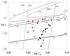 |
Fig. 1 HR diagram adapted from Nemec et al. (2011) showing the locations of the Kepler non-Blazhko RR Lyrae stars (squares) compared with the Blazhko stars (circles) with known luminosity and effective temperature (see Table 1). For non-Blazhko stars, the luminosity was derived from stellar pulsation models, which take into account mass loss in contrast to evolution models. The blue and red edges for the IS were computed using the Warsaw pulsation code. The fundamental mode edges (FBE, FRE) are plotted as solid lines, and first overtone mode edges (FOBE, FORE) as dashed lines. The two sets of HB models (low- and high-metallicity) are taken from Dorman (1992). The numbers on the evolutionary tracks give the masses of evolution models. |
4. Blazhko mechanism
The Blazhko mechanism that we propose is based on the idea that several strong shocks occur during each pulsating cycle, as shown theoretically by Fokin & Gillet (1997). These authors have calculated for RR Lyr, the eponym and prototype of RR Lyrae stars, more than 20 nonlinear nonadiabatic pulsational models in the parameter range M = 0.578 M⊙, 55 ≤ L/L⊙ ≤ 70, 6875 K ≤ Teff ≤ 7205 K, X = 0.7,Y = 0.299. These models are purely radiative and did not take into account the effects induced by the photospheric convective zone. Special attention was paid to model the extended atmosphere: the density at the top of the atmosphere is 104 lower than the density at the photospheric level. The atmosphere contains 40–50% of the total number of mass zones and its total mass is about 10-6 of the stellar mass. The shock propagation scenario is qualitatively the same for all these models.
Five shocks are identified by models during a pulsation cycle. From the maximum expansion of the atmosphere to the minimum radius, first the shock s4 appears, followed by s3, s3’, s1, and s2. Only s1 and s2 always move outward in radius and in mass, while, until the minimum radius, s4, s3, and s3’ move toward the center of the star although they move outwards in mass. The accumulated weak compression waves (“buzz waves”) at the sonic point during the beginning of the atmospheric compression produce shock s4. The origin of shock s3 is associated with the stop of the hydrogen recombination front near the phase of maximum expansion. The cause of shock s3’ is not clear (Fokin & Gillet 1997) but the shock might be generated by the perturbation of the fundamental mode by the transient first overtone. The two strongest shocks s1 and s2 observed in pulsational models are produced by the κ-mechanism that occurs in both hydrogen and helium subphotospheric layers. Finally, all shocks in the atmosphere around the pulsation phase ϕ = 0.90 merge (s4+s3+s3’+s1+s2) and form a single shock, called the main shock (see Fokin & Gillet 1997).
Observations only show two blueshifted hydrogen emission lines during the pulsation cycle, while five shocks (s4, s3, s3’, s1, and s2) are identified by models. The strongest emission, just before the luminosity maximum, corresponds to the main shock. It was first reported by Struve & Blaauw (1948). The secondary Hα emission occurs during the pre-minimum brightening near the pulsation phase ϕ = 0.7. It was discovered by Gillet & Crowe (1988) and is produced when outer atmospheric layers in ballistic infall catch up to the inner more slowly collapsing layers. In fact, the emission appears after s3’ merges with s3 and s4. Thus, before their “collision”, s3, s4, or s3’ do not produce emission lines because their velocity is again too weak.
We suggest that the physical origin of the Blazhko effect is the interaction of atmospheric effects induced by the first overtone shock (s3’) and the main shock.
4.1. The key process: the first overtone shock
As summarized above, Fokin & Gillet (1997) have made a detailed analysis of the different shock waves occurring during a pulsation cycle for RRab stars. It would be useful if a similar study could be carried out for RRc stars. Nevertheless, from a first analysis (Fokin 2012, priv. comm.), it appears that the different types of shocks identified in RRab are also present in RRc, except perhaps s3’. Shocks s1 and s2, generated by the κ-γ-mechanism, have an amplitude three to four times lower in RRc than in RRab. For instance, the final amplitude of the main shock is around 40 km s-1.
As discussed by Fokin & Gillet (1997), it is possible that shock s3’ may be generated by the perturbation of the fundamental mode by the transient first overtone. This is consistent with the recent detection of the first overtone in the Kepler measurements of RR Lyr by Molnár et al. (2012a), although its amplitude is very low. Indeed, in the Fourier spectrum of the light curve, the amplitude ratio A0/A1 of the peaks of the fundamental to the first overtone is 67, 102, and 138 for the quaters of Kepler observations P6, Q6, and Q5. Moreover, Benkö et al. (2010) identified a weak first overtone signal in three other Blazhko Kepler stars: V354 Lyr, V360 Lyr, and V445 Lyr. If this explanation is correct, s3’ would be present only when the star is in the part of the IS where the first overtone is excited. However, as the Blazhko stars seem to be distributed everywhere in this part of the IS, weak perturbations of the fundamental mode by the first overtone are required to decay independently of the star location. Only the reddest region of the IS, in which only the fundamental mode is excited, would be unaffected by s3’. As this region is cold, convection must be taken into account by any model because it tends to reduce the amplitude of the pulsation and waves propagating in the atmosphere. Consequently, shock waves should not be as strong as in the case of a purely radiative model. If the pulsation models developed by Fokin & Gillet (1997), which are purely radiative, would show that s3’ is lacking in this part of the IS, then it is likely that s3’ would not be present in convective models either. It would be useful to perform this test. We note that convection is mainly located in layers below and near the photosphere and convective motions suddenly increase close to the phase of maximum compression. Consequently, convection does not directly affect the atmospheric layers in which spectral lines are formed and shocks reach their highest velocities.
The role of s3’ is to slow down the infalling motion of the highest atmospheric layers on the photosphere. Indeed, the infalling motion is driven by the merged shock s4+s3. The amplitude of this shock front is about 20 to 30 km s-1, lower than that of s3’ (Fokin & Gillet 1997). Consequently, when s4+s3 merges with s3’ around ϕ = 0.7, the amplitude of the resulting shock s4+s3+s3’ decreases by about 20 km s-1 during the phase interval 0.7–0.9, as shown by our models. So there is a marked reduction of the infalling atmospheric layers, that is to say, a reduced compression on the photosphere, which induces the κ-γ-mechanism.
If s3’ did not exist, the compression would be mainly governed by gravitation. Its intensity would be about the same from one pulsation cycle to the other. Of course, some irregularities around an average state must be observed because the balance between the energy exchange of shocks s1 and s2 and the atmospheric motion are not perfectly reproducible. This pseudo-dynamical equilibrium takes place for non-Blazhko stars and can explain the well-known regularity of their light curve.
The shock s3’ acts as a dynamical perturbation that directly decreases the compression rate of the atmosphere and the intensity of the κ-γ-mechanism. Consequently, the intensity of shocks s1 and s2, which govern the amplitude of the ballistic motion, is modified. Thus, a nonlinear interaction between atmospheric layers with complex dynamics takes place, induced by different shocks that occur at different times. As a result of this complicated coupling, it is unlikely that a stationary equilibrium state can be set up. Finally, shock s3’ would launch a dynamical unsteady process at the origin of the Blazhko effect.
4.2. The second required process: the decrease of the average effective temperature
Extensive multicolor photometric observations of high modulation amplitude RRab Blazhko stars have been performed by Jurcsik et al. (2009a) for MW Lyr, by Jurcsik et al. (2009b) for DM Cyg, by Sodor (2009) for RR Gem and SS Cnc, by Jurcsik et al. (2011a) for CZ Lac, by Jurcsik et al. (2012) for RZ Lyr, and by Sodor et al. (2012) for XY And and UZ Vir. The average effective temperature is derived from the mean light curves by an inverse photometric Baade-Wesselink method using static-atmosphere models (Sodor 2009). The variation of the average effective temperature is weak during the Blazhko cycle (around 1%). It reaches its highest value at the Blazhko minimum (ψ = 0.50) and its minimum at the Blazhko maximum (ψ = 0.0). The variation of the average effective temperature is anti-correlated with the Blazhko phase. The decrease of the average effective temperature is probably due to radiative losses of the main shock.
As shown first by Fokin & Gillet (1997) for RRab, the final amplitude of the main shock can be as high as 120–170 km s-1, i.e., a high Mach number (between 15 and 20). We expect that a shock becomes hypersonic from a Mach number around 5. This means that the radiative field must be taken into account in calculating the shock structure. Within the range of Mach numbers given above, only the radiative flux must be considered, while radiative energy and radiative pressure can be neglected because in a stellar pulsations the shock velocity vs is always much lower than the speed of light c: (vs/c) ≲ 6 × 10⁻⁴ (see Mihalas & Mihalas 1984). One of the most important aspects characterizing the radiative shocks is that the largest part of their energy is lost as radiation. Indeed, comparing the pre-shock and post-shock outer boundaries, Fadeyev & Gillet (2001) have shown that in a pure hydrogen gas, most of the kinetic energy of the gas flow is irreversibly lost. When the shock velocity becomes higher than 60 km s-1, radiative losses increase very rapidly with increasing upstream velocity. They reach at least 70% of the total energy flux at the post-shock outer boundary. The calculation of Fadeyev & Gillet (2001) was the first to be based on the self-consistent solution of the radiation transfer, fluid dynamics, and rate equations for the steady-state plane-parallel shock wave. These authors used the method of global iterations (Fadeyev & Gillet 1998). In a gas including the elements H, He, C, N, O, Na, Mg, Si, S, Ca, and Fe, Fokin et al. (2000, 2004) showed that the cooling by elements with many line transitions such as Fe can be very effective. In fact, the iron cooling is very efficient for low pre-shock densities (lower than or equal to ρ1 = 10-11 g/cm3 for Population I, and less or equal to ρ1 = 10-12 g/cm3 for Population II), while for higher densities (ρ1 = 10-10 g/cm3) the line cooling becomes secondary with respect to the H continuum. As a consequence, the iron cooling is expected to be efficient for pulsating stars with low R/M ratios, like RR Lyrae stars. Finally, this means that an increasing part of the photospheric energy will be transported and then dissipated by the main shock, when its intensity increases. Starting from the Rankine-Hugoniot equation for energy and assuming that the shock is isotherm (very strong shock), the radiative flux Fr produced by the shock is  (1)where ρ1 is the density of the unperturbed gas in front of the shock. Assuming that the shock remains close to the photosphere, the ratio between the shock luminosity Ls and the photospheric luminosity L∗ writes approximately
  (2)Thus, depending on the values of ρ1, vs and Teff, and still assuming isothermal shock, which gives an upper limit, the shock can in principle have an appreciable luminosity compared to that from the photosphere. For instance, with ρ1 = 10-9 g/cm3 and Teff = 7000 K, Ls ~ L∗ if the shock front velocity is much larger than 65 km s-1. In fact, with realistic radiative shock waves, the shock luminosity should only reach a fraction of the photospheric luminosity. The shock velocity always refers to the shock amplitude, because we must consider the velocity of the upstream gas infalling onto the photosphere.
When the main shock reaches its highest velocity at the Blazhko maximum, the radiative losses are more significant than at the Blazhko minimum. Observations show that the average effective temperature decreases by about 1% (Jurcsik et al. 2009a,b, 2011a, 2012; Sodor 2009; Sodor et al. 2012), i.e., 4% in flux. This observational fact shows that the dissipation induced by the main shock is relatively moderate with respect to the total flux transmitted by the stellar photophere. The small decrease in the average temperature shifts slightly the star through the HRD. For instance, the position of RR Lyr is shifted by 65 K during half of the 70 pulsation cycles of the Blazhko period. This represents a very small shift: about 2 K each pulsation period. In this case, at each pulsation cycle, the radiative losses of the main shock would be approximately equal to 0.1% of the photospheric luminosity. However, if this small variation were sufficient to decrease the intensity of the first overtone, as a result, the intensity of shock s3’ would gradually decrease between the Blazhko minimum and maximum. This assumption must be confirmed by a quantitative approach to demonstrate that a very small change in temperature can cause a significant attenuation of s3’.
4.3. A shock-amplification process
As discussed above, when an RRab star is affected by the first overtone, shock s3’ is produced. As observed in our models, after s3’ merges with shock front s4+s3, the velocity of the new front s4+s3+s3’ decreases until the arrival of the strong shock s2 (Fokin & Gillet 1997, see their Fig. 6). The velocity decrease can reach 40% (model RR7b). Thus, the role of s3’ is to decelerate the motion of the infalling high atmospheric layers on the photosphere. From the previous paragraph, we know that the main shock dissipates a fraction of the photospheric energy in the form of radiation at each pulsation cycle. Consequently, the average effective temperature decreases slightly, and at the following pulsation cycle, the intensity of the shock s3’ should decrease because the star is normally less affected by the first overtone. Indeed, if the average effective temperature decreases, the star moves to the reddest part of the IS. If the intensity of s3’ decreases continuously, the atmospheric compression ratio increases constantly, as does the intensity of the main shock. Finally, radiative losses caused by the main shock would cause the decrease in the average effective temperature, which weakens the effect of the first overtone. An irreversible coupling between the main shock and shock s3’ takes place. This process is irreversible because after each pulsation cycle, the star moves constantly a further away from the place where the influence of the first overtone was the strongest, which occurs at the Blazhko minimum.
Finally, when the star is affected by the first overtone, it induces an increase of the κ-γ-mechanism in each pulsation cycle. In this way, the intensity of the main shock increases cycle after cycle. Thus, an amplification process takes place. It will stop when the strength of the shock is sufficient to cause the de-synchronization of layers of the photosphere. This means that a critical value of the main shock intensity is reached. It depends on each star and the stellar physical parameters and physical conditions of the atmosphere. As a result, the shock intensity of Blazhko stars is stronger than that of non-Blazhko stars because there is no-amplification mechanism in non-Blazhko stars. However, this amplification does not prevent a non-Blazhko star from having a strong main shock.
4.4. The Blazhko cycle: the general pattern
The Blazhko process consists of two distinct phases. The first is characterized by an amplification of the main shock intensity. The second is a relaxation phase of the dynamic motion of the photospheric layers.
The first phase starts at the Blazhko minimum. From this moment on, pulsation cycles are typical. However, the star is believed to lie in the zone of influence of the first overtone. Shock s3’, generated by the perturbation of the fundamental mode by the transient first overtone, slows the ballistic movement back on the photosphere at each pulsation cycle during the interval phase 0.7–0.9. However, because the main shock is radiative, part of the photospheric energy is lost, causing a slight decrease in the average effective temperature at each pulsation cycle. Consequently, shock s3’ decreases in intensity. If the sudden deceleration of the highest atmospheric layers decreases, the intensity of the atmospheric compression progressively increases, as does the stored energy, which is then released by the κ-γ-mechanism. Thus, when the intensity of the main shock increases, the ratio of the shock radiation flux to the total energy flux of the shock also increases. Consequently, a Blazhko maximum occurs when the shock intensity becomes strong enough to desynchronize the layers of the photosphere. Finally, the first phase of the Blazhko cycle takes place between the minimum and maximum. It is characterized by the amplification of the main shock intensity, until the photospheric layers are desynchronized.
The second phase of the Blazhko cycle is a relaxation phase: the time required for photospheric layers to regain their synchronous state. This relaxation process begins just after the Blazhko maximum to terminate at the Blazhko minimum. During this phase, this does not promote the formation of a strong main shock, because the motion of photospheric layers is not in phase. Consequently, the relaxation process requires substantial time to achieve, because energy exchanges between shocks are not instantaneous. In addition, depending on the direction of movement of the layers relative to others, intense and sudden dynamic changes must occur. Thus, between successive pulsation cycles, some strong instabilities in the intensity of the main shock may be observed.
4.5. About the physical origin of s3’
The physical origin of shock s3’ has not been determined yet. It has been suggested by Fokin & Gillet (1997) that it may have been generated by the excitation of the first overtone, which undergoes a transient phase. If this is the case, s3’ should be the result of an additional local transient compression in the photospheric layers induced by a superposition of the fundamental mode and the first overtone. Nevertheless, this statement has not been proven yet. Another possible explanation is that a running wave arriving from subphotospheric layers becomes a shock wave (s3’) at the photospheric level. Unfortunately, the numerical approach of Fokin & Gillet (1997) is not sufficiently developed to allow a detailed study of the origin of s3’. More investigations and new pulsation models that include convection are necessary to solve this problem.
How is shock s3’ connected to the first overtone? In most known Blazhko stars, the first overtone is not generally observed although it has been detected recently in some Blazhko stars. In the light curve, its “signal” is limited to millimagnitude levels. This means that the corresponding velocity amplitude at the photosphere is probably very weak, certainly lower than 100 m s-1. Because the first overtone does not reach a limit cycle of pulsation, or rather a cycle just close to it according to the definition of Blazhko stars, this very weak signal is probably caused by the disturbance of the fundamental mode by the transient first overtone mode.
Three types of physical mechanism of the shock origin have been identified (Fokin et al. 1996). The best known is the steepening of a compression wave. The shocks s1 and s2, which occur in the H and He subphotospheric layers, respectively, are not directly induced by the fundamental mode. They are produced at a given phase of pulsation. They are generated by a local overpressure that appears when the luminosity accumulates during the atmospheric compression. Indeed, the increasing temperature provokes a decreasing mean molecular weight due to ionizations of H (He) at an almost constant density in the region where L decreases. Because the local overpressure appears relatively suddenly, it produces a hydrodynamical reaction in the form of an upward compressing wave. This wave quickly transforms into a shock wave because the atmospheric density decreases very rapidly with altitude. Thus, these shocks are not directly produced by the fundamental mode but require its contribution through thermodynamical mechanisms (γ- and κ-mechanisms). This first mechanism of shock generation was first suggested by Fokin & Gillet (1994) in a nonlinear model of the pulsating star BL Herculis.
The second formation mechanism occurs when the recombation front ceases to move near the phase of maximum expansion of the atmosphere. At this moment, two running waves are produced that move in opposite directions. Then, due to a rapidly decreasing density when the altitude increases, the upward wave quickly transforms into a shock wave.
The last mechanism is a transonic compression caused by the accumulation of several small-amplitude compression waves generated by the local rarefraction that is in turn induced by the hydrogen recombination.
In pulsation models of classical Cepheids (Fokin et al. 1996) or RR Lyrae (Fokin & Gillet 1997) only one shock is generated at the hydrogen recombination front. However, in the BL Her model computed by Fokin & Gillet (1994), several shocks are produced at the hydrogen recombination front. The reason for this is that probably the second overtone of BL Her is close to the 2:1 resonance with the fundamental mode. Thus, the hydrogen recombination could be decelerated twice per fundamental period, which each time induces a new shock.
Finally, we understand that the mechanism of formation of this type of shock, especially s3’, is not directly connected to the pulsation mode but it is a direct consequence of dynamical and/or thermal processes occurring in the atmosphere themselves that are induced by pulsation. In this way, we assume that shock s3’ is connected with the first overtone.
5. Observational clues
5.1. Detecting the first overtone
As already discussed in the previous section, the first overtone was detected in some Blazhko RRab stars (Molnár et al. 2012a; Benkö et al. 2010). Its intensity is rather weak because the amplitude ratio A0/A1 is around 100 for RR Lyr. In the explanation of the Blazhko effect as discussed above, the transient first overtone disrupts the fundamental mode and produces a shock wave of moderate intensity (s3’). This causes a sharp slowdown of the atmospheric layers during their infalling motion. The weak amplitude of the first overtone is consistent with our theory because its effect must be limited mainly to the formation of a running wave at the origin of s3’. Thus, the detection of the first overtone is a necessary element when considering our explanation of the Blazhko effect. It should be helpfull in the near future to check in detail its presence in all Kepler Blazhko stars.
5.2. Turbulence amplification
Gillet et al. (1999) suggested that the microturbulent velocity variation in the atmosphere of radially pulsating stars has two physical origins. The first is the slow global density compression/expansion of the atmosphere during the pulsation, the second is the consequence of the passage of a few compressive waves and shocks in the atmosphere. In classical Cepheids, the main source of turbulence variation is the global compression of the atmosphere (Gillet et al. 1999). The intensity of the four shocks propagating in their atmosphere during each pulsation cycle is not high enough to induce turbulence peaks stronger than that of global compression. Non-Blazhko stars show four similar shocks per pulsation cycle, but the turbulent velocity has not been determined yet. Thus, because the velocity of the shocks is higher in these stars, it is possible that turbulence peak associated with the main shock is higher than that produced by the global compression.
Fokin et al. (1999) calculated the turbulence variation during the pulsation cycle of the Blazhko star: RR Lyr. The strongest turbulence peak is induced by s3’ when it merges with s4+s3. This new peak is stronger than that produced by the global compression. It reaches almost 7 km s-1 , i.e., a supersonic velocity, while with the global compression we barely reach 5 km s-1at the highest velocity. In addition, the width of this new peak is much broader than all the others. After a rapid rise, the turbulent velocity decreases slowly whilst maintaining a high level due to its cumulative effect on global compression. Then, with the appearance of a narrow peak caused by the main shock, the turbulence level drops abruptly. Thus, the effect of the “collision” between s4+s3 and s3’ induces a significant increase in turbulence. Of course, this turbulent effect is not observed in non-Blazhko stars. This means that the FWHM of the metal absorption lines increases more strongly at this pulsation phase (ϕ ≈ 0.7) in Blazhko stars that in non-Blazhko stars.
To determine the variation of the turbulent velocity vturb with the pulsation phase, Fokin et al. (1999) computed a large set of Fe II line profiles for different phases. They used their hydrodynamical model RR41 for RR Lyr (Fokin & Gillet 1997). The line profile modelling includes projection effects, the stellar rotation, pulsation and gradient velocities, all of which can be enhanced by shock waves. Turbulence was not considered in the model. With these theoretical line profiles, they used vturb as a free parameter to obtain the best fit to the observed FWHM. The difference of the FWHM between observed and theoretical line profiles is assumed to be an increase of the turbulence. As shown by contribution functions, the point flux of the line profile closer to the FWHM level comes from layers above the photosphere. Thus, it is expected that vturb is more sensitive to the atmospheric effects induced by s3’. Finally, because vturb is deduced in part from observational line profiles, it is not surprising that the presence of s3’ can be highlighted.
The maximum turbulent increase around the pulsation phase 0.7 clearly occurs when s3’ merges with the shock front s4+s3. Thus we can expect that this turbulence amplification is induced by the “collision” of shocks, i.e., by the gas compression of atmospheric layers located above the photosphere. As discussed by Gillet et al. (1998), turbulence amplification can also be induced by the passage of gas through the shock front s4+s3, and then s4+s3+s3’. However, we are unable to explain why the main shock does not produce a higher level of amplification despite being much faster than s4+s3+s3’. One possible explanation is a saturation effect of the amplification due to radiative losses that more significant when the shock velocity increases. More investigations are necessary to clarify this point.
5.3. Helium emission occurrence
As discussed in detail by Gillet et al. (2013), in general, emission in helium lines is not present in RR Lyrae stars. It is only observed in Blazhko stars and solely at the Blazhko maximum (Preston 2009, 2011). So far, the observation of He I emission lines has been reported in ten RRab stars, very weak He II emission was detected in three of them. No detection was made in RRc-type stars (as for hydrogen). Thus, helium emission is quite exceptional, unlike hydrogen emission, which is common in RRab. As for the hydrogen emission, helium is produced in the wake of the main shock wave, but only when the temperature of the wake is sufficiently high. This requires the main shock to reach a critical Mach number MHe I to produce He I in emission and then to exceed a second higher threshold Mach number MHe II for He II. Finally, one can identify three hydrodynamic regimes associated with the main shock intensity: the first is the supersonic regime in which only hydrogen lines are in emission. The second is the low hypersonic regime, in which we also find He I emission lines, and the third is the strong hypersonic regime in which the He II emission lines appear. We conclude that the occurrence of helium emission is consistent with the explanation of the Blazhko effect proposed above. Finally, the hypersonic regime can only occur at a Blazhko maximum and only for stars with the highest amplitudes.
5.4. UV-excesses
The high ultraviolet excess during the pulsation cycle of a RR Lyrae star was first found by Hardie (1955) in RR Lyr. It is clearly observed in the [U − B] index during the hump of the light curve (ϕ = 0.9), i.e., when the main shock quickly crosses atmospheric layers. A secondary UV-excess may be present around ϕ = 0.7. This was clearly observed in non-Blazhko stars X Ari, RX Eri, and RR Cet (Gillet & Crowe 1988; Gillet et al. 1989; Burki & Meylan 1986). These excesses occur during the hump (ϕ = 0.9) and the bump (ϕ = 0.7) of the light curve. During the hump, the excess is stronger (4 to 10 times) than during the bump. The bump takes place when the compression of upper layers of the atmosphere on the subphotospheric layers reaches its highest value. This occurs when the inward shock front s4+s3 reaches its highest velocity. If its Mach number is large enough a short-lived emission is observed. Because the secondary UV-excess affects non-Blazhko stars as well, it is not unique to the Blazhko effect.
For a Blazhko star, the secondary UV-excess also occurs when the bump takes place, i.e., when the compression of upper layers of the atmosphere on the subphotospheric layers reaches its highest value. Similarly, a weak emission line appears if the shock front s4+s3+s3’ is sufficiently intense. However, due to the modulation of shock s3’, the phase of the secondary UV-excess (as the bump) moves during the pulsational cycle to more than 10–20% of the pulsation period.
The effective temperature associated with the shock is close to the temperature of the region of the wake where de-excitations and recombinations of atoms arise. This corresponds to a temperature range of between 15 000 K and 25 000 K. Thus, the shock is like a black body with a peak wavelength between 1200 and 2000 Å, i.e., in the UV region. In comparison, and depending on the pulsation phase, the wavelength maximum of the star black body is between 4000 and 5000 Å in the visible region. Consequently, as the U-filter of the Geneva photometric system is centered at 3456 Å with a half-width of 465 Å, only the reddest part of the black body shock contributes to the UV-index. In the same way, because the V1-filter is centered at 5405 Å with a half-width of 465 Å, the index [U − V1] is pratically unaffected by the temperature variation with pulsation phase of the photospheric black body. Indeed, the index is more or less constant during the major part of the pulsation cycle except during the bump and the hump. Finally, only two UV-excesses are visible during a brief interval of the phase observed.
As part of our explanation of the Blazhko effect, it is expected that the UV-excess associated with the bump moves in the same way as the appearance of shock s3’. Consequently, the pulsation phase of the UV-excess may be variable during the Blazhko cycle. More observations are necessary to establish this.
5.5. Moving bump
Observations clearly show a bump in the light curve in almost all of the non-Blazhko stars. For instance, it is clearly visible in X Ari around ϕ = 0.72, i.e., just before the luminosity minimum (Gillet & Crowe 1988). From a sample of 62 well-observed RRab stars, Gillet & Crowe (1988) found that the bump occurs between ϕ = 0.63 and 0.80 with an average ϕ = 0.72 ± 0.02. For a non-Blazhko star, the phase of the bump is always the same. RRab stars with the weakest amplitudes and the shortest periods and all RRc stars do not present such a bump. Consequently, the bump cannot be attributed to s3’, since non-Blazhko stars are not affected by the first overtone. Hill (1972) proposed that “a shock develops as the material levitated by the previous pulsation returns to the photosphere with free fall acceleration, thus colliding with the slower inward-moving photosphere.” In this case, this infalling shock may be consistent with the discovery of a weak hydrogen line emission (intensity of 10% above the continuum) during the bump (Gillet & Crowe 1988). However, the intensity of shocks s4 and s3 is certainly too weak to produce this emission line on its own. Indeed, Fokin & Gillet (1997) found that the velocity of s4 and s3 is only slightly supersonic (Mach number M ~ 2). In these situations, we can hypothesize that the emission only appears when shocks s4 and s3 merge, forming a new shock front that is strong enough to cause the signature of such a small emission. During the infall phase, we observe that the resulting shock s4+s3 moves in toward the center of the star although it moves outwards in mass. Consequently, the recomposed emission (without the absorption mutilation) must be redshifted for the observer, as seen in Fig. 8 in Gillet & Crowe (1988). Finally, we note that the Blazhko effect is not at all at the origin of the bump.
In 1988 Gillet & Crowe observed that the bump phase is variable in Blazhko stars, although at that time no detailed investigation had been performed. Indeed, in Blazhko stars, the additional shock s3’, which merges with the front s4+s3, must strongly affect the intensity and phase of the bump, as observed by Guggenberger & Kolenberg (2006, 2007). In some cases, the bump may even disappear temporarily. The period of the bump variation is equal to the Blazhko period, suggesting that variations of the bump are directly connected to the Blazhko phenomenon. It would be interesting to study in detail the evolution of the bump versus the amplitude of the Blazhko effect because the observed motion of the bump might help to provide constraints for the models. For instance, for RR Lyr, the bump is centered at ϕ = 0.67 at Blazhko minimum, while it moves to ϕ = 0.75 at the Blazhko maximum (Guggenberger & Kolenberg 2007). For SS For, the phase of the bump varies between ϕ = 0.65 and 0.85, i.e., 20% of the pulsation period (8% for RR Lyr). At the Blazhko maximum, the bump occurs at the end of the ballistic motion, just before the minimum radius, i.e., when the infalling shock front s4+s3+s3’ reaches the highest possible velocity. At the Blazhko minimum, the bump occurs far ahead of the minimum radius. Thus, in the latter case, the most intense compression of the atmosphere is not allowed because the effect of delay induced by s3’ is at its strongest. The stronger the compression, the later the bump should appear and the stronger the main shock should be as well. Consequently, the behavior of the bump in the light curve over the Blazhko cycle is consistent with the explanation of the Blazhko effect as proposed in the previous section.
5.6. Variation of the pulsation parameters during the Blazhko cycle
Thanks to the high-quality photometric observations made by satellites such as CoRoT and Kepler, it has been found that parameters such as the pulsation period or amplitude vary on the Blazhko period. The variation of the parameters could be studied in many details and with unprecedented precision. First Guggenberger & Kolenberg (2006, 2007) showed that in the phase of the bump in the light curve of SS For and RR Lyr (RRab stars) is variable with a period equal to the Blazhko period. They conclude that there is a direct connection of the Blazhko effect and the “motion” of the bump. Kolenberg et al. (2006) showed that the pulsation period also varies on the Blazhko period. In 2009, Le Borgne & Klotz, using in O-C observations of light maxima, confirmed for RR Lyr that the pulsation period changes with a periodicity equal to the Blazhko period. Poretti et al. (2010) showed that both light amplitude and pulsation period of the Blazhko star CoRoT 101128793 vary in the Blazhko period. Guggenberger et al. (2011) found strong changes in the Blazhko period, both in magnitude of the maximum and minimum light and in the phase of the bump feature, for CoRoT ID 105288363. They established a clear correlation between the phase and the amplitude of the bump during different Blazhko cycles. These authors also show that the Fourier parameters are a useful tool to quantitatively describe the light curve shape, as a skew curve produces higher amplitudes of the harmonics than a less skew (more sinusoidal) curve. When plotting the amplitude ratios of the harmonics versus time, they clearly put into evidence the shape changes with the Blazhko phase. The fact that the period reaches its minimum value at the Blazhko maximum is known for several stars. For instance, V445 Lyr, observed by the Kepler mission, shows a correlation between the fundamental period and the Blazhko phase (Guggenberger et al. 2011).
Another approach to determine average observed parameters derived from pulsation light curves is based on the inverse photometric method (IPM) using static-atmosphere models with different [Fe/H] metallicities. This series of work has already been discussed above for the changes of ⟨ Teff ⟩ during the Blazhko cycle. The stellar mass and the metallicity do not vary during a Blazhko cycle, but about 1–2% of the changes in the average physical parameters, such as ⟨ L ⟩, ⟨ Teff ⟩ and ⟨ R ⟩, occur during the Blazhko cycle. This method also allows us to determine the variation of the average pulsation period, the average pulsation amplitude, the pulsation-averaged V-magnitude and the pulsation-averaged B − V color. All these parameters show a Blazhko periodicity. The IPM method gives results similar to those of the photometry of CoRot and Kepler satellites. In particular, depending on the star, variations of the pulsation period and the pulsation amplitude are either correlated or anticorrelated, or not synchronized.
The most surprising changes in the above parameters characterizing the pulsation are the sudden direction changes of the variation at each Blazhko minimum and maximum. We would expect that at these two breaking points the structure of the photosphere is significantly affected. When shock s3’ abruptly decelerates the free-fall motion of the highest atmospheric layers, the photospheric compression occurs earlier and induces a premature κ-γ-mechanism. Consequently, the pulsation period is increasingly reduced. Observations show that the period reaches its lowest value at the Blazhko maximum (Guggenberger et al. 2012). Then, the direction of change of the period is reversed and reaches its highest value at Blazhko minimum. Outside these two significant extrema, the physical processes occurring in the atmosphere are more quiet. Between the Blazhko minimum and maximum takes place the amplification phase of the intensity of the main shock. Between the Blazhko maximum and minimum occurs the re-synchronization of photospheric layers. Thus, our interpretation of the Blazhko effect appears to qualitatively explain these sudden reversals of direction of variation of parameters such as pulsation period. Nevertheless, a detailed analysis is required to confirm this explanation.
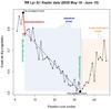 |
Fig. 2 Evolution of the light curve amplitude versus the pulsation cycle number during the first quarter of Kepler observations (Q1) conducted between 2009 May 16 and June 10. The strongest main shock occurs at the Blazhko maximum, the weakest at the Blazhko minimum. The sudden desynchronization of the photospheric layers occurs just after the strongest shock. A new synchronization of these layers would arise after a relaxation phase of the photosphere at the Blazhko minimum. The shock intensity would be amplified after the Blazhko minimum until the Blazhko maximum. These processes are not regular but they sometimes suffer high random fluctuations caused by physical processes of very different nature (shocks, gravitationnal infalling motion, radiative losses, etc.), occurring in the atmosphere. |
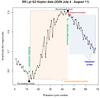 |
Fig. 3 Evolution of the light curve amplitude versus the pulsation cycle number during the second quarter of Kepler observations (Q2) conducted between 2009 July 4 and August 11. |
5.7. Shock amplification phase from Kepler data
We show the evolution of the light curve amplitude versus the pulsation cycle number during the first quarter of Kepler observations (Q1) conducted between 2009 May 16 and June 10 and during the second quarter of Kepler observations (Q2) conducted between 2009 July 4 and August 11, in Figs. 2 and 3.
Measuring the height of the rising branch of the light curve provides the light amplitude and consequently an estimate of the main shock intensity. Figure 3 gives the Kp amplitude of the light curve of RR Lyr during the second spacecraft roll (Q2) of the Kepler space telescope, between HJD 2 455 016 and HJD 2 455 054 (2009 July 4 and August 11). These light curves were published by Kolenberg et al. (2011) in their Fig. 4. The 68 consecutive pulsation cycles represent a time span of 39 days, equal to a Blazhko period. Between the minimum amplitude (cycle 12, Fig. 3) and the maximum amplitude (cycle 45), the shock intensity increases according to the process described above. The increase is not always regular and monotonous. From time to time, there is a gap (up to 0.1 Kp-magnitude) during the amplification phase of the shock (between cycles 22 and 35). In general, one gap is not immediately followed by a second gap. To achieve an amplification of the shock intensity, there are typically between two and four consecutive pulsation cycles. However, at each observed Blazhko cycle, the shock intensity increases until it reaches a maximum value. For RR Lyr, in both sets of observations Q1 and Q2 (Figs. 2, 3), the highest value corresponds to a maximum amplitude of about 0.9 Kp-magnitude. After this main shock of exceptional intensity, all subsequent shocks have a lower intensity, which, on average, continually decreases until the Blazhko minimum. We proposed above that the main shock intensity is amplified until it becomes high enough to cause the complete desynchronization of the photospheric layers. After this spectacular event, a relaxation phase occurs between the maximum and the Blazhko minimum. This is necessary to enable the re-synchronization of the layers.
Observations show that the pulsation of a non-Blazhko star is regular enough, with a good repetition of the light curves. Nevertheless, with four-shocks crossing the atmosphere at each pulsation cycle, a non-Blazhko star is not a perfect Swiss clock. With a sufficiently good level of accuracy, many small irregularities are observed from one pulsation cycle to another. Indeed, as already discussed above, shocks do not propagate in a homogeneous atmosphere, and several processes occur. First, the motion of the atmospheric layers is never perfectly synchronized. Thus, shocks can be accelerated or decelerated depending on atmospheric conditions and their rates of radiative losses. The four shocks, which pass through the whole atmosphere at each pulsation, merge among themselves at different phases and produce residual shocks of variable intensities. In addition, nonlinear interactions between shocks and atmospheric layers are complex and must increase with the amplitude of the pulsation. Despite all this, it may be noted that the pulsation of a non-Blazhko star remains relatively stable and steady.
The big difference in how a Blazhko star explains the strong irregularities observed is the presence of shock s3’. This shock slows down the infalling motion of the high atmospheric layers on the photosphere, causing a “collision” (a slowdown) with the infalling shock front s4+s3. The intensity of shock s3’ varies at each pulsation cycle due to radiative losses of the main shock, which are themselves variable from one cycle to another. Consequently, the nonlinear interaction between these two shock waves would cause irregularities and gaps such as observed in Blazhko stars (Figs. 2, 3).
Figure 2 gives the Kp-amplitude of the light curve of RR Lyr during the first roll (Q1), between HJD 2 454 967 and HJD 2 454 992 (2009 May 16th-June 10th). The original light curves are shown by Kolenberg et al. (2011) in their Fig. 4. The amplitude of the gap just after the shock of maximum intensity is variable. It is larger (0.1 Kp-magnitude) during Q1 than during Q2 (0.02 Kp-magnitude). In fact, it is rather when the intensity value of the main shock reaches a critical level that the desynchronization of photospheric layers occurs. For a given star, this value mainly depends on the gravity and, more incidentally, on physical conditions within the atmosphere.
Finally, the amplitude of the light curve of a Blazhko star, and accordingly the intensity of the main shock, follows a random path during the Blazhko cycle (Figs. 2, 3). This path strongly depends on the previous history of the dynamics of the atmosphere that occurred during the last pulsation cycle at the very least.
5.8. Amplitudes of Blazhko stars
Szeidl (1988) showed the amplitudes of non-modulated stars compared with those of Blazhko stars. The Blazhko effect introduces a dispersion of light curve amplitudes: the highest amplitude of Blazhko stars always fits the mean distribution of non-Blazhko stars, while the smallest ones induce a high dispersion at lower amplitudes. This author concluded that the Blazhko effect was a suppressing phenomenon that weakens the amplitude. As reported by Guggenberger (2013, priv. comm.), the behavior of some individual stars like V445 Lyr, where the amplitude almost disappears at the Blazhko minimum, seems to support this picture of a supressing Blazhko effect.
In our explanation of the Blazhko effect, this phenomenon is generated by desynchronization. During this phase, the pulsation of the atmosphere is completely destabilized. Thus, the amplitude of the pulsation can reach very low values as observed for V445 Lyr. When the pulsation of atmospheric layers are synchronized again, the amplification mechanism of the intensity of the main shock is activated. At the time of Blazhko maximum, the main shock reaches its greatest intensity.
Non-Blazhko stars may, like Blazhko stars, have very high amplitudes. The question is to know whether the maximum amplitude of Blazhko stars may be higher than that of non-Blazhko stars. If we consider the V-amplitude distribution of RR Lyr stars in M5 versus period (Jurcsik et al. 2011b), we see that the highest amplitudes are reached by Blazhko stars. Of course, because the number of stars used is too small, this result is not conclusive. Further studies need to be carried out to establish whether the amplification mechanism of the main shock is capable of producing shocks of higher intensity than in a regular pulsation like that of non-Blazhko stars.
5.9. Connection between pulsation and Blazhko periods
As shown by Jurcsik et al. (2005) from a sample of 894 Blazhko stars, the possible range of the Blazhko period depends on the pulsation period. Blazhko stars with a pulsation period shorter than 0.45 day can have a modulation period as short as a few days, whilst this cannot exceed about twenty days for a pulsation period longer than 0.625 day. In contrast, for the large majority of RRab stars in the range 0.45−0.625 day, Blazhko periods have a uniform distribution, without any correlation whatsoever between the two periods. However, these Blazhko periods are usually longer than 25 days. To explain the connection between the two periods at shorter and longer pulsation periods, Jurcsik et al. (2005) assumed that the Blazhko period corresponds to the rotational period of RR Lyrae stars. In this case, they showed that the distribution of the projected rotational velocities of red and blue horizontal branch stars at different effective temperatures shows a similar behavior as those derived for RR Lyr stars from their Blazhko periods. For pulsation periods shorter than 0.45 day, the number of RRab stars is too small to give a definitive finding about their distribution in this period range.
In our explanation of the Blazhko effect, the length of the Blazhko cycle is defined by the sum of the following two phases: (1) the duration of the amplification phase of the main shock intensity, which results in the desynchronization of the photospheric layers at Blazhko maximum and (2) the time used by the photosphere to regain its synchronous state occurring at Blazhko minimum. The duration of these phases depends on several factors, in particular, on the physical parameters of the star such as gravity. This probably explains why some stars sometimes deviate from the general distribution, even in the range 0.45−0.625 day.
The dispersion of Blazhko RRc stars is rather uniform, as can be seen in Figs. 4 and 6 of the Blazhko period distribution generated by Jurcsik et al. (2005). In previous sections, we reported that the shock intensity in RRc stars is expected to be three to four times weaker than in RRab stars. This means that, if the shock amplification mechanism is working, it is weak. Consequently, the duration of the relaxation phase of the photosphere may be short. This is why we can observe short Blazhko periods. However, depending on the value of the star parameters (mass, radius), long Blazhko periods may also be possible, as observed by Jurcsik et al. (2005).
5.10. Irregularities and period doublings
The explanation of the Blazhko effect that we have proposed above involves several independent factors. First, there are shock s3’ and the main shock, which reaches a high intensity. Next, during their infalling motion on the deep photosphere, atmospheric layers (which may be a time slowed down by s3’), are essentially governed by the gravitational force and the increasing compression on the deep photosphere. The shock amplitude depends on the physical conditions within the atmosphere and also on the rate of their radiative losses. The intensity of the κ-γ-mechanism depends on the intensity of the above mechanisms such as shocks. Finally, from one pulsation cycle to another, these physical processes are combined. From the point of view of energy, they are not independent because they influence each other in a nonlinear way. However, from Blazhko minimum to maximum, or during the reverse phase corresponding to the photospheric relaxation, the atmosphere evolves irreversibly because the average effective temperature changes the direction of variation twice during each Blazhko cycle. As a result, the various processes mentioned above cannot reach a state of equilibrium. Energy exchanges between all processes and their combinations are unstable and can therefore explain the more or less significant irregularities. Finally, the Blazhko effect would be like an energetic system with many degrees of freedom, constantly disturbed by the unstable radiative energy loss of the main shock. Under these conditions, it is not surprising that at any time of the Blazhko cycle and for an irregular time interval, a phenomenon similar to that of period doubling appears fortuitously for a time and then suddenly disappears. Finally, irregularities would be caused by a purely random process and not be the result of a chaotic system in the sense of a dynamical system.
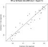 |
Fig. 4 First return map on the successive pair of the amplitude, n + 1 vs. n, during the second quarter of Kepler observations (Q2) conducted between 2009 July 4 and August 11. The first return map is shapeless, without particular structure, testifying to a rather random irregularity around the diagonal straight line, which is the identity map. |
Figure 4 shows the first-return map with the successive Kp-magnitude amplitude of the light curves during the Q2 set of Kepler observations (Fig. 3). We observe no particular form such as the triangular shape reported by Fokin (1994) for chaotic models of RV Tauri stars, or one and two-band chaotic cycles for models of W Virginis stars (Buchler & Kovacs 1987). Thus, we can propose that our shapeless first return map of RR Lyr is the consequence of a random irregularity. However, many more observations than those currently available to us are needed to confirm this trend.
Buchler & Kolláth (2011) used the amplitude equation formalism to study the 9:2 resonant interaction. They limited their amplitude equations to the coupling between the 9th overtone and the fundamental mode, although a resonance with any other higher mode is possible. Because the resulting amplitude equations have eleven free parameters, the authors imposed some constraints (for instance, they assumed to be inside the fundamental mode instability strip) to try to identify possible study solutions. Other remaining parameters were chosen arbitrarily to give a plausible stellar solution. In the solution presented, the temporal variation of the amplitude of the two modes show qualitative irregular modulations as observed in Blazhko stars. To determine the nature of these modulations, the authors constructed a first return map with the successive amplitude maxima of the light curves induced only by the fundamental mode. They showed the appearence of a well-defined structure called tent-like shape, indicating a chaotic origin due to the presence of a strange attractor. This theoretical approach is different from that based on observational curves because these are the sum of all excited pulsation modes. As a result, we cannot directly compare our first return map (Fig. 4) with that obtained by Buchler & Kolláth (2011). Is the tent-like structure still present if the theoretical light curves has been based on both considered modes? It would be interesting to know the answer to this question.
5.11. Connection with the pulsation mode switch?
As first suggested by van Albada & Baker (1973) and shown by Caputo et al. (1978), the evolution of the pulsation mode of a RR Lyrae star depends on its evolutionary history starting from the zero-age horizontal branch (ZAHB). In fact, if a star evolves from a ZAHB point bluer than the fundamental blue edge (FBE), then RRab pulsators (F-mode) can be produced only at one time during their redward traveling after the FBE (see their Fig. 3). The star evolves from a ZAHB point redder than the FBE, the star should change its pulsation mode twice: the first time during its blueward evolution at the FBE, and a second time at the first overtone red edge (FORE) during its redward evolution. In this case, we have first the mode switch: F-FO, and then FO-F. In fact, in the intermediate region located between the FBE and FORE edges, a region called the “either-or region” (or “hysteresis region”), both fundamental and first overtone show a stable limit cycle, and can therefore coexist. Thus, a redward traveling star (RRc-type) preserves its previous pulsation mode (FO), whereas a blueward traveling star (RRab-type) continues in the F-mode. This is a hysteresis phenomenon for RR Lyrae stars crossing the IS. Using a large-scale survey of nonlinear pulsations in the RR Lyrae IS, Szabó et al. (2004) also found that the pulsational state depends on the direction of the evolutionary tracks. In the course of their survey, these authors have also encounted another type of hysteresis, namely a very narrow region where either fundamental (RRab) or double-mode (RRd) are possible. This hysteresis occurs solely during redway evolution but the possibility that blueward or both blue- and redward evolution produce double-mode stars is not excluded. Thus, as RRd have approximately the same amplitude as RRc, the intensity of their shocks is probably similar. Therefore, it is possible that there are some RRd Blazhko stars but their number is certainly very small.
In a recent paper, Arellano Ferro et al. (2012) showed that Blazhko RRc and Blazhko RRab stars in the globular cluster M53 are on average redder than their non-modulated counterparts (see their Fig. 8). This observational result is based on the V − I color distribution of 18 RRab (with 10 Blazhko) and 22 RRc (with 18 Blazhko) stars. According to this, RRab and RRc Blazhko stars would be cooler than non-Blazhko stars. This is not consistent with the location of Blazhko RRab stars from the Galactic field in the HRD (see Fig. 1). Indeed, the location of non-Blazhko stars is redder and closer to the fundamental mode red-edge than that of Blazhko stars that are in the either-or region, i.e., between the FBE and FORE edges.
During their long-term photometric monitoring of the globular cluster M5, Jurcsik et al. (2011b) studied properties of a sample of 50 RRab stars in which 20 stars are identified as or suspected to be Blazhko stars. They showed that Blazhko stars have systematically larger amplitude, shorter period, and fainter mean V-magnitude than regular RR Lyrae stars. In addition to these specific features in the location of Blazhko stars, Jurcsik et al. (2011b) noted that the population of RR Lyrae in globular clusters is either rich in Blazhko stars or in RRd stars or in both, while the Blazhko effect is common among Galactic-field RRab stars, where RRd are rare. Thus, a possible connection between the Blazhko effect and the star evolution may be related to mode switching between the fundamental and the first overtone modes. Nemec (1985) previously noted a possible relation between Blazhko variables and RRd stars in the Draco dwarf galaxy. It is also suggested that irregular changes observed in the pulsation period of Blazhko stars may be related to mode instabilities at or near the transition region separating RRc and RRab pulsators in the HRD.
Arellano Ferro et al. (2012) supported the idea that Blazhko modulations in RRc stars are connected with the pulsation mode switch. The Blazhko effect would appear systematically in stars undergoing a change in their pulsation mode. In this case, and following the Caputo et al. (1978) analysis, Blazhko RRab stars should appear immediately after the passage of FORE into the pure fundamental mode region. Thus, Blazhko RRab stars should be only located in the region between FORE and FRE limits. This does not seem to be the case. Similarly, Blazhko RRc stars should be located in the region of the pure first overtone, just after passing the FBE limit. As the number of known Blazhko RRc stars is limited at present, it is currently difficult to clarify this point. Additional observations are necessary.
In the framework of our explanation of the Blazhko effect, the fact that the pulsation mode of a RR Lyrae star depends on its evolutionary history from the ZAHB and can change when the star passes through the FBE or FORE limits, does not determine its physical origin. Following Caputo et al. (1978), due to the hysteresis mechanism, RRc or RRab stars change or do not change their pulsation mode when they cross FBE or FORE. Thus, it is not the mode switch that triggers or stops the Blazhko effect. Indeed, in our explanation, it is only the presence or absence of shock s3’ that determines the appearance of the Blazhko effect. In other words, the star may be within the intermediate region of the IS in which stable pulsations both in the first overtone mode or in the fundamental are possible. Thus, the Blazhko effect does not always manifest in stars undergoing a pulsation mode switch when they penetrate the either-or region. Indeed, when an RRab comes from the pure fundamental region of the IS (redward traveling), the star becomes a Blazhko star but continues to pulsate in the fundamental mode in the either-or region. We have the same situation when an RRc from the purely first overtone mode region penetrates the either-or region. Arellano Ferro et al. (2012), using the fact that the distribution of the Blazhko RRc variables is redder than that of the non-modulated RRc in the globular cluster M53, proposed that the Blazhko effect manifests systematically in stars undergoing a change in pulsation mode. This statement does not seem consistent with our explanation of the Blazhko effect.
6. Conclusion
We proposed a new explanation of the Blazhko effect. The mechanism is based on the role played by two shock waves in connection with the dynamics of atmospheric layers, especially photospheric layers. We assumed that two pulsation modes are systematicaly excited in Blazhko stars in contrast to non-Blazhko stars. In addition to the fundamental mode, which almost reached its limit cycle, the first overtone is marginally excited. Shock s3’ recorded by Fokin & Gillet (1997) may be generated by the perturbation of the fundamental mode by the transient first overtone. Molnár et al. (2012a) reported, for the first time, the detection of the first overtone in the Kepler observations of RR Lyr, but with a very weak amplitude level. Of course, the fundamental mode plays a dominant role in RRab, while the situation is reversed in RRc when the star moves into the either-or region of the IS.
There is a damping effect during the infalling motion of atmospheric layers on the photosphere. This deceleration is particularly marked when s3’ merges with the infalling shock front s4+s3. This sudden deceleration, somewhat like a collision, produces a decrease in atmospheric compression that in turn affects the κ-mechanism. The second shock, called the main shock, has the highest intensity among the five shocks propagating in the atmosphere at each pulsation cycle (Fokin & Gillet 1997). The Mach number of the main shock can be large (M > 15). In these conditions, Fadeyev & Gillet (2001) have shown that most of the kinetic energy of the shock is lost as radiation (>70%). This effect should cause a small decrease (about 1%) of the average effective temperature between the Blazhko minimum and maximum.
By definition, non-Blazhko stars do not present modulations. The dynamics of their atmosphere is only perturbed by four shocks during each pulsation cycle, as in classical Cepheids (Fokin et al. 1996). Indeed, shock s3’ is not present because the first overtone is not excited. Consequently, there is no sudden dampening effect during the free fall motion of the atmosphere. Observations show that the light curves of non-Blazhko stars are reproducible with a good degree of accuracy. Nevertheless, this reproduction is not perfect and small departures are visible when data are analyzed in more detail. In Blazhko stars, shock s3’ is active. Its action completely destabilizes the dynamics of the atmosphere as far as generating a random behavior (modulations), which is not present in non-Blazhko stars.
The Blazhko effect can be described by two main steps. The first takes place from the Blazhko minimum to the maximum. During this interval, the main shock intensity is amplified. This amplification is not monotonous. Indeed, sometimes it undergoes random fluctuations of large amplitude but the average amplification is maintained. The second phase occurs from the Blazhko maximum to the minimum. At the Blazhko maximum, the intensity of the main shock reaches its highest value. For this value, the shock energy should be sufficient to completely desynchronized photospheric layers. This phenomenon provokes a sharp break of the amplification mechanism. This break can be also observed through the change of direction of variation of the pulsational parameters such as the pulsation period or the amplitude of the light curve. From this moment, the average effective temperature increases. The motion of photospheric layers being destabilized, a relaxation phase takes place until the Blazhko minimum is reached. At this point, the photosphere becomes re-synchronized.
In our explanation of the Blazhko effect, it is possible to understand the phenomenon of helium occurrence. It is directly connected with the amplification mechanism occurring in Blazhko stars. At the Blazhko maximum, the main shock reaches its highest intensity while it is lowest at the Blazhko minimum. Thus, it is normal that helium emission lines are only observed around the Blazhko maximum and only in stars in which the intensity of the main shock is high enough to excite helium. He II emission may only be detected in Blazhko stars with shocks of exceptional intensity.
Because the Blazhko effect, induced by atmospheric shocks, shows the behavior of a purely random process, it is possible to understand the “PD effect” recently observed in a few Blazhko stars in the Kepler data and why this is a transient and unpredictable phenomenon. Thus, it would not be necessary to involve a classical chaotic system, in the sense of dynamical systems such as proposed by Buchler & Kolláth (2011), to explain the Blazhko effect. Many interesting features, such as the first and the ninth overtones, during cycle-to-cycle variations of RR Lyr were recently highlighted by Molnár et al. (2012a,b). It is possible that these features together with the interacting shock hypothesis proposed in this paper can explain the Blazhko effect. Indeed, if complex atmospheric motions induced by the different shocks propagating into the atmosphere have an erratic behavior, they may be the cause of the small observational features detected by these authors. More investigations in this area are necessary to clarify this supposition.
Because the Blazhko effect takes place in stars that are affected by the fundamental mode and the first overtone, it may also be observed in a part of RRc stars. Since 1999, observations have proven that the Blazhko effect is also a common effect (~50%) among RRc variables. Of course, the amplitude of shocks in RRc, especially the main one, is weaker than in RRab. If shock s3’ is not present in RRc, the physical mechanism causing the Blazhko effect in these stars is perharps not exactly the same that in RRab. In fact, to cause the Blazhko effect, it is sufficient that a shock wave disrupts the precarious balance between the main shock and the infalling motion of atmospheric layers in the photosphere. If the fundamental mode dominates, s3’ plays this role, while if the first overtone dominates, the disturbance of the fundamental mode on the first overtone must induce a shock equivalent to s3’. A theoretical approach is needed to identify the exact mechanism. High-resolution spectroscopic observations of RRc stars are required to achieve a complete observational investigation of the Blazhko effect in RRc stars. A similar investigation would be also useful for RRd stars although the Blazhko effect has not yet been detected in these rare stars.
Finally, the pulsation mode switch between the fundamental and the first overtone mode does not seem to be the cause of the Blazhko effect. According to our explanation of the Blazhko effect, when the star (an RRc or an RRab) penetrates the either-or region of the IS, the star becomes a Blazhko variable.
Acknowledgments
I wish to thank Agnès Lèbre and Philippe Mathias for helpful comments and valuable discussions that helped to improve the clarity of the paper. I want to thank Andrei Fokin for sending me the results of his RRc pulsation models before publication and his continued support during our ongoing collaboration. A big thank you to Elisabeth Guggenberger and Katrien Kolenberg for their relevant remarks and interesting suggestions. I am grateful to the anonymous referee for his/her very thoughtful reports that led to an improvement the text. I gratefully acknowledge Joanne O’Donnell and Astrid Peter for their very careful reading of the final version of this paper.
References
- Arellano Ferro, A., Bramich, D. M., & Figuera Jaimes, R., et al. 2012, MNRAS, 420, 1333 [NASA ADS] [CrossRef] [Google Scholar]
- Bailey, S. I. 1902, Harv. Coll. Observ. Annals, 38, 1 [Google Scholar]
- Benkö, J. M., Kolenberg, K., Szabó, R., et al. 2010, MNRAS, 409, 1585 [NASA ADS] [CrossRef] [Google Scholar]
- Blazhko, S. 1907, Astron. Nachr., 175, 325 [NASA ADS] [CrossRef] [Google Scholar]
- Buchler, J. R., & Goupil, M.-J. 1984, ApJ, 279, 394 [NASA ADS] [CrossRef] [MathSciNet] [Google Scholar]
- Buchler, J. R., & Kolláth, Z. 2011, ApJ, 731, 24 [NASA ADS] [CrossRef] [Google Scholar]
- Buchler, J. R., & Kovacs, G. 1987, ApJ, 320, L57 [NASA ADS] [CrossRef] [MathSciNet] [Google Scholar]
- Burki, G. A., & Meylan, G. 2001, A&A, 156, 131 [NASA ADS] [Google Scholar]
- Caputo, F., Castellani, V., & Tornambe, A. 1978, A&A, 67, 107 [NASA ADS] [Google Scholar]
- Dorman, B. 1992, ApJS, 81, 221 [NASA ADS] [CrossRef] [Google Scholar]
- Fadeyev, Yu. A., & Gillet, D. 1998, A&A, 333, 687 [NASA ADS] [Google Scholar]
- Fadeyev, Yu. A., & Gillet, D. 2001, A&A, 368, 901 [NASA ADS] [CrossRef] [EDP Sciences] [Google Scholar]
- Fokin, A. B. 1994 A&A, 292, 133 [Google Scholar]
- Fokin, A. B., & Gillet, D. 1994, A&A, 290, 875 [NASA ADS] [Google Scholar]
- Fokin, A. B., & Gillet, D. 1997, A&A, 325, 1013 [NASA ADS] [Google Scholar]
- Fokin, A. B., Gillet, D., & Breitfellner, M. G. 1996, A&A, 307, 503 [NASA ADS] [Google Scholar]
- Fokin, A. B., Gillet, D., & Chadid, M. 1999, A&A, 344, 930 [NASA ADS] [Google Scholar]
- Fokin, A. B., Massacrier, G., & Gillet, D. 2000, A&A, 355, 668 [NASA ADS] [Google Scholar]
- Fokin, A. B., Massacrier, G., & Gillet, D. 2004, A&A, 420, 1047 [NASA ADS] [CrossRef] [EDP Sciences] [Google Scholar]
- Gillet, D., & Crowe, R. A. 1988, A&A, 199, 242 [NASA ADS] [Google Scholar]
- Gillet, D., Burki, G., & Crowe, R. A. 1989, A&A, 225, 445 [Google Scholar]
- Gillet, D., Debiève, J.-F., Fokin, A. B., et al. 1998, A&A, 332, 235 [NASA ADS] [Google Scholar]
- Gillet, D., Fokin, A. B., Breitfellner, M. G., et al. 1999, A&A, 344, 935 [NASA ADS] [Google Scholar]
- Gillet, D., Fabas, N., & Lèbre, A. 2013, A&A, 553, A59 [NASA ADS] [CrossRef] [EDP Sciences] [Google Scholar]
- Guggenberger, E., & Kolenberg, K. 2006, Comm. Asteroseismology, 148, 21 [NASA ADS] [CrossRef] [Google Scholar]
- Guggenberger, E., & Kolenberg, K. 2007, Comm. Asteroseismology, 150, 379 [NASA ADS] [CrossRef] [Google Scholar]
- Guggenberger, E., Kolenberg, K., Chapellier, E., et al. 2011, MNRAS, 415, 1577 [NASA ADS] [CrossRef] [Google Scholar]
- Guggenberger, E., Kolenberg, K., Nemec, J. M., et al. 2012, MNRAS, 424, 649 [NASA ADS] [CrossRef] [Google Scholar]
- Hardie, R. H. 1955, ApJ, 122, 256 [NASA ADS] [CrossRef] [Google Scholar]
- Hill, S. J. 1972, ApJ, 178, 793 [NASA ADS] [CrossRef] [Google Scholar]
- Jurcsik, J., Szeidl, B., Nagy, A., & Sodor, A. 2005, Acta Astron., 55, 303 [Google Scholar]
- Jurcsik, J., Szeidl, B., Sodor, A., et al. 2006, AJ, 132, 61 [NASA ADS] [CrossRef] [Google Scholar]
- Jurcsik, J., Sodor, A., Szeidl, B., et al. 2009a, MNRAS, 393, 1553 [NASA ADS] [CrossRef] [Google Scholar]
- Jurcsik, J., Hurta, Zs., Sodor, A., et al. 2009b, MNRAS, 397, 350 [NASA ADS] [CrossRef] [Google Scholar]
- Jurcsik, J., Sodor, A., Szeidl, B., et al. 2011a, MNRAS, 411, 1585 [NASA ADS] [CrossRef] [Google Scholar]
- Jurcsik, J., Szeidl, B., Clement, C., et al. 2011b, MNRAS, 411, 1763 [NASA ADS] [CrossRef] [Google Scholar]
- Jurcsik, J., Sodor, A., Hajdu, G., et al. 2012, MNRAS, 423, 993 [NASA ADS] [CrossRef] [Google Scholar]
- Kluyver, H. A. 1936, BAN, 7, 313 [NASA ADS] [Google Scholar]
- Kolenberg, K. 2012, JAAVSO, 40, 481 [Google Scholar]
- Kolenberg, K., & Bagnulo, S. 2009, A&A, 498, 543 [NASA ADS] [CrossRef] [EDP Sciences] [Google Scholar]
- Kolenberg, K., Smith, H. A., Gazeas, K. D., et al. 2006, A&A, 459, 577 [Google Scholar]
- Kolenberg, K., Bryson, S., & Szabó, R. 2011, MNRAS, 411, 878 [NASA ADS] [CrossRef] [Google Scholar]
- Kolláth, Z., Molnár, L., & Szabó, R. 2011, MNRAS, 414, 1111 [NASA ADS] [CrossRef] [Google Scholar]
- Le Borgne, J.-F., & Klotz, A. 2009, GEOS Note Circulaire NC, 1105 [Google Scholar]
- Mihalas, D., & Mihalas, B. W. 1984, Foundations of Radiation Hydrodynamics (New York: Oxford University Press, Paperback Edition) [Google Scholar]
- Molnár, L., Kollaťh, Z., Szabó, R., et al. 2012a, ApJ, 757, L13 [Google Scholar]
- Molnár, L., Kollaťh, Z., Szabó, R., et al. 2012b, Astron. Nachr., 333, 950 [NASA ADS] [Google Scholar]
- Nemec, J. M. 1985, AJ, 90, 204 [NASA ADS] [CrossRef] [Google Scholar]
- Nemec, J. M., Smolec, R., Benkö, J. M., et al. 2011, MNRAS, 417, 1022 [NASA ADS] [CrossRef] [Google Scholar]
- Olech, A., Kaluzny, J., Thompson, I. B., et al. 1999, AJ, 118, 442 [NASA ADS] [CrossRef] [Google Scholar]
- Poretti, E., Paparo, M., Deleuil, M., et al. 2010, A&A, 520, A108 [NASA ADS] [CrossRef] [EDP Sciences] [Google Scholar]
- Prager, R. 1916, Sitzb. Ak. Berlin, 8, 216 [Google Scholar]
- Preston, G. W. 1964, ARA&A, 2, 23 [NASA ADS] [CrossRef] [Google Scholar]
- Preston, G. W. 2009, A&A, 507, 1621 [NASA ADS] [CrossRef] [EDP Sciences] [Google Scholar]
- Preston, G. W. 2011, AJ, 141, 6 [NASA ADS] [CrossRef] [Google Scholar]
- Pietrynski, G., Thompson, I. B., Gieren, W., et al. 2010, Nature, 468, 542 [NASA ADS] [CrossRef] [PubMed] [Google Scholar]
- Shapley, H. 1916, ApJ, 43, 217 [NASA ADS] [CrossRef] [Google Scholar]
- Skarka, M. 2013, A&A, 549, A101 [NASA ADS] [CrossRef] [EDP Sciences] [Google Scholar]
- Smolec, R., & Moskalik, P. 2008, Acta Astron., 58, 193 [NASA ADS] [Google Scholar]
- Smolec, R., Moskalik, P., Kolenberg, K., et al. 2011, MNRAS, 414, 2950 [NASA ADS] [CrossRef] [Google Scholar]
- Sodor, A. 2009, Stellar Pulsation: Challenges for Theory and Observations, eds. J. A. Guzik, & P. Bradley, Proc. AIP, 1170, 294, [Google Scholar]
- Sodor, A., Jurcsik, J., & Szeidl, B. 2009, MNRAS, 394, 261 [NASA ADS] [CrossRef] [Google Scholar]
- Sodor, A., Jurcsik, J., & Szeidl, B. 2011, MNRAS, 411, 1585 [NASA ADS] [CrossRef] [Google Scholar]
- Sodor, A., Hajdu, G., Jurcsik, J., et al. 2012, MNRAS, in press [Google Scholar]
- Soszyński, I., Udalski, A., Szymański, M. K., et al. 2003, Acta Astron., 53, 93 [NASA ADS] [Google Scholar]
- Soszyński, I., Udalski, A., Szymański, M. K., et al. 2009, Acta Astron., 59, 1 [NASA ADS] [Google Scholar]
- Soszyński, I., Dziembowski, W. A., Udalski, A., et al. 2011, Acta Astron., 61, 1 [NASA ADS] [Google Scholar]
- Stellingwerf, R. F. 1975, ApJ, 199, 705 [NASA ADS] [CrossRef] [Google Scholar]
- Stothers, R. B. 2006, ApJ, 652, 643 [NASA ADS] [CrossRef] [Google Scholar]
- Stothers, R. B. 2010, PASP, 122, 536 [NASA ADS] [CrossRef] [Google Scholar]
- Struve, O., & Blaauw, A. 1948, ApJ, 108, 60 [NASA ADS] [CrossRef] [Google Scholar]
- Szabó, R., Kolláth, Z., & Buchler, J. R. 2004, A&A, 425, 627 [NASA ADS] [CrossRef] [EDP Sciences] [Google Scholar]
- Szabó, R., Kolláth, Z., Molnár, L., et al. 2010, MNRAS, 409, 1244 [NASA ADS] [CrossRef] [Google Scholar]
- Szczygiel, D. M., & Fabrycky, D. C. 2007, MNRAS, 377, 1263 [NASA ADS] [CrossRef] [Google Scholar]
- Szeidl, B. 1976, Multimode Periodic Variable Stars, Proc. IAU Colloq. 29, held in Budapest, September 1−5, 1975, ed. W. S. Fitch (D. Reidel Publishers), 133 [Google Scholar]
- Szeidl, B. 1988, Multimode Stellar Pulsations, Proc. of the Workshop, held in Budapest, September 1−3, 1987, eds. G. Kovacs, L. Szabados, & B. Szeidl (Budapest: Konkoly Observatory, Kultura), 45 [Google Scholar]
- van Albada, T. S., & Baker, N. 1973, ApJ, 185, 447 [Google Scholar]
All Tables
All Figures
|
Fig. 1 HR diagram adapted from Nemec et al. (2011) showing the locations of the Kepler non-Blazhko RR Lyrae stars (squares) compared with the Blazhko stars (circles) with known luminosity and effective temperature (see Table 1). For non-Blazhko stars, the luminosity was derived from stellar pulsation models, which take into account mass loss in contrast to evolution models. The blue and red edges for the IS were computed using the Warsaw pulsation code. The fundamental mode edges (FBE, FRE) are plotted as solid lines, and first overtone mode edges (FOBE, FORE) as dashed lines. The two sets of HB models (low- and high-metallicity) are taken from Dorman (1992). The numbers on the evolutionary tracks give the masses of evolution models. |
| In the text | |
|
Fig. 2 Evolution of the light curve amplitude versus the pulsation cycle number during the first quarter of Kepler observations (Q1) conducted between 2009 May 16 and June 10. The strongest main shock occurs at the Blazhko maximum, the weakest at the Blazhko minimum. The sudden desynchronization of the photospheric layers occurs just after the strongest shock. A new synchronization of these layers would arise after a relaxation phase of the photosphere at the Blazhko minimum. The shock intensity would be amplified after the Blazhko minimum until the Blazhko maximum. These processes are not regular but they sometimes suffer high random fluctuations caused by physical processes of very different nature (shocks, gravitationnal infalling motion, radiative losses, etc.), occurring in the atmosphere. |
| In the text | |
|
Fig. 3 Evolution of the light curve amplitude versus the pulsation cycle number during the second quarter of Kepler observations (Q2) conducted between 2009 July 4 and August 11. |
| In the text | |
|
Fig. 4 First return map on the successive pair of the amplitude, n + 1 vs. n, during the second quarter of Kepler observations (Q2) conducted between 2009 July 4 and August 11. The first return map is shapeless, without particular structure, testifying to a rather random irregularity around the diagonal straight line, which is the identity map. |
| In the text | |
Current usage metrics show cumulative count of Article Views (full-text article views including HTML views, PDF and ePub downloads, according to the available data) and Abstracts Views on Vision4Press platform.
Data correspond to usage on the plateform after 2015. The current usage metrics is available 48-96 hours after online publication and is updated daily on week days.
Initial download of the metrics may take a while.