| Issue |
A&A
Volume 553, May 2013
|
|
|---|---|---|
| Article Number | A100 | |
| Number of page(s) | 9 | |
| Section | The Sun | |
| DOI | https://doi.org/10.1051/0004-6361/201220319 | |
| Published online | 16 May 2013 | |
Radial profile of the inner heliospheric magnetic field as deduced from Faraday rotation observations
1
INAF – Osservatorio Astrofisico di Torino, Strada Osservatorio 20, 10025
Pino Torinese,
Italy
e-mail: This email address is being protected from spambots. You need JavaScript enabled to view it.
2
Laboratory for Astroparticle Physics, University of Nova
Gorica, 5000
Nova Gorica,
Slovenia
Received:
31
August
2012
Accepted:
27
March
2013
Abstract
Faraday rotation measures (RMs) of the polarized emission from extragalactic radio sources occulted by the coronal plasma were used to infer the radial profile of the inner heliospheric magnetic field near the solar minimum. By inverting LASCO/SOHO polarized brightness (pB) data taken during the observations in May 1997, we retrieved the electron density distribution along the lines of sight to the sources, which allowed us to separate the two plasma properties that contribute to the observed RMs. By comparing the observed RM values with those theoretically predicted by a power law model of the radial component of the coronal magnetic field using a best-fitting procedure, we found that the radial component of the inner heliospheric magnetic field can be nicely approximated by a power law of the form Br = 3.76 r-2.29 G in a range of heights from about 5 to 14 R⊙. Finally, our analysis suggests that the radial computation of the potential field source surface model from the Wilcox Solar Observatory is the preferred choice near solar minimum assuming a radial field in the photosphere and a source surface located at Rss = 2.5 R⊙.
Key words: Sun: corona / Sun: magnetic topology / Sun: radio radiation
© ESO, 2013
1. Introduction
Despite its fundamental importance, no direct information is available as yet on the inner heliospheric magnetic field; the innermost in situ measurements are still those obtained in the seventies by the two Helios probes at ~62 R⊙. Such crucial measurements in the region where the solar wind is heated, accelerated and decoupled from the coronal plasma, will only be available with the advent of the Solar Probe Plus mission1, planned by NASA to be launched no later than 2018. On the final three orbits, Solar Probe Plus will be able to fly within 8.5 R⊙ from the Sun’s surface. Empirical estimates of magnetic fields in the inner heliosphere are only possible very close to the base of the corona (e.g., Lin et al. 2000; Lee 2007), but their outward extrapolation often involves simplistic potential (or force-free) assumptions and the hypothesis of low plasma β, which may not be appropriate in the outer corona (Gary 2001). Under appropriate assumptions, magnetic field strength estimates in the outer corona have been obtained from the analysis of the radiation emitted during the passage of coronal shock waves (e.g., Mancuso et al. 2003; Vršnak et al. 2004; Cho et al. 2007; Bemporad & Mancuso 2010; Gopalswamy & Yashiro 2011; Kim et al. 2012). However, one of the best observational methods for obtaining information on the strength and radial profile of the magnetic field in the inner heliosphere still remains the analysis of Faraday rotation measurements of linearly polarized radio signals from galactic or extragalactic radio sources (e.g., Sakurai & Spangler 1994; Mancuso & Spangler 1999, 2000; Spangler 2005; Ingleby et al. 2007; Mancuso & Garzelli 2007; Ord et al. 2007) or from the transmitter of a spacecraft (e.g., Stelzried et al. 1970; Pätzold et al. 1987; Jensen et al. 2005). For a fairly recent comprehensive review of coronal Faraday rotation observations, see Bird (2007).
To understand the physics behind the Faraday effect, it is useful to consider a linearly
polarized wave as two counter-rotating circularly polarized waves. Faraday rotation occurs
because the phase velocity of the left circularly polarized component travels faster along
the magnetic field than the right circularly polarized component, which results in a net
rotation Δξ of the wave’s polarization position angle given (in radians) by
 (1)In this equation, expressed in cgs units,
λ is the wavelength of the radio signal, ne
is the electron density, B is the vector magnetic field,
ds is the vector incremental path defined to be positive
toward the observer, e and me are the charge
and mass of the electron, and c is the speed of light. The expression can
also be written as Δξ = λ2RM,
where RM is the rotation measure (RM), defined to be positive if
B is pointed toward the observer. Essentially, RM yields
information on the integrated product of the line of sight (LOS) component of the magnetic
field and the electron density. Since Faraday rotation is an integrated quantity and
proportional to the product of two independent quantities, in order for the magnetic field
component of the observed RM to be determined, there must be an independent determination of
the electron density, whether from observations or models. For a spherically symmetric
corona, that is, with a perfectly symmetric electron density and magnetic field
distribution, the obvious result would be RM ≈ 0 at all latitudes. This is
because the LOS component of the magnetic field would reverse at the point of closest
approach to the Sun. Overall, the analysis of the Faraday rotation observations reduced by
Mancuso & Spangler (2000) showed values different
from zero, reaching a highest value (in absolute magnitude) of −10.6 rad m-2 for
one of the radio sources at ~6 R⊙. According to this
study, this effect was mostly attributed to an asymmetric distribution of the electron
density along the LOS, thus working as a “weighting function” for an otherwise symmetric
magnetic field distribution. Although the electron density distribution used in Mancuso
& Spangler (2000) was not symmetric, it was still
an analytical approximation inspired by the work of Guhathakurta et al. (1996), with two different analytical expressions for the
streamer and coronal hole components. Because of this assumption, no attempt was made to
derive an analytical expression for the radial component of the magnetic field with a
best-fitting procedure. Moreover, in that work, the position of the magnetic neutral line,
which coincides with the heliospheric current sheet, was deduced from a potential field
expansion of the photospheric magnetic data from the Wilcox Solar Observatory (WSO) and
using a potential field source surface (PFSS) model (Altschuler & Newkirk 1969; Schatten et al. 1969) with a source surface at a fixed height of
2.5 R⊙. Although Mancuso & Spangler (2000) were able to obtain a fair agreement between RM model and
observations, their analysis was only able to support the validity of the Pätzold et al.
(1987) coronal magnetic field model, which was used
in input as an approximate expression for the radial magnetic field profile at the heights
covered by the RM observations.
(1)In this equation, expressed in cgs units,
λ is the wavelength of the radio signal, ne
is the electron density, B is the vector magnetic field,
ds is the vector incremental path defined to be positive
toward the observer, e and me are the charge
and mass of the electron, and c is the speed of light. The expression can
also be written as Δξ = λ2RM,
where RM is the rotation measure (RM), defined to be positive if
B is pointed toward the observer. Essentially, RM yields
information on the integrated product of the line of sight (LOS) component of the magnetic
field and the electron density. Since Faraday rotation is an integrated quantity and
proportional to the product of two independent quantities, in order for the magnetic field
component of the observed RM to be determined, there must be an independent determination of
the electron density, whether from observations or models. For a spherically symmetric
corona, that is, with a perfectly symmetric electron density and magnetic field
distribution, the obvious result would be RM ≈ 0 at all latitudes. This is
because the LOS component of the magnetic field would reverse at the point of closest
approach to the Sun. Overall, the analysis of the Faraday rotation observations reduced by
Mancuso & Spangler (2000) showed values different
from zero, reaching a highest value (in absolute magnitude) of −10.6 rad m-2 for
one of the radio sources at ~6 R⊙. According to this
study, this effect was mostly attributed to an asymmetric distribution of the electron
density along the LOS, thus working as a “weighting function” for an otherwise symmetric
magnetic field distribution. Although the electron density distribution used in Mancuso
& Spangler (2000) was not symmetric, it was still
an analytical approximation inspired by the work of Guhathakurta et al. (1996), with two different analytical expressions for the
streamer and coronal hole components. Because of this assumption, no attempt was made to
derive an analytical expression for the radial component of the magnetic field with a
best-fitting procedure. Moreover, in that work, the position of the magnetic neutral line,
which coincides with the heliospheric current sheet, was deduced from a potential field
expansion of the photospheric magnetic data from the Wilcox Solar Observatory (WSO) and
using a potential field source surface (PFSS) model (Altschuler & Newkirk 1969; Schatten et al. 1969) with a source surface at a fixed height of
2.5 R⊙. Although Mancuso & Spangler (2000) were able to obtain a fair agreement between RM model and
observations, their analysis was only able to support the validity of the Pätzold et al.
(1987) coronal magnetic field model, which was used
in input as an approximate expression for the radial magnetic field profile at the heights
covered by the RM observations.
The aim of this work is to improve the previous analysis of Mancuso & Spangler (2000) by introducing direct information on the electron density distribution along the LOS for the above observations, thus allowing to obtain an estimate of the strength and radial profile of the inner heliospheric magnetic field. In this work, instead of using an analytical model for the electron density distribution along the LOS, we obtain this quantity empirically through inversion of polarized brightness (pB) measurements obtained from observations of the Large Angle and Spectrometric COronagraph (LASCO; Brueckner et al. 1995) telescope onboard the Solar and Heliospheric Observatory (SOHO; Domingo et al. 1995) spacecraft during the same days as the observations of the radio sources. In this way, we will be able to infer with a best-fitting procedure the radial profile of the magnetic field of the inner heliosphere that best accounts for the observed RMs. As a by-product of our study, we will also be able to evaluate the most suitable PFSS model among the three models available from the WSO.
This paper is organized as follows. In Sect. 2, we present some details of the observations and of the data reduction procedure. In Sect. 3, we introduce the magnetic field model. In Sect. 4, we compare the model with observations and discuss our results. Finally, a summary and conclusions are given in Sect. 5.
 |
Fig. 1 Location of the radio sources relative to the Sun on each of the four days of observation. The bull’s eye symbol indicates the position of the Sun and the dotted line is the ecliptic. The size of the plotted symbol is a rough indicator of the absolute magnitude of the RM. Red squares correspond to positive RMs and blue circles represent negative RMs. |
2. Observations and data reduction
2.1. Radio observations
The observations of the radio sources discussed in this paper were made on four days in 1997 (May 6, 11, 22, and 26) with the Very Large Array (VLA) radio telescope of the National Radio Astronomy Observatory (NRAO). Each source was reobserved far from the Sun at the same frequencies to obtain the intrinsic RM and that from the interstellar medium but without a coronal contribution. The frequencies used were 1465 MHz with a bandwidth of 50 MHz and 1665 MHz with a bandwidth of 25 MHz and were chosen to have sufficient separation in λ2 to allow for an accurate determination of the RMs. Ionospheric calibration was carried out to correct for ionospheric Faraday rotation. Two major factors limiting the accuracy of VLA polarization measurements are the removal of ionospheric Faraday rotation and the correction for instrumental polarization. The task FARAD of the NRAO Astronomical Image Processing System (AIPS) was used for ionospheric RM estimation and correction. This task calculates the appropriate Faraday rotation correction using a phenomenological model of the ionospheric electron density. This model (Chiu 1975) takes as input the monthly average Zurich sunspot number to estimate the ionospheric electron column density. The adequacy of the ionospheric correction was tested by observing four sources far from the Sun, where coronal Faraday rotation is negligible. For these sources the standard deviation of the rotation measure fluctuations around the mean was about 0.3 rad m-2 (see Mancuso & Spangler 2000, for details). This quantity can be considered as a rough estimate of the measurement errors introduced by residual ionospheric Faraday rotation or instrumental polarization errors. In both coronal and reference observations, the instrumental polarization (and subsequent correction) was calibrated by observing a calibrator source over a broad range in parallactic angle. The procedure used is described in Mancuso & Spangler (1999). The observations of the radio sources discussed in this paper sampled solar elongations from ~5 to 14 R⊙ at various heliographic latitudes through 13 different lines of sight (see Fig. 1), with values for the RMs ranging from −10.6 to + 3.3 rad m-2. More specific information on the VLA observations used for this work and on the data reduction can be found in Mancuso & Spangler (2000) and is not repeated here.
2.2. White-light observations
Observations of the extended corona are primarily obtained with white-light coronagraphs
that are able to observe coronal structures that are highlighted by the photospheric
radiation Thomson-scattered by electrons in the ionized coronal plasma. The observable
polarized brightness (pB) is defined as the difference in intensity of
radiation that is polarized tangential to the limb of the Sun and radiation that is
polarized normal to the limb. This quantity is directly related to the coronal electron
density by  (2)where ne is the
electron density, T(r) is the Thomson-scattering
function, and the integral is carried out along the LOS. In general, it is difficult to
infer the density distribution in the corona and inner heliosphere from remote-sensing
techniques since the signals usually derive from the contribution of a superposition of
different structures integrated along the LOS in the optically thin intervening plasma.
Coronal mass ejections can also drastically affect the pB data as well as
disturb the overall structure of the corona in a temporal scale of a few hours.
Notwithstanding the above observational caveats, transient phenomena are much less common
during solar minimum conditions. Moreover, the overall structure of the corona is observed
to be axially symmetric by a high degree during the periods with lower solar activity due
to the dominance of the dipolar component of the global magnetic field of the Sun. The
electron density distribution can thus be estimated with a good degree of confidence from
the observed pB using a technique developed by Van de Hulst (1950) that is particularly appropriate in the
near-symmetric density distribution observed during solar minima conditions (e.g., Gibson
et al. 1999). In this work, the
pB data, recorded daily around the Sun by the LASCO C2 telescope that
observes the solar corona between about 2 and 6 R⊙, were
inverted by fitting the observed radial profiles at steps of 3° of heliographic latitude.
These pB radial profiles were then inverted with the above mentioned
technique to yield electron density radial profiles below about
6 R⊙. Finally, radial power fits of the form
ne(r) = Ar−α + Br-2
were performed to extend the profiles to 1 AU. Once the electron density maps were
produced, the data were placed in a rectangular grid with observation times converted to
Carrington longitudes, and the Carrington maps were finally resampled by using a moving
smooth filter and then a moving average, both applied to all pixels. In addition to
assuming that the corona is essentially stationary during the period corresponding to our
observations, the above reconstruction of the global coronal electron density implicitly
assumes that the observed Thomson-scattered radiation is dominated by a relatively thin
layer of scattering electrons centered on the point of closest approach to the Sun. This
is clearly a zero-order approximation, since the actual pB should be
considered as a weighted sum of contributions to the Thomson-scattered radiation from
electrons along the entire LOS. However, it is a fairly safe assumption given that the
electron density distribution in the corona falls off with distance as a high-exponent
power-law.
(2)where ne is the
electron density, T(r) is the Thomson-scattering
function, and the integral is carried out along the LOS. In general, it is difficult to
infer the density distribution in the corona and inner heliosphere from remote-sensing
techniques since the signals usually derive from the contribution of a superposition of
different structures integrated along the LOS in the optically thin intervening plasma.
Coronal mass ejections can also drastically affect the pB data as well as
disturb the overall structure of the corona in a temporal scale of a few hours.
Notwithstanding the above observational caveats, transient phenomena are much less common
during solar minimum conditions. Moreover, the overall structure of the corona is observed
to be axially symmetric by a high degree during the periods with lower solar activity due
to the dominance of the dipolar component of the global magnetic field of the Sun. The
electron density distribution can thus be estimated with a good degree of confidence from
the observed pB using a technique developed by Van de Hulst (1950) that is particularly appropriate in the
near-symmetric density distribution observed during solar minima conditions (e.g., Gibson
et al. 1999). In this work, the
pB data, recorded daily around the Sun by the LASCO C2 telescope that
observes the solar corona between about 2 and 6 R⊙, were
inverted by fitting the observed radial profiles at steps of 3° of heliographic latitude.
These pB radial profiles were then inverted with the above mentioned
technique to yield electron density radial profiles below about
6 R⊙. Finally, radial power fits of the form
ne(r) = Ar−α + Br-2
were performed to extend the profiles to 1 AU. Once the electron density maps were
produced, the data were placed in a rectangular grid with observation times converted to
Carrington longitudes, and the Carrington maps were finally resampled by using a moving
smooth filter and then a moving average, both applied to all pixels. In addition to
assuming that the corona is essentially stationary during the period corresponding to our
observations, the above reconstruction of the global coronal electron density implicitly
assumes that the observed Thomson-scattered radiation is dominated by a relatively thin
layer of scattering electrons centered on the point of closest approach to the Sun. This
is clearly a zero-order approximation, since the actual pB should be
considered as a weighted sum of contributions to the Thomson-scattered radiation from
electrons along the entire LOS. However, it is a fairly safe assumption given that the
electron density distribution in the corona falls off with distance as a high-exponent
power-law.
We finally mention that although LASCO C3 measurements were available as well, which probe the corona to about 30 R⊙, during the time interval under examination, these data were not used. Not only are they noisier than the LASCO C2 data, it is known that the contribution from the F (dust) corona cannot be neglected above ~5 R⊙ (e.g., Koutchmy & Lamy 1985; Mann 1992; Morrill et al. 2006) and the separation between the K and F coronae is not straightforward, which in turn makes the pB-based inversion method more problematic and the determination of the electron density more difficult. Finally, in the range covered by the LASCO C3 field of view (about 4 to 32 R⊙), it is statistically more probable, with respect to the observations obtained within the LASCO C2 field of view, to find coronal mass ejection (CME) signatures, which would significantly distort the observed pB profiles at all heliolatitudes.
3. Magnetic field model
The coronal magnetic field during solar minimum activity is dominated by the low-order
magnetic multipoles, with the strongest contribution coming from the monopole and dipole
components. In this work, as in Pätzold et al. (1987), the radial component of the global magnetic
field Brad(r) is thus assumed to have the
functional form given by 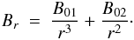 (3)The dual power-law form of Eq. (3) for
Br is the linear combination of a dipolar
field (∝ r-3), representing the dominant component of the global
solar magnetic field at solar minimum and a monopolar, solar wind component
(∝ r-2) prevailing at large distances from the Sun. Closer to
the Sun, higher-order multipole components are present, but their contribution can be
ignored at the heights relevant to these RM observations, since such fields fall off rapidly
with height. Analysis of Helios data (Mariani et al. 1979) showed that the absolute value of daily averages for the radial magnetic
field component scaled as
Br ∝ r-2
between 0.3 and 1 AU near solar minimum, which justifies the monopolar component in Eq. (3).
Moreover, the radial component of the heliospheric magnetic field, as detected by Ulysses
during the same solar minimum as the one investigated in this work, was found to be
remarkably constant with latitude, with an average value of
|Br| ≈ 3.1 × 10⁻⁵ G (Smith &
Balogh 1995; Balogh et al. 1995). In this paper, the value of B02,
representing the scale factor for the solar wind component
(∝ r-2) at great distances from the Sun, was therefore fixed
by this observational constraint, that is,
B02 ≈ 1.43 G × R⊙2
for Br, expressed in Gauss units
and r in solar radii (R⊙).
(3)The dual power-law form of Eq. (3) for
Br is the linear combination of a dipolar
field (∝ r-3), representing the dominant component of the global
solar magnetic field at solar minimum and a monopolar, solar wind component
(∝ r-2) prevailing at large distances from the Sun. Closer to
the Sun, higher-order multipole components are present, but their contribution can be
ignored at the heights relevant to these RM observations, since such fields fall off rapidly
with height. Analysis of Helios data (Mariani et al. 1979) showed that the absolute value of daily averages for the radial magnetic
field component scaled as
Br ∝ r-2
between 0.3 and 1 AU near solar minimum, which justifies the monopolar component in Eq. (3).
Moreover, the radial component of the heliospheric magnetic field, as detected by Ulysses
during the same solar minimum as the one investigated in this work, was found to be
remarkably constant with latitude, with an average value of
|Br| ≈ 3.1 × 10⁻⁵ G (Smith &
Balogh 1995; Balogh et al. 1995). In this paper, the value of B02,
representing the scale factor for the solar wind component
(∝ r-2) at great distances from the Sun, was therefore fixed
by this observational constraint, that is,
B02 ≈ 1.43 G × R⊙2
for Br, expressed in Gauss units
and r in solar radii (R⊙).
Helios observations also revealed that during solar minimum the slow solar wind of the streamer belt is restricted to a region of about ± 20° around the heliospheric current sheet. A similar result has been obtained by the Ulysses probe (e.g., Wock et al. 1997), which detected a sharp transition in latitude from slow to fast solar wind. Thus, in the following, we will assume for the sake of simplicity that the slow wind (streamer belt) region is confined in a region within 20° above and below the heliospheric neutral line, with the fast wind occurring beyond this latitudinally bounded region. Another important parameter is the Alfvén radius rA, that is, the distance at which the solar wind becomes super-Alfvénic in the outer corona. Below rA, the field is strong enough to control the plasma flow and cause the solar wind to corotate with the solar wind that has no azimuthal component in a corotating frame. Above rA, the plasma is released from corotation and the field wraps up approximately following an Archimedean spiral (Parker 1958). For r ≤ rA, in a spherical coordinate system (r,θ,φ) the azimuthal component of the magnetic field Bφ is null. Beyond rA, Bφ is different from zero, slowly growing with r as Bφ ∝ Ω⊙(r − rA)cosθ/usw, thus being a function of the coronal rotation rate Ω⊙, the solar wind speed usw, and of heliolatitude θ. The value of rA remains uncertain as yet, but it has been estimated to range from ~10 R⊙ over the poles to ~30 R⊙ over the equator (Scherer et al. 2001). In the following, rA is modeled by a step function assuming a value of rA = 30 R⊙ in the slow wind region around the equator and rA = 10 R⊙ in the fast wind region toward the poles.
Observations of the solar coronal rotation rate in solar cycle 23 have shown that the extended corona is more rigid than the photosphere (e.g., Giordano & Mancuso 2008; Mancuso & Giordano 2011, 2012), but is still sensibly latitude-dependent. We approximate the coronal rotation rate by the functional form given in Chandra et al. (2010) for the soft X-ray corona in 1997 from images obtained with the soft X-ray telescope (SXT) onboard the Yohkoh solar observatory. The value for the slow component of the solar wind speed was chosen on the basis of the average speed of the slow wind at 1 AU as deduced from the data obtained by the Solar Wind Experiment (SWE; Ogilvie et al. 1995) on the Wind spacecraft during May 1997. We relied on the analysis of Quemerais et al. (2007) for the fast solar wind at 1 AU, who deduced the velocity profiles for Spring 1997 from the combination of SWAN, LASCO, and IPS data. We remark that although for completeness we took into account the contribution of the azimuthal component of the magnetic field to the observed RM, this amount remains practically negligible (on the order of a few percent) in the range of heights considered in this work.
Finally, a necessary ingredient in coronal RM studies is the knowledge of the location of the heliospheric current sheet with respect to the LOS to the occulted radio sources. This information is important to infer the polarity of the magnetic field along the integration path to the different sources, especially near the solar equator. This is customarily achieved with PFSS models. Because of their simplicity, PFSS models are still used extensively within the solar and heliospheric communities. Riley et al. (2006) demonstrated that PFSS models are especially applicable during solar minimum activity and can generate solutions that closely match those generated by magnetohydrodynamic (MHD) models for cases when time-dependent phenomena are negligible. PFSS models assume that the magnetic field can be described as the negative gradient of the scalar potential Φ, which satisfies Laplace’s equation ∇2Φ = 0, thus implying that ∇ × B = 4πJ/c = 0, so that current densities J are neglected. Laplace’s equation for Φ is solved in the space between the photosphere and an outer spherical shell (the so-called source surface, with radius Rss), yielding a solution in terms of Legendre polynomials. The so-obtained scalar potential is uniquely determined given the inner and outer boundary conditions at the photosphere and at the source surface, respectively. The magnetic neutral line, when propagated outward, can be used as a proxy for the latitudinal location of the warped heliospheric current sheet, and this location can be readily and reliably obtained through the PFSS models. The coronal magnetic field calculated from photospheric field observations with the PFSS models is tabulated by the WSO and is available online at their website with two different extrapolation methods. The classic computation, which locates the source surface at 2.5 R⊙, assumes that the photospheric field has a meridional component and requires a somewhat ad hoc polar field correction to better match the in situ observations at 1 AU. The radial computation, with Rss located at 2.5 R⊙ and 3.25 R⊙, assumes that the field in the photosphere is radial and requires no polar field correction. The position of the magnetic neutral line, separating regions of opposite polarity, is simply given by the contour of zero magnetic field strength. In our model, the magnetic field is thus assumed to be almost purely radial above the source surface and a function only of radius except for the polarity-switching sign across the neutral line. The location of the heliospheric neutral sheet and, consequently, the polarity of the magnetic field, is inferred from the position of the magnetic neutral line as deduced from the three available PFSS models from WSO.
4. Results and discussion
In the following, we will implement three sets of models. In the first set of models (case A), we will use the functional form for the radial component of the heliospheric magnetic field given by Eq. (3) with B01 left as a free parameter to reproduce the observed RMs. We will furthermore assume that the radial variation of the electron density ne with heliographic coordinates can be reproduced with accuracy by the pB inversion method outlined in Sect. 2.2. This hypothesis might be questionable in that it would require both perfect calibration of the available LASCO C2 data and that the extrapolation to higher distances is accurate enough. In a second set of models (case B), we will set B01 = 0 and investigate the possibility that the electron density ne has been obtained only up to an unknown multiplicative factor Cn, so that its magnitude needs some adjustment (that is, ne → Cnne) to be in agreement with the actual RM observations (see also the discussion in Ingleby et al. 2007). By setting the parameter B01 to zero and letting Cn be the only free parameter, we will test the possibility that the radial magnetic field, down to a few solar radii from the Sun, might be simply described by a solar wind component (∝ r-2) (e.g., Vršnak et al. 2004; Spangler 2005; Ingleby et al. 2007). Finally, in the most general case (case C), both Cn and B01 will be left as free parameters. All these models will be separately tested by assuming the three available PFSS computations from WSO (i.e., the classic computation with Rss = 2.5 R⊙ and the radial computation with Rss = 2.5 R⊙ or 3.25 R⊙).
The unknown parameters in the above described models are evaluated by minimizing the
weighted sum-of-squared-residuals:  (4)where
RMobs,i is the observed RM
of the ith LOS,
RMi is the model RM for the
same LOS, and ωi is a weight assigned to each
measurement depending on its uncertainty. The proper choice of
ωi is a critical problem in our statistical
analysis. The available uncertainties σRM,i =
σi,obs (of about 0.1−0.3 rad m-2
for most observations)
for RMobs,i as quoted in
Mancuso & Spangler (2000) were assumed to be
solely due to radiometer noise. The RM fluctuations attributable to coronal turbulence and
MHD waves, δRM, can be much higher than
σRM,i, however. For example, RM
measurements from the Helios data showed RM fluctuations up to δRM
~ 2 rad m-2 with a time scale of roughly half an hour (Hollweg et al. 1982; Bird et al. 1985). Similarly, Sakurai & Spangler (1994) set an upper limit of δRM ~ 1.6 rad m-2
for a radio source observed during solar maximum whose LOS passed within
~9 R⊙ of the Sun, although Mancuso & Spangler (1999), in an analogous analysis near solar minimum, found
δRM ≲ 0.4 rad m-2. The overall level of
turbulent RM fluctuations is thus not well constrained as yet and might also depend on the
particular phase of the solar cycle. Since there was no simultaneous independent estimate of
the contribution of RM fluctuations attributable to coronal turbulence and MHD waves during
the days of observations, the uncertainties
σRM,i as quoted in Mancuso & Spangler
(2000) may underestimate the true
uncertainties in each measurement, given by
σRM,i
(4)where
RMobs,i is the observed RM
of the ith LOS,
RMi is the model RM for the
same LOS, and ωi is a weight assigned to each
measurement depending on its uncertainty. The proper choice of
ωi is a critical problem in our statistical
analysis. The available uncertainties σRM,i =
σi,obs (of about 0.1−0.3 rad m-2
for most observations)
for RMobs,i as quoted in
Mancuso & Spangler (2000) were assumed to be
solely due to radiometer noise. The RM fluctuations attributable to coronal turbulence and
MHD waves, δRM, can be much higher than
σRM,i, however. For example, RM
measurements from the Helios data showed RM fluctuations up to δRM
~ 2 rad m-2 with a time scale of roughly half an hour (Hollweg et al. 1982; Bird et al. 1985). Similarly, Sakurai & Spangler (1994) set an upper limit of δRM ~ 1.6 rad m-2
for a radio source observed during solar maximum whose LOS passed within
~9 R⊙ of the Sun, although Mancuso & Spangler (1999), in an analogous analysis near solar minimum, found
δRM ≲ 0.4 rad m-2. The overall level of
turbulent RM fluctuations is thus not well constrained as yet and might also depend on the
particular phase of the solar cycle. Since there was no simultaneous independent estimate of
the contribution of RM fluctuations attributable to coronal turbulence and MHD waves during
the days of observations, the uncertainties
σRM,i as quoted in Mancuso & Spangler
(2000) may underestimate the true
uncertainties in each measurement, given by
σRM,i , by some factor. As a consequence, the true
uncertainties σRM,i∗ remain unknown.
According to the previous discussion, in the process of χ2
minimization for the evaluation of the unknown parameters, we considered different
ωi estimates by proceeding through three
different steps, as explained below.
, by some factor. As a consequence, the true
uncertainties σRM,i∗ remain unknown.
According to the previous discussion, in the process of χ2
minimization for the evaluation of the unknown parameters, we considered different
ωi estimates by proceeding through three
different steps, as explained below.
First of all, in step 1 we analyzed the RM data by considering as their total uncertainties
σRM,i the ones that can be ascribed to
radiometric noise only, i.e., we completely neglected the possible contribution of coronal
turbulence and MHD waves to RM fluctuations. We minimized the χ2
for each of the cases A, B, and C and for each available PFSS model. We then computed the
reduced chi-squared  by taking into account the number of degrees
of freedom (ν) in the different cases (12 for cases A and B, and 11 for
case C, due to the different number of estimated parameters). We also estimated the
goodness-of-fit by computing the probability of observing a minimum of the distribution that
arises from Eq. (4) by varying the model parameters, larger than the one observed, assuming
that this minimum is distributed according to a χ2 with
ν degrees of freedom (e.g., Garzelli & Giunti 2002). Calling α this probability, which in practice
represents the area of the right tail of the χ2 distribution in
the interval between [
by taking into account the number of degrees
of freedom (ν) in the different cases (12 for cases A and B, and 11 for
case C, due to the different number of estimated parameters). We also estimated the
goodness-of-fit by computing the probability of observing a minimum of the distribution that
arises from Eq. (4) by varying the model parameters, larger than the one observed, assuming
that this minimum is distributed according to a χ2 with
ν degrees of freedom (e.g., Garzelli & Giunti 2002). Calling α this probability, which in practice
represents the area of the right tail of the χ2 distribution in
the interval between [ and + ∞), we assumed this fit to be
acceptable at 100% α confidence level. In all cases, the reduced
chi-squared for the best-fit points were
and + ∞), we assumed this fit to be
acceptable at 100% α confidence level. In all cases, the reduced
chi-squared for the best-fit points were  , thus yielding a very poor
α. These results clearly suggest that the uncertainty component due to
radiometric noise largely underestimates the total uncertainty, at least for some of the
sources, and that the uncertainties δRM due to RM fluctuations cannot be
neglected in our study. Secondly, in step 2, in the absence of an experimental estimate of
δRM for the measurements at hand, we considered the range of possible
δRM estimates provided in the literature (see the discussion above) to
obtain a gross estimate of the typical order of magnitude of δRM. Taking
into account the interval spanned by these estimates, we decided to adopt an average value
δRM = 1 rad m-2 that we assumed to remain constant during the
days of our RM observations. We also assumed that, as expected in a realistic situation, the
RM fluctuations do not act by systematically increasing or by systematically decreasing all
RM observed values in the same direction, but may act in a different way on each RM
observation, i.e., they do not introduce any correlation between the RM observations of
different sources. We thus replaced the uncertainties
σRM,i =
σi,obs used in step 1 with the
uncertainties
σRM,i
, thus yielding a very poor
α. These results clearly suggest that the uncertainty component due to
radiometric noise largely underestimates the total uncertainty, at least for some of the
sources, and that the uncertainties δRM due to RM fluctuations cannot be
neglected in our study. Secondly, in step 2, in the absence of an experimental estimate of
δRM for the measurements at hand, we considered the range of possible
δRM estimates provided in the literature (see the discussion above) to
obtain a gross estimate of the typical order of magnitude of δRM. Taking
into account the interval spanned by these estimates, we decided to adopt an average value
δRM = 1 rad m-2 that we assumed to remain constant during the
days of our RM observations. We also assumed that, as expected in a realistic situation, the
RM fluctuations do not act by systematically increasing or by systematically decreasing all
RM observed values in the same direction, but may act in a different way on each RM
observation, i.e., they do not introduce any correlation between the RM observations of
different sources. We thus replaced the uncertainties
σRM,i =
σi,obs used in step 1 with the
uncertainties
σRM,i , finding
 values compatible with 1, thus leading to a
more meaningful statistical analysis. In this configuration, we were able to identify the
best PFSS model among those proposed by the WSO (that turned out to be the same for all
three cases A, B and C), the best-fit parameters for each case, and the uncertainties on
them at the 90%, 95%, and 99% confidence levels. These uncertainties are given in the
following as confidence intervals in the cases where we just varied a single parameter
(cases A and B), and as confidence regions when, instead, we varied more parameters at the
same time (case C). Finallly, in step 3, we considered a statistical analysis with uniform
weighting, i.e., with ωi arbitrarily set to 1,
so that it yields an unweighted least-squares. The results of this analysis turned out to be
similar to those of the analysis of step 2, which proves the marginal role of
σi,obs on the analysis’ outcome with respect
to the dominant contribution from turbulence and MHD waves (i.e,
σRM,i ∗ ≈ δRM ≫ σi,obs).
values compatible with 1, thus leading to a
more meaningful statistical analysis. In this configuration, we were able to identify the
best PFSS model among those proposed by the WSO (that turned out to be the same for all
three cases A, B and C), the best-fit parameters for each case, and the uncertainties on
them at the 90%, 95%, and 99% confidence levels. These uncertainties are given in the
following as confidence intervals in the cases where we just varied a single parameter
(cases A and B), and as confidence regions when, instead, we varied more parameters at the
same time (case C). Finallly, in step 3, we considered a statistical analysis with uniform
weighting, i.e., with ωi arbitrarily set to 1,
so that it yields an unweighted least-squares. The results of this analysis turned out to be
similar to those of the analysis of step 2, which proves the marginal role of
σi,obs on the analysis’ outcome with respect
to the dominant contribution from turbulence and MHD waves (i.e,
σRM,i ∗ ≈ δRM ≫ σi,obs).
The results obtained using the weighting criteria of steps 2 and 3 are from a physical point of view more representative of the real situation, insofar the true uncertainties are most probably dominated by the contribution of RM fluctuations attributable to coronal turbulence and MHD waves. In the following, we therefore concentrate our discussion mostly on the results from steps 2 and 3. We remark, however, that the above conclusion is strictly valid only assuming (which is yet to be verified in the range of heliocentric distances considered in this work) that δRM ~ constant both in latitude and distance from the Sun.
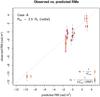 |
Fig. 2 Scatter plot of predicted RMs versus observed RMs in the best-fit parameter configuration, using a model with B01 left as free parameter and setting Cn = 1. Results are displayed for the two cases of non-uniform weights, after the two analyses described in step 1 (yellow squares) and step 2 (green circles), respectively. The dashed 1:1 line shows the diagonal, corresponding to the ideal situation where predicted and measured values are equal. The solid (red and brown) error bars denote the σRM,i uncertainties for each measurement due to radiometer noise as quoted in Mancuso & Spangler (2000), whereas the dashed (blue) errorbars denote the σRM,i∗ total uncertainties obtained after adding the contribution of RM fluctuations, estimated to be δRM = 1 rad m-2 for the sake of this analysis. |
4.1. Model with B01 ≠ 0 and Cn = 1 (case A)
To find the regions of parameter space that are consistent with the RM observations, we performed a first grid search allowing the two unknown parameters B01 and Rss to vary within a plausible range and fixing the multiplicative factor Cn to unity (that is, assuming that the radial variation of the electron density with heliographic coordinates is reproduced with accuracy). The ranges of the model parameters that define our search space were constrained to be within a plausible interval of 0 < B01 < 20 (with B01 expressed hereafter in units of G × R⊙3) at steps of 0.01 R⊙. The result of the best-fitting procedure yielded a very well defined χ2 minimum, thus allowing an accurate determination of the best-fit parameters. The best-fit parameters to the observed data for case A are B01 = 10.54 and B01 = 10.95 for the two weighing criteria explained above (steps 2 and 3) and for the radial computation with Rss = 2.5 R⊙. The radial computation with Rss = 3.25 R⊙ yields higher χ2 values, while the classic computation with Rss = 2.5 R⊙ yields a very high χ2 value, hinting at B01 = 0. How well a model performs compared with the measurements is conveniently assessed from the scatter plot of observations versus predictions. Tighter scatter of the data points around the 1:1 line obviously indicates a more accurate model fit. In Fig. 2, we show a scatter plot of predicted RMs versus observed RMs for case A obtained by using the best-fitting parameters and the two non-uniform weighting criteria listed in steps 1 and 2. The estimated RM values look to be nicely distributed around the line 1:1 of the perfect fit for the whole range of measured RM values. The largest discrepancies between the results of the models of steps 1 and 2, which differ because of the RM uncertainties attributed to each observation, also shown in the plot, are visible in the RM predictions for the sources that have a higher absolute experimental RM value. In particular, adopting the model of step 2 appears to greatly improve the agreement between theory and experiment for the source with an highly negative measured RM (<–10 rad m-2).
Best-fit models. See text for more detail.
4.2. Model with B01 = 0 and Cn ≠ 1 (case B)
In the model presented in the previous section (case A), we assumed that the radial variation of the electron density with heliographic coordinates could be reproduced with accuracy by the pB inversion method applied to the white-light data, thus requiring perfect calibration of the available data and accuracy in the extrapolation of the LASCO C2 data to higher distances. As already mentioned, however, the electron density ne can probably be retrieved, at best, only up to an unknown multiplicative factor Cn, representing an adjustment factor introduced to produce agreement with the actual RM observations (see also the discussion in Ingleby et al. 2007). Accordingly, in the second model (case B), we performed a grid search by setting B01 = 0 (that is, assuming no dipolar component), allowing the parameter Cn to vary within a plausible interval of 0.3 <Cn < 3 at steps of 0.01 R⊙. This model was implemented to test the possibility that the radial component of the magnetic field might be already ∝ r-2 at distances as low as a few solar radii from the Sun (e.g., Vršnak et al. 2004; Spangler 2005; Ingleby et al. 2007). The best-fit parameter to the observed data for case B is Cn = 2.00 for the radial computation with Rss = 2.5 R⊙. Again, the radial computation with Rss = 3.25 R⊙ yields higher χ2 values, while the classic computation with Rss = 2.5 R⊙ yields a very high χ2 value, hinting to low Cn values. The scatter plot of predicted versus observed RMs, with predictions obtained by using the best-fitting parameters for this case, assuming a PFSS radial computation with Rss = 2.5 R⊙ is shown in Fig. 3. Considerations similar to those concerning Fig. 2 are valid (see the discussion at the end of the previous subsection).
4.3. Model with B01 ≠ 0 and Cn ≠ 1 (case C)
In the last model (case C), we additionally performed a grid search allowing the two
unknown parameters B01 and
Cn to vary within the intervals
0 < B01 < 40 and
0.3 < Cn < 3. In this case, a
minimum χ2 was also very well defined, allowing us to
accurately determine the best-fit parameters. The model parameters that provide the best
fit to the observed data are B01 = 4.84 and
Cn = 1.39 for
 , and
B01 = 6.46 and
Cn = 1.28 for
ωi = 1. Again, the best-fit was obtained
for the radial computation with
Rss = 2.5 R⊙. In Fig. 4, we show
the scatter plot of predicted versus observed RMs obtained by using the best-fitting
parameters. Considerations similar to those concerning Fig. 2 apply even in this case.
, and
B01 = 6.46 and
Cn = 1.28 for
ωi = 1. Again, the best-fit was obtained
for the radial computation with
Rss = 2.5 R⊙. In Fig. 4, we show
the scatter plot of predicted versus observed RMs obtained by using the best-fitting
parameters. Considerations similar to those concerning Fig. 2 apply even in this case.
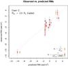 |
Fig. 4 Same as Fig. 3, but using a model with both B01 and Cn left as free parameters. |
4.4. Discussion and comparison with other models
The model results are summarized in Table 1. For comparative purposes, for each
considered model, the parameters Cn and
B01 that provided the best-fit to the observed RMs are
tabulated together with the corresponding best-fit for the cases of non-uniform
(ωi and
ωi
and
ωi ) and uniform
(ωi ≡ 1) weighting, corresponding to the
three steps outlined above for the evaluation of the uncertainties. We also report the
estimate of α for the models for which it is higher than 1%. We remark
that the values of this variable strictly depend on the above hypotheses concerning the RM
uncertainties (see the discussion before Sect. 4.1), thus it has to be considered with
some care. For the model in the last line of Table 1 (classic computation with
Rss = 2.5), we found that the χ2
is minimized by choosing very high values of the B01
component, beyond the physical limits expected to be plausible on the basis of current
knowledge, so this model has probably to be ruled out.
) and uniform
(ωi ≡ 1) weighting, corresponding to the
three steps outlined above for the evaluation of the uncertainties. We also report the
estimate of α for the models for which it is higher than 1%. We remark
that the values of this variable strictly depend on the above hypotheses concerning the RM
uncertainties (see the discussion before Sect. 4.1), thus it has to be considered with
some care. For the model in the last line of Table 1 (classic computation with
Rss = 2.5), we found that the χ2
is minimized by choosing very high values of the B01
component, beyond the physical limits expected to be plausible on the basis of current
knowledge, so this model has probably to be ruled out.
Overall, among the nine considered models (see Table 1), the three of them obtained by
assuming the position of the magnetic neutral line as deduced from the radial
computation with
Rss = 2.5 R⊙ always yielded the
lowest minimum for all weighting criteria. For the two
weighting criteria of steps 2 and 3, we obtained values of
at the minima that were low enough to
allow for a meaningful statistical analysis (α > 1−2%). The models
computed by assuming the radial computation with
Rss = 3.25 R⊙ also yielded
well-defined χ2 minima within the allowed parameter space,
although with higher χ2 minimum values and with lower
α values with respect to the radial computation with
Rss = 2.5 R⊙. Finally, the
classic computation always yielded the highest
minimum χ2 (often at the border of the parameter space) and
the poorest α among the three available WSO models. These results allow
us to clearly draw our first and more robust conclusion, that is, that the radial
computation of the PFSS model from WSO with a source surface located at
2.5 R⊙ is indeed the preferred choice, at least near solar
minimum.
Reconsidering Table 1, it turns out that the minimum χ2 for
case C is always lower than that for case A and B for all weighting criteria. We remark,
however, that this inequality is no longer true when comparing case C and case A by
considering the instead of the
χ2, because of the different ν, although in
both cases ~ 1 for the radial
computation with
Rss = 2.5 R⊙. Related to this,
the α value for case A turns out, indeed, to be slightly higher than that
of case C. However, the difference is quite small for the two weighting criteria of
steps 2 and 3, and thus we believe that both fits deserve full consideration. On the other
hand, the α value of case B appears to be slightly poorer, especially in
the case of the weighting criterium of step 3. Following the indications of our
statistical analysis, we consider, for the sake of comparison of our results with other
magnetic field estimates in the literature, both the models of case A and C. On the other
hand, taking into account the intrinsic uncertanties and assumptions related to the
pB-inversion method used in this work, we are aware that our density
estimate certainly needs some adjustment, at best by means of an
enhancement or depletion factor. Probably the slightly higher α value for
case A with respect to case C is just an artifact related to the fact that
our χ2 distributions are shallow. This impression is
confirmed by comparing our results in the two cases with independent work published in the
literature, as explained in the following.
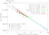 |
Fig. 5 Comparison of the result from this work, Eqs. (5) and (6), with various estimates (plotted with different symbols and colors) for the radial profile of the magnetic field strength in the inner heliosphere. |
Our best-fit model for case A, expressed as a power-law fit valid in the range between
about 5 and 14 R⊙, is
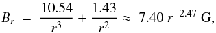 (5)whereas our best-fit model for case C,
expressed as a power-law fit valid in the range between about 5
and 14 R⊙, is
(5)whereas our best-fit model for case C,
expressed as a power-law fit valid in the range between about 5
and 14 R⊙, is
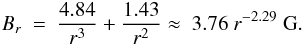 (6)Several empirical formulas have been
introduced in literature in the past decades to model the radial magnetic field profile.
In Fig. 5, we compare the magnetic field radial profile as derived from this work, given
by Eqs. (5) and (6), with the radial profiles obtained in the inner heliosphere by Dulk
& McLean (1978), Pätzold et al. (1987), Vršnak et al. (2004), Gopaswamy & Yashiro (2011), and Poomvises et al. (2012) with different techniques. Specifically, Dulk
& McLean (1978) derived, from radio
observations, a radial profile given by
Br = 0.5 (r − 1)-1.5 G
for r < 10 R⊙. The estimate by Pätzold
et al. (1987),
Br = 7.9 r-2.7 G,
valid in the range between 3 and 10 R⊙, was also obtained
through Faraday rotation measurements but using data from Helios. Vršnak et al. (2004) used information on the band splitting of type II
radio bursts, obtaining
Br = 1.4 r-1.97 G
from the corona up to 1 AU. In the same plot, we also show additional estimates of the
magnetic field strength in the inner heliosphere with various symbols (Sakurai &
Spangler 1994; Spangler 2005; Ingleby et al. 2007; Feng
et al. 2011; You et al. 2012). From Fig. 5, it can be appreciated that the magnitude and
variation trend of the radial component of the magnetic field as obtained in our analysis,
case C, agrees fairly well with the other estimates and in particular with the result from
Pätzold et al. (1987), at least in the range of
heights around 5 R⊙, which is somewhat steeper overall.
Moreover, the match with the estimate of Poomvises et al. (2012), obtained with a completely different method, i.e., from the analysis of
the standoff distance of a CME-driven shock observed by the Solar Terrestrial Relations
Observatory (STEREO) spacecraft, is particularly interesting. On the other hand, the
magnetic field profile we obtained instead by assuming
Cn = 1 (case A) appears to overestimate
all other results, although its extrapolation at higher heights still agrees fairly well
with the estimate of Poomvises et al. (2012). This
substantiates our hypothesis that the ne as estimated by means
of the pB-inversion method needs some correction (as suggested by the
introduction of the enhancement factor Cn),
and that our best estimate of the radial magnetic field profile in the inner heliosphere
is given by Eq. (6) and not Eq. (5). Finally, we remark that the radial profile obtained
by Gopalswamy & Yashiro (2011), who analyzed
the shock stand-off distance and the radius of curvature of a flux rope associated to a
CME event, is instead much flatter than our profile. When comparing the above radial
magnetic field estimates, however, we recall that all of them were obtained through
remote-sensing techniques and are therefore strongly influenced by the assumed (or, at
best, estimated) electron density distribution along the LOS.
(6)Several empirical formulas have been
introduced in literature in the past decades to model the radial magnetic field profile.
In Fig. 5, we compare the magnetic field radial profile as derived from this work, given
by Eqs. (5) and (6), with the radial profiles obtained in the inner heliosphere by Dulk
& McLean (1978), Pätzold et al. (1987), Vršnak et al. (2004), Gopaswamy & Yashiro (2011), and Poomvises et al. (2012) with different techniques. Specifically, Dulk
& McLean (1978) derived, from radio
observations, a radial profile given by
Br = 0.5 (r − 1)-1.5 G
for r < 10 R⊙. The estimate by Pätzold
et al. (1987),
Br = 7.9 r-2.7 G,
valid in the range between 3 and 10 R⊙, was also obtained
through Faraday rotation measurements but using data from Helios. Vršnak et al. (2004) used information on the band splitting of type II
radio bursts, obtaining
Br = 1.4 r-1.97 G
from the corona up to 1 AU. In the same plot, we also show additional estimates of the
magnetic field strength in the inner heliosphere with various symbols (Sakurai &
Spangler 1994; Spangler 2005; Ingleby et al. 2007; Feng
et al. 2011; You et al. 2012). From Fig. 5, it can be appreciated that the magnitude and
variation trend of the radial component of the magnetic field as obtained in our analysis,
case C, agrees fairly well with the other estimates and in particular with the result from
Pätzold et al. (1987), at least in the range of
heights around 5 R⊙, which is somewhat steeper overall.
Moreover, the match with the estimate of Poomvises et al. (2012), obtained with a completely different method, i.e., from the analysis of
the standoff distance of a CME-driven shock observed by the Solar Terrestrial Relations
Observatory (STEREO) spacecraft, is particularly interesting. On the other hand, the
magnetic field profile we obtained instead by assuming
Cn = 1 (case A) appears to overestimate
all other results, although its extrapolation at higher heights still agrees fairly well
with the estimate of Poomvises et al. (2012). This
substantiates our hypothesis that the ne as estimated by means
of the pB-inversion method needs some correction (as suggested by the
introduction of the enhancement factor Cn),
and that our best estimate of the radial magnetic field profile in the inner heliosphere
is given by Eq. (6) and not Eq. (5). Finally, we remark that the radial profile obtained
by Gopalswamy & Yashiro (2011), who analyzed
the shock stand-off distance and the radius of curvature of a flux rope associated to a
CME event, is instead much flatter than our profile. When comparing the above radial
magnetic field estimates, however, we recall that all of them were obtained through
remote-sensing techniques and are therefore strongly influenced by the assumed (or, at
best, estimated) electron density distribution along the LOS.
5. Summary and conclusions
Faraday rotation measures estimated by Mancuso & Spangler (2000) along thirteen LOS to ten extragalactic radio sources occulted by the corona were used to constrain the inner heliospheric magnetic field around solar minimum. Since RM observations basically probe the electron density-weighted magnetic field strength along the integration path, the crucial point in this type of analysis is to obtain a reliable estimate of the intervening electron density distribution along each LOS.
By inverting LASCO/SOHO pB data, we were able to separate the two plasma properties that contribute to the observed RMs, thus allowing the radial component of the inner heliospheric magnetic field, assumed to have a simple analytical form, to be uniquely determined. By comparing observed and model RM values, using a best-fitting procedure, we found that this profile can be nicely approximated by a power-law of the form Br = 3.76 r-2.29 G, in a range of heights spanning from about 5 to 14 R⊙. To obtain this estimate, an enhancement factor of Cn ≈ 1.3 was required for the electron density ne as inferred by means of the pB-inversion technique. The magnitude and variation trend of the radial component of the magnetic field as obtained in our analysis agrees fairly well with previous estimates. Finally, our analysis suggests that the radial computation of the PFSS model from the WSO with a source surface located at Rss = 2.5 R⊙ is the preferred choice near solar minimum.
Future direct measurements of the magnetic field from the magnetometers onboard NASA’s Solar Probe Plus mission are expected to additionally constrain the magnetic field radial profile in the range of heights investigated in this work.
Solar Probe Plus website, http://solarprobe.jhuapl.edu/
Acknowledgments
The authors would like to thank the anonymous referee for the very helpful comments and suggestions that significantly improved the paper. M.V. Garzelli is grateful to C. Giunti for many useful discussions and suggestions concerning the statistical analysis of the data shown in this paper. Special thanks to S.R. Spangler for the inspiration of this work. The SOHO/LASCO pB data used in this work are produced by a consortium of the Naval Research Laboratory (USA), the Max-Planck-Institut für Aeronomie (Germany), the Laboratoire d’Astronomie Spatiale (France), and the University of Birmingham (UK). SOHO is a project of international cooperation between ESA and NASA. The NRAO is a facility of the NSF operated under cooperative agreement by Associated Universities, Inc. Wilcox Solar Observatory data used in this work were obtained via the WSO website, courtesy of J. T. Hoeksema. The WSO is supported by NASA, the National Science Foundation, and ONR.
References
- Altschuler, M. D., & Newkirk, G. 1969, Sol. Phys., 9, 131 [Google Scholar]
- Balogh, A., Smith, E. J., Tsurutani, B. T., et al. 1995, Science, 268, 1007 [NASA ADS] [CrossRef] [Google Scholar]
- Bemporad, A., & Mancuso, S. 2010, ApJ, 720, 130 [NASA ADS] [CrossRef] [Google Scholar]
- Bird, M. K. 2007, Astron. Astroph. Trans., 26, 441 [NASA ADS] [CrossRef] [Google Scholar]
- Bird, M. K., Volland, H., Howard, R. A., et al. 1985, Sol. Phys., 98, 341 [NASA ADS] [CrossRef] [Google Scholar]
- Brueckner, G. E., Howard, R. A., Koomen, M. J., et al. 1995, Sol. Phys., 162, 357 [NASA ADS] [CrossRef] [Google Scholar]
- Chandra, S., Vats, H. O., & Iyer, K. N. 2010, MNRAS, 407, 1108 [NASA ADS] [CrossRef] [Google Scholar]
- Chiu, Y. T. 1975, J. Atmos. Terr. Phys, 37, 1563 [Google Scholar]
- Cho, K.-S., Lee, J., Gary, D. E., Moon, Y.-J., & Park, Y. D. 2007, ApJ, 665, 799 [NASA ADS] [CrossRef] [Google Scholar]
- Domingo, V., Fleck, B., & Poland, A. I. 1995, Sol. Phys., 162, 1 [NASA ADS] [CrossRef] [Google Scholar]
- Dulk, G. A., & McLean, D. J. 1978, Sol. Phys., 57, 279 [NASA ADS] [CrossRef] [Google Scholar]
- Feng, S. W., Chen, Y., Li, B., et al. 2011, Sol. Phys., 272, 119 [NASA ADS] [CrossRef] [Google Scholar]
- Gary, G. A. 2001, Sol. Phys., 203, 71 [NASA ADS] [CrossRef] [Google Scholar]
- Garzelli, M. V., & Giunti C., 2002, Astropart. Phys. 17, 205 [NASA ADS] [CrossRef] [Google Scholar]
- Gibson, S. E., Fludra, A., Bagenal, F., et al. 1999, J. Geophys. Res., 104, 9691 [NASA ADS] [CrossRef] [Google Scholar]
- Giordano, S., & Mancuso, S. 2008, ApJ, 688, 656 [NASA ADS] [CrossRef] [Google Scholar]
- Gopalswamy, N., & Yashiro, S. 2011, ApJ, 736, L17 [Google Scholar]
- Guhathakurta, M., Holzer, T. E., & MacQueen, R. M. 1996, ApJ, 458, 817 [NASA ADS] [CrossRef] [Google Scholar]
- Hoeksema, J. T., Wilcox, J. M., & Scherrer, P. H. 1983, J. Geophys. Res., 88, 9910 [NASA ADS] [CrossRef] [Google Scholar]
- Hollweg, J. V., Bird, M. K., Volland, H., et al. 1982, J. Geophys. Res., 87, 1 [NASA ADS] [CrossRef] [Google Scholar]
- Ingleby, L. D., Spangler, S. R., & Whiting, C. A. 2007, ApJ, 668, 520 [NASA ADS] [CrossRef] [Google Scholar]
- Kim, R.-S., Gopalswamy, N., Moon, Y.-J., Cho, K.-S., & Yashiro, S. 2012, ApJ, 746, 118 [NASA ADS] [CrossRef] [Google Scholar]
- Koutchmy, S., & Lamy, P. L. 1985, in Properties and Interactions of Interplanetary Dust, eds. R. H. Giese, & P. Lamy (Dordrecht: Reidel), IAU Colloq., 85, 63 [Google Scholar]
- Jensen, E. A., Bird, M. K., Asmar, S. W., et al. 2005, Adv. Space Res., 36, 1587 [NASA ADS] [CrossRef] [Google Scholar]
- Lee, J. 2007, Space Sci. Rev., 133, 73 [NASA ADS] [CrossRef] [Google Scholar]
- Lin, H., Penn, M. J., & Tomczyk, S. 2000, ApJ, 541, L83 [NASA ADS] [CrossRef] [Google Scholar]
- Mancuso, S., & Garzelli, M. V. 2007, A&A, 466, L5 [NASA ADS] [CrossRef] [EDP Sciences] [Google Scholar]
- Mancuso, S., & Giordano, S. 2011, ApJ, 729, 79 [NASA ADS] [CrossRef] [Google Scholar]
- Mancuso, S., & Giordano, S. 2012, A&A, 539, A26 [NASA ADS] [CrossRef] [EDP Sciences] [Google Scholar]
- Mancuso, S., & Spangler, S. R. 1999, ApJ, 525, 195 [NASA ADS] [CrossRef] [Google Scholar]
- Mancuso, S., & Spangler, S. R. 2000, ApJ, 539, 480 [NASA ADS] [CrossRef] [Google Scholar]
- Mancuso, S., Raymond, J. C., Kohl, J., et al. 2003, A&A, 400, 347 [NASA ADS] [CrossRef] [EDP Sciences] [Google Scholar]
- Mann, I. 1992, A&A, 261, 329 [NASA ADS] [Google Scholar]
- Mariani, F., Villante, U., Bruno, R., Bavassano, B., & Ness, N. F. 1979, Sol. Phys., 63, 411 [NASA ADS] [CrossRef] [Google Scholar]
- Morrill, J. S., Korendyke, C. M., Brueckner, G. E., et al. 2006, Sol. Phys., 233, 331 [Google Scholar]
- Ogilvie, K. W., Chornay, D. J., Fritzenreiter, R. J., et al. 1995, Space Sci. Rev., 71, 55 [NASA ADS] [CrossRef] [Google Scholar]
- Ord, S. M., Johnston, S., & Sarkissian, J. 2007, Sol. Phys., 245, 109 [NASA ADS] [CrossRef] [Google Scholar]
- Parker, E. N. 1958, ApJ, 128, 664 [Google Scholar]
- Pätzold, M., Bird, M. K., Volland, H., et al. 1987, Sol. Phys., 109, 91 [NASA ADS] [CrossRef] [Google Scholar]
- Poomvises, W., Gopalswamy, N., Yashiro, S., Kwon, R.-Y., & Olmedo, O. 2012, ApJ, 758, 118 [NASA ADS] [CrossRef] [Google Scholar]
- Quemerais, E., Lallement, R., Koutroumpa, D., & Lamy, P. 2007, ApJ, 667, 1229 [NASA ADS] [CrossRef] [Google Scholar]
- Riley, P., Linker, J. A., Mikic, Z., et al. 2006, ApJ, 653, 1510 [Google Scholar]
- Sakurai, T., & Spangler, S. R., 1994, ApJ, 434, 773 [NASA ADS] [CrossRef] [Google Scholar]
- Schatten, K. H., Wilcox, J. M., & Ness, N. F. 1969, Sol. Phys., 6, 442 [Google Scholar]
- Scherer, K., Marsch, E., Schwenn, R., & Rosenbauer, H. 2001, A&A, 366, 331 [NASA ADS] [CrossRef] [EDP Sciences] [Google Scholar]
- Smith, E. J., & Balogh, A. 1995, Geophys. Res. Lett., 22, 3317 [NASA ADS] [CrossRef] [Google Scholar]
- Spangler, S. R. 2005, Space Sci. Rev., 121, 189 [NASA ADS] [CrossRef] [Google Scholar]
- Stelzried, C. T., Levy, G. S., Sato, T., et al. 1970, Sol. Phys., 14, 440 [NASA ADS] [CrossRef] [Google Scholar]
- van de Hulst, H. C. 1950, Bull. Astron. Inst. Netherlands, 11, 135 [Google Scholar]
- Vršnak, B., Magdalenic, J., & Zlobec, P. 2004, A&A, 413, 753 [NASA ADS] [CrossRef] [EDP Sciences] [Google Scholar]
- Woch, J., Axford, W. I., Mall, U., et al. 1997, Geophys. Res. Lett., 24, 2885 [NASA ADS] [CrossRef] [Google Scholar]
- You, X. P., Coles, W. A., Hobbs, G. B., & Manchester, R. N. 2012, MNRAS, 422, 1160 [NASA ADS] [CrossRef] [Google Scholar]
All Tables
All Figures
|
Fig. 1 Location of the radio sources relative to the Sun on each of the four days of observation. The bull’s eye symbol indicates the position of the Sun and the dotted line is the ecliptic. The size of the plotted symbol is a rough indicator of the absolute magnitude of the RM. Red squares correspond to positive RMs and blue circles represent negative RMs. |
| In the text | |
|
Fig. 2 Scatter plot of predicted RMs versus observed RMs in the best-fit parameter configuration, using a model with B01 left as free parameter and setting Cn = 1. Results are displayed for the two cases of non-uniform weights, after the two analyses described in step 1 (yellow squares) and step 2 (green circles), respectively. The dashed 1:1 line shows the diagonal, corresponding to the ideal situation where predicted and measured values are equal. The solid (red and brown) error bars denote the σRM,i uncertainties for each measurement due to radiometer noise as quoted in Mancuso & Spangler (2000), whereas the dashed (blue) errorbars denote the σRM,i∗ total uncertainties obtained after adding the contribution of RM fluctuations, estimated to be δRM = 1 rad m-2 for the sake of this analysis. |
| In the text | |
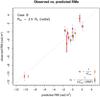 |
Fig. 3 Same as Fig. 2, but using a model with Cn left as free parameters and setting B01 = 0. |
| In the text | |
|
Fig. 4 Same as Fig. 3, but using a model with both B01 and Cn left as free parameters. |
| In the text | |
|
Fig. 5 Comparison of the result from this work, Eqs. (5) and (6), with various estimates (plotted with different symbols and colors) for the radial profile of the magnetic field strength in the inner heliosphere. |
| In the text | |
Current usage metrics show cumulative count of Article Views (full-text article views including HTML views, PDF and ePub downloads, according to the available data) and Abstracts Views on Vision4Press platform.
Data correspond to usage on the plateform after 2015. The current usage metrics is available 48-96 hours after online publication and is updated daily on week days.
Initial download of the metrics may take a while.