| Issue |
A&A
Volume 553, May 2013
|
|
|---|---|---|
| Article Number | A8 | |
| Number of page(s) | 15 | |
| Section | Planets and planetary systems | |
| DOI | https://doi.org/10.1051/0004-6361/201219013 | |
| Published online | 18 April 2013 | |
The HARPS search for southern extra-solar planets
XXXIII. Super-Earths around the M-dwarf neighbors Gl 433 and Gl 667C⋆,⋆⋆
1 UJF-Grenoble 1/CNRS-INSU, Institut de Planétologie et d’Astrophysique de Grenoble (IPAG) UMR 5274, 38041 Grenoble, France
e-mail: This email address is being protected from spambots. You need JavaScript enabled to view it.
2 Observatoire de Genève, Université de Genève, 51 ch. des Maillettes, 1290 Sauverny, Switzerland
3 Institut d’Astrophysique de Paris, CNRS, Université Pierre et Marie Curie, 98bis Bd. Arago, 75014 Paris, France
4 Université de Liège, Allée du 6 août 17, Sart Tilman, Liège 1, Belgium
5 Centro de Astrofísica, Universidade do Porto, Rua das Estrelas, 4150-762 Porto, Portugal
6 Departamento de Física e Astronomia, Faculdade de Ciências, Universidade do Porto, Rua do Campo Alegre, 4169-007 Porto, Portugal
Received: 10 February 2012
Accepted: 30 July 2012
Abstract
Context. M dwarfs have often been found to have super-Earth planets with short orbital periods. These stars are thus preferential targets in searches for rocky or ocean planets in the solar neighborhood.
Aims. Our research group recently announced the discovery of one and two low-mass planets around the M1.5V stars Gl 433 and Gl 667C, respectively. We found these planets with the HARPS spectrograph on the ESO 3.6-m telescope at La Silla Observatory, from observations obtained during the guaranteed time observing program of that instrument.
Methods. We obtained additional HARPS observations of those two stars, for a total of 67 and 179 radial velocity measurements for Gl 433 and Gl 667C, respectively, and present here an orbital analysis of these extended data sets and our main conclusions about both planetary systems.
Results. One of the three planets, Gl 667Cc, has a mass of only M2sini ~ 4.25 M⊕ and orbits in the central habitable zone of its host star. It receives only 10% less stellar energy from Gl 667C than the Earth receives from the Sun. However, planet evolution in the habitable zone can be very different if the host star is a M dwarf or a solar-like star, without necessarily questioning the presence of water. The two other planets, Gl 433b and Gl 667Cb, both have M2sini of ~5.5 M⊕ and periods of ~7 days. The radial velocity measurements of both stars contain longer timescale signals, which we fit with longer period Keplerians. For Gl 433, the signal probably originates in a magnetic cycle, while data of longer time span will be needed before conclusive results can be obtained for Gl 667C. The metallicity of Gl 433 is close to solar, while Gl 667C is metal poor with [Fe/H] ~ −0.6. This reinforces the recent conclusion that the occurrence of super-Earth planets does not strongly correlate with the stellar metallicity.
Key words: techniques: radial velocities / planets and satellites: detection / stars: late-type
Based on observations collected with HARPS instrument on the 3.6-m telescope at La Silla Observatory (European Southern Observatory) under programs ID072.C-0488(E).
Appendix A is available in electronic form at http://www.aanda.org
© ESO, 2013
1. Introduction
Much interest has recently focused on planets around M dwarfs, with three main motivations: constraining formation, constraining the physico-chemistry of planets, and finding rocky planets in the habitable zones of their stars. The occurrence frequency of planets, as a function of central stellar mass, probes the sensitivity of planetary formation to its initial conditions. Giant planets are rare around M dwarfs, with Bonfils et al. (2013), for instance, finding a low frequency of  % for periods shorter than 10 000 days. This number is lower than the 10 ± 2% frequency for similar planets around solar-like stars (e.g. Mayor et al. 2011), but does not have a high significance level. In contrast, super-Earths (2–10 M⊕) seem abundant around M dwarfs with short orbital periods to which radial velocity searches are most sensitive: Bonfils et al. (2013) find an occurrence rate of
  % for P < 100 days, to be compared to ~50% for similar planets around G dwarfs.
The physical conditions in the circumstellar disks of very low-mass stars therefore favor the formation of low-mass planets (rocky and maybe ocean planets) close to the star. This translates into good odds for finding telluric planets transiting M dwarfs (similar to those announced by Muirhead et al. 2012). These transiting planets are excellent atmospheric-characterization targets: since transit depth scales with the squared stellar radius, a transit across an M dwarf provides much more accurate measurements of radius and transmission spectrum than across a solar-type star.
Finding rocky planets in the habitable zone (HZ) of their stars is another motivation for planet searches around M dwarfs. Planets of given mass and orbital separation induce larger stellar radial-velocity variations around lower mass stars, but, more importantly, the low luminosities of M dwarfs move their habitable zone much nearer to the star. These two effects combine and a habitable planet around a 0.3-M⊙ M dwarf produces a seven times larger radial-velocity wobble than the same planet orbiting a solar-mass G dwarf. Additionally, some atmospheric models suggest additional advantages of planets in the HZ of M dwarfs for habitability characterization: Segura et al. (2005) find that the significant dependence of atmospheric photochemistry on the incoming spectral energy distribution strongly reinforces some biomarkers in the spectra of Earth-twin planets orbiting M dwarfs. In particular N2O and CH3Cl would be detectable for Earth-twin planets around M dwarfs but not around solar-type stars.
As discussed in Bonfils et al. (2013), which provides a full description of our survey, we have been monitoring the radial velocities (RVs) of a distance and magnitude-limited sample of 102 M dwarfs since 2003 with the HARPS spectrograph mounted on the ESO/3.6-m La Silla telescope. With a typical RV accuracy of 1–3 m/s and 460 h of observations, our survey has identified super-Earth and Neptune-like planets around Gl 176 (Forveille et al. 2009), Gl 581 (Bonfils et al. 2005b; Udry et al. 2007; Mayor et al. 2009) and Gl 674 (Bonfils et al. 2007). In Bonfils et al. (2013), which was centered on the statistical implications of the survey for planet populations, we added to this list one planet around Gl 433 and two around Gl 667C, providing detailed periodograms and a false alarm probability in using our GTO/HARPS data. Anglada-Escudé et al. (2012) announced the confirmation of the planets Gl 667Cb and Gl 667Cc, which however was only partly independent, since it largely rests on our Bonfils et al. (2013) observations and data reduction.
Here we present a more detailed orbital analysis of these two systems than we could present in Bonfils et al. (2013), and refine their parameters by adding new seasons of RV measurements. The three super-Earths have M2sini between 4.25 and 5.8 M⊕. With periods of ~7 days, both Gl433b and Gl667Cb are hot super-Earths. In contrast, Gl667Cc has a 28-day period. It orbits in the center of the habitable zone of its star, and receives only 10% less stellar energy than the Earth receives from the Sun. We also detect some longer-period RV variations, which we also discuss.
The term of super-Earth is used in this paper (and commonly in many others) to define a planet’s mass range (2–10 M⊕), which does not necessarily correspond to a structure similar to that of Earth. Transit observations, coupled with RV measurements, determine a large range of possible densities for planets of these masses, from ρ ≥ 6 g/cm-3 typical of rocky planets (such as CoRoT-7b and Kepler-10b; Léger et al. 2009; Queloz et al. 2009; Batalha et al. 2011) to ρ ≤ 1 g/cm-3 typical of planets with envelopes of light gases (such as Kepler-11f, Lissauer et al. 2011) and including intermediate density values coherent with a mini-Neptune or ocean planet (for example GJ1214b or 55Cnc-e; Charbonneau et al. 2009; Winn et al. 2011; Demory et al. 2011). Therefore, numerous planetary structures coexist in the planet’s mass domain currently referred to as super-Earths. The first determination of the ratio of each of them (which can depend on numerous parameters such as separation – e.g. temperature – and stellar mass) is very preliminary and indicates an occurrence rate of 40% rocky planets for P < 50 days and 1 < MP < 17 M⊕ (Wolfgang & Laughlin 2012).
The next section discusses our data taking and analysis, while Sect. 3 summarizes the stellar characteristics of Gl 433 and Gl 667C. Sections 4 and 5 present our orbital analyses of the planetary systems of Gl 433 and Gl 667C, respectively. Section 6 discusses the habitable zones of M dwarfs, with emphasis on the case of Gl 667Cc. Finally, Sect. 7 summarizes our conclusions.
2. Spectroscopic and Doppler measurements with HARPS
Our observing procedure was presented in some detail in Bonfils et al. (2013) and is only summarized here. For both stars, we obtained 15 min exposures with the High Accuracy Radial velocity Planets Searcher spectrograph (HARPS; Mayor et al. 2003), which is a fixed-format echelle spectrograph covering the 380 nm to 630 nm spectral range with a resolving power of 115 000. The spectrograph is fed by a pair of fibres and optimized for high accuracy RV measurements, with a stability better than 1 m/s during one night. To avoid light pollution in the stellar spectra of our “faint” M-dwarf targets, we chose to keep the calibration fiber of the spectrograph dark. Our RV accuracy is therefore intrinsically limited by the instrumental stability of HARPS. That stability is however excellent and the signal-to-noise ratio (S/N) of our 15 min exposures of these two V ~ 10 M dwarfs limits the RV precision to slightly above 1 m/s (the median S/N per pixel at 550 nm is 57 and 65, respectively, for Gl 433 and Gl 667C). Sections 4 and 5 discuss the number of exposures and their time span for the two stars.
For homogeneity, we reprocessed all spectra with the latest version of the standard HARPS pipeline. The pipeline (Lovis & Pepe 2007) uses a nightly set of calibration exposures to locate the orders, flat-field the spectra (Tungsten lamp illumination), and precisely determine the wavelength-calibration scale (ThAr lamp exposure). We measured the RV through cross-correlation of the stellar spectra with a numerical weighted mask, following the procedure of Pepe et al. (2002). For both Gl 433 and Gl667C, we used a mask derived from a very high S/N spectrum of a M2 dwarf. The velocities of Gl 433 and Gl 667C have internal median errors of respectively 1.15 and 1.30 m/s. This includes the uncertainty in the nightly zero-point calibration, the drift and jitter of the wavelength scale during a night, and the photon noise (the dominant term here).
Because both stars have significant proper motion, the projection of their velocity vector changes over the duration of our survey. We subtracted this secular acceleration (see Kürster et al. 2003, for details) before a RV analysis. For Gl 433 and Gl 667C, the values are respectively 0.15 and 0.21 m/s/yr.
3. Stellar characteristics of Gl 433 and Gl 667C
Both Gl 433 (LHS 2429) and Gl 667C are early-M dwarfs in the close solar neighborhood. Table 1 summarizes their properties. The masses were computed from the K-band absolute magnitudes using the Delfosse et al. (2000) empirical near-infrared mass-luminosity relation. The bolometric correction of Gl 433, and then its luminosity, was computed from the I − K color using the cubic polynomial of Leggett et al. (2000). Those authors directly determined the luminosity of Gl 667C using a combination of flux-calibrated observed spectra and synthetic spectra, and we adopt their value.
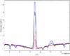 |
Fig. 1 Emission reversal in the Ca II H line in the average spectra of (from the less to the more active) Gl 581 (M3, in magenta), Gl 667C (M1.5, in pink), Gl 433 (M1.5, in yellow), Gl 176 (M2.5, dark), and Gl 674 (M3, in blue). Within our 100 M dwarf sample, Gl 581 has one of the weakest Ca II emission and illustrates a very quiet M dwarf. Gl 674 and Gl 176 have much stronger emission and are both moderately active with an identified rotational period of respectively 35 and 39 days (Bonfils et al. 2007; Forveille et al. 2009). |
3.1. Gl 433: Metallicity, activity, and dynamic population
According to the photometric calibration relation of Bonfils et al. (2005a), we estimated the metallicity of Gl 433 to be [Fe/H] ~ −0.2. This relation is based on a few stars with quite high metallicities, but Neves et al. (2012) show that for such value of [Fe/H] the calibration is correct with a typical dispersion of 0.2 dex. This is confirmed by the value of [Fe/H] = −0.13 obtained when using the Neves et al. (2012) relationship, itself an update of that from Schlaufman & Laughlin (2010). We conclude that Gl 433 is either solar or slightly sub-metallic.
Gl 433 is dynamically classified as a member of the old disk (Leggett 1992). Ca II H and K chromospheric emission is determined by Rauscher & Marcy (2006) and Gl 433 is in the least active half of M dwarfs of the same luminosity. For objects of similar spectral type, a direct comparison of Ca II emission lines gives the relative estimation of the rotational period (larger Ca II emissions correspond to shorter rotational periods). In Fig. 1, we present an average HARPS spectrum of Gl 433 in the region of the Ca II H line. Gl 433 has slightly stronger Ca II emission than Gl 581 (a very quite M dwarf), but far weaker than those of Gl 176 and Gl 674, whose rotational periods of 35 and 39 days were determined by Bonfils et al. (2007) and Forveille et al. (2009), respectively. The five M dwarfs of the Fig. 1 do not have identical spectral types (from M 1.5 to M 3), therefore the estimation of their rotation from the Ca II emission is only illustrative and shows that Gl 433 rotates most probably with a period longer than Gl 176 and Gl 674.
The X-ray flux of Gl 433 was not detected by ROSAT and we used a ROSAT limiting sensitivity of 2.5 × 1027 [d/10 pc] 2 erg/s (Schmitt et al. 1995) to estimate RX = Log LX/LBOL < −4.8. For an M dwarf of ~0.5 M⊙, the RX versus rotation period relation of Kiraga & Stepien (2007) give Prot > 40 days for such a level of X-ray flux. This lower limit to the rotation period is consistent with the estimate from the Ca II emission.
3.2. Gl 667C: Multiplicity, metallicity, activity and dynamic population
Gl 667C is the lightest and isolated component of a hierarchical triple system, the two other components being a closest couple of K dwarfs. Gl 667AB has a projected separation of 1.82′′, a period of 42.15 years, and a total dynamically determined mass of 1.27 M⊙ (Söderhjelm 1999). Gl 667C is at a projected distance of 32.4′′ of Gl 667AB, giving an expected semi-major axis of ~300 AU (for a distance of 7.23 pc and a factor of 1.26 between the expected and projected semi-major axis, Fischer & Marcy 1992).
The Bonfils et al. (2005a) photometric relationship for Gl667C gives us an estimate of the metallicity of –0.55 dex, which agrees quite well with the spectroscopic determination of [Fe/H] ~ −0.6 for the primary (Perrin et al. 1988; Zakhozhaj & Shaparenko 1996). This demonstrates that the Bonfils et al. (2005a) photometric calibration gives excellent results for low-metallicity M dwarfs. The Neves et al. (2012) relationship gives [Fe/H] ~ − 0.45, confirming that this star is a metal-poor M dwarfs.
In agreement with this chemical composition, Gl667 is classified as a member of the old disk population from its UVW velocity (Leggett 1992) and is among the objects of lower chromospheric emission for its luminosity (Rauscher & Marcy 2006). In Fig. 1, the Ca II H line emission of Gl 667C is slightly weaker than that of Gl 433, which is also indicative a long rotational period.
In the NEXXUS database (Schmitt & Liefke 2004), two different detections of the X-ray emission of Gl 667C are listed with one decade of difference. The ROSAT All-Sky Survey (RASS) value of log LX = 27.89 erg/s is the total flux for Gl 667ABC, whereas the value of the ROSAT High Resolution Imager (HRI) of log LX = 26.87 erg/s is a resolved measurement. This last measurement implies that RX = Log LX/LBOL = − 5.14 and that the rotational period is larger than 80 days (according to the Kiraga & Stepien (2007)RX versus rotational period relationship for a star of ~0.3 M⊙).
4. Orbital analysis of Gl 433
4.1. HARPS measurements
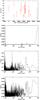 |
Fig. 2 From top to bottom: (1) HARPS RV data for Gl 433; (2) window function of the measurement; (3) periodogram of the HARPS measurements; and (4) periodogram of the residuals after substraction of the 7.3 day period. |
We obtained 67 RV measurements of Gl433 spanning 2904 days from December 2003 to November 2011. These data add 17 new points to those analyzed in Bonfils et al. (2013) and extend their time span by 1200 days. We estimated that the uncertainties of ~1.1 m/s are dominated by photon noise (the median S/N per pixel at 550 nm is 57). The RVs have an overall rms = 3.14 m/s and  per degree of freedom, confirming that there is variability in excess of the measurement uncertainties.
We therefore continued with a classical periodicity analysis, based on floating-mean periodograms (Gilliland & Baliunas 1987; Zechmeister et al. 2009). Figure 2 (third panel) depicts the periodogram of our RV time series and shows a strong power excess around the period of 7.3 days. We plot the window function in Fig. 2 (second panel) to identify the signal aliasing between the typical time sampling and the RV variability period. We adopted the normalization of periodograms proposed by Zechmeister et al. (2009), which is such that a power of one means that a sine function is a perfect fit to the data, whereas a power of zero indicates no improvement over a constant model. Hence, the most powerful peak was measured at a period of P ~ 7.3 days with a power pmax = 0.51, another peak appears at P ~ 1 day, it is the signal aliasing between the 7.3 day period and the 1 day time sampling which is clearly visible in the window function. To assess its signifiance we performed a bootstrap randomization (Press et al. 1992): we generated 10 000 virtual data sets by shuffling the actual RVs and retaining their dates, and for each set we computed a periodogram; using all periodograms we built a distribution of power maxima. In random sets it appears that power maxima exceed p = 0.40 only once every 100 trials, and never exceed p = 0.43 over 10 000 trials. This suggests a false alarm probability (FAP) < 1/10 000 for the 7.3-d period seen in the original periodogram. Moreover, for a more precise estimate of this low FAP value, we made use of the Cumming (2004) analytic formula FAP = M(1 − pmax)(N − 3)/2, where M is the number of independent frequencies in the periodogram, pmax its highest power value, and N the number of measurements. We approximated M by 2904/1 (the ratio of the time span of our observations to the typical 1-day sampling), and obtained the very low FAP value of 4 × 10⁻⁷.
We modeled the first periodic signal by a Keplerian orbit. Even though the periodicity was securely identified we used Yorbit (an heuristic algorithm, mixing standard non-linear minimisations and genetic algorithms; Ségransan et al., in prep; Bonfils et al. 2013) and benefited from a global search without any a priori. We converged on a period P = 7.3732 ± 0.0023 d, semi-amplitude K1 = 2.99 ± 0.38 m/s, and eccentricity e = 0.17 ± 0.13, which, for M⋆ = 0.48 M⊙ converts to msini = 5.49 ± 0.70 M⊕ (Table 2). The rms and  around the solution decreased to 2.17 m/s and 2.00 ± 0.09 per degree of freedom, respectively.
Inspecting the residuals and their periodogram (Fig. 2 bottom panel), we measured the power of the most powerful peak (~2000–3000 d; pmax = 0.28) and applied bootstrap randomization to find it was insignificant (FAP = 22%). We nevertheless found that adding a quadratic drift to the 1-planet model did improve the solution (rms = 1.91 m/s and  per degree of freedom).
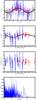 |
Fig. 3 Two-planet model of HARPS (in red) and UVES (in blue, from Zechmeister et al. 2009) RV measurements for Gl 433. Top: phased RV for a planet of 7.37 day period. Middle: radial velocity curve for the 3700 day period. Bottom: residuals and their periodogram. |
4.2. HARPS and UVES measurements
Fifty-four RV measurements of Gl 433 were also obtained with UVES by Zechmeister et al. (2009). They spanned 2553 days between March 2000 and March 2007 and therefore extended the time span of our observations by more than three years (see Fig. 3 – second panel). The mean RV measurement errors in the UVES data are 3.6 m/s, as indicated in Table 4 of Zechmeister et al. (2009). This team has demonstrated its ability to achieve an RV accuracy of ~3 m/s (including potential systematic errors) in the more stable M dwarfs of their program.
Hence, we combined the UVES and HARPS data (by adding a free parameter to the Keplerian fit to take into account an offset between the two datasets) and performed again a 1 planet fit with Yorbit. We converged on the same solution with more precise orbital parameters (P = 7.37131 ± 0.00096 d; K1 = 2.846 ± 0.248 m/s; e = 0.13 ± 0.09). The residuals around the solution show a power excess at P ~ 2857 d (pmax = 0.19) that appears to be significant. With 10 000 trials of bootstrap randomization, we found a FAP ~ 0.2%. Although signal, which is mainly due to the UVES data, needs to be confirmed with additional measurements, it justified the addition of a second planet to our model.
With a model composed of two planets on Keplerian orbits, Yorbit converges on periods of 7.37029 ± 0.00084 days and 3690 ± 250 days, with semi-amplitudes of 3.113 ± 0.224 m/s and 3.056 ± 0.433 m/s and eccentricities 0.08277 ± 0.07509 and 0.17007 ± 0.09428 (see Table 3 for the full set of parameters). The solution has an rms = 2.39 m/s and a  per degree of freedom, showing that the combination of the HARPS and UVES data sets have largely improved the parameter uncertainties.
4.3. The planetary system around Gl 433
In the past, Gl 433 was announced to host a brown dwarf of 30 Jupiter mass with an orbital period of ~500 days based on the astrometric measurements of Bernstein (1997). However all RV measurements that have since been published, including the present one, reject this detection.
Apparent Doppler shifts may also originate from stellar surface inhomogeneities, such as plages and spots, which can break the balance between light emitted in the red-shifted and the blue-shifted parts of a rotating star (e.g. Saar & Donahue 1997; Queloz et al. 2001; Desort et al. 2007). However, the long rotation period (>40 days) of Gl 433 ensures that its observed Doppler shift of 7.37 days does not originate from the stellar activity. A search for a correlation between the 7.37 day RV period and Hα, CaII-index, or bisector in our HARPS data yields a non-detection. Such signal is easily detected when the RV variation is due to activity for a period of ~35 days (and a fortiori for all shorter periods) (see the cases of Gl 176 and Gl 674; Bonfils et al. 2007; Forveille et al. 2009). This is strong evidence that the ~7 d period is not due to stellar surface inhomogeneities but to the presence of a planet orbiting around Gl 433.
This planet, Gl 433b, belongs to the category of super-Earths with a minimum mass of ~5.8 M⊕. At a separation of 0.058 AU from its star, Gl 433b is illuminated by a bolometric flux, per surface unity, ten times higher than what the Earth receives from the Sun.
The long-period variability detected in the UVES data set, may have several origins. Firstly, because the signal is detected only during one period, it should be confirmed by monitoring over a longer time period. If confirmed, the signal may originate from a ~10-year period planet of 50 M⊕. An alternative origin may be the effect of a long-term stellar magnetic cycle, like the so-called 11-year solar cycle, during which the fraction of the stellar disk covered by plages varies. In this region, the magnetic field attenuates the convective flux of the blueshifted plasma and impacts the mean observed RV on the order of few m/s or more (Meunier et al. 2010). Gomes da Silva et al. (2011) detect long-period variations for numerous activity proxies (CaII, NaI, HeI, Hα lines) of Gl 433 consistent with a period of ~10 years. The long periode RV variability is well-correlated with these activity proxies (Gomes da Silva et al. 2012). We therefore favor a magnetic cycle as the origin of the long-term signal.
5. Orbital analysis of Gl 667C
We obtained 179 measurements of Gl 667C RV spanning 2657 days between June 2004 and September 2011. The data add 36 points to those analyzed in Bonfils et al. (2013) and extend their time span by 1070 days. They have uncertainties of ~1.3 m/s (dominated by photon noise) and both rms and  values (resp. 4.3 m/s and 3.04 per degree of freedom) that indicate a variability above those uncertainties. All RVs are shown as a function of time in Fig. 4 (top panel), whereas their window function and floating-mean periodogram are presented in Fig. 5 (top two panels).
5.1. A one-planet and linear-fit solution
The long-term drift seen in Gl 667C RVs agrees well with the line-of-sight acceleration induced by its companion stellar pair Gl 667AB, which is about  m/s/yr (for a total mass MAB of 1.27 M⊙ and a separation of ~300 AU). Even without removing this linear drift, the periodogram show an additionally peak at P ~ 7.2 days (see Fig. 5, panel b). We removed an adjusted drift (
 m/s/yr) to make the periodic signal even stronger (pmax = 0.53; Fig. 5 panel c). To measure the FAP of the 7.2 day signal, we ran 10 000 bootstrap randomization and found no power stronger than 0.18, suggesting a FAP ≪ 1/10 000. We also computed the FAP with the Cumming (2004) prescription FAP = M(1 − pmax)(N − 5)/2. We approximated M by 2657/1 (the ratio of the time span to the typical sampling of our observations) and obtained the extremely low FAP value of ~10-25. We note that, in Fig. 5 (panel c), a significant and much less powerful peak is seen around P = 1.0094 day that corresponds to an alias of the 7.2-day peak for the typical ~1 day sampling.
We continued our analysis by adjusting with Yorbit the RVs to a model composed of one planet plus a linear drift and achieved a robust convergence for the orbital elements reported in Table 5. This model reduced the rms and per degree of freedom to 2.51 m/s and 2.02, respectively. Nevertheless these values remain above the photon noise and instrumental uncertainties, which prompted us to continue the analysis with the residuals and try more complex models.
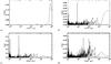 |
Fig. 5 a) Window function of the RV measurement; b) periodograms of the Gl 667C RV measurements; c) periodograms of the Gl 667C RV measurements after a drift removal; d) periodograms of the residual after subtraction of a drift + one planet model. |
5.2. A multi-Keplerian plus a linear fit solution
Following up on the periodogram of the residuals around the 1 planet + drift model (Fig. 5 panel d), we observed an additional power-excess around a series of periods, the six most powerful peaks being around 28, 91, 105, 122, 185, and 364 d, with p = 0.225, 0.215, 0.185, 0.181, 0.134, and 0.123, respectively. A bootstrap randomization indicates FAPs lower than 1/10 000 for the four most powerful peaks, whereas Cumming’s prescription attributes them a FAP < 10-12.
To model the RVs with a 2 planets + 1 drift model, one could pick the most powerful peak as a guessed period and perform a local minimization to derive all orbital parameters. We found however that this is not the most appropriate approach here because some of the less powerful peaks actually correspond to a signal with high eccentricities, and eventually turned to be better fit. To explore the best-fit solutions we generally prefer the global search implemented in Yorbit where the eccentricities are left to vary freely. We identified several solutions with similar values, reported in Table 5. For all solutions, the first planet and the linear drift had similar parameter values (see Sect. 5.1). On the other hand, the different solutions are discriminated by different orbital periods for the second planet, with Pc equals to ~28, 90, 106, 124, 186, or 372 days.
Six commensurable solutions (with similar reduced ) for the 2-Keplerian orbit + 1 drift model.
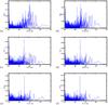 |
Fig. 6 Periodograms for the Gl 667C residual of radial velocity measurements after subtraction of a drift plus a two-planet solution. For all the panels, the period of the first planet is Pb = 7.2 days. From the left to the right and from the top to the bottom, the period of the second planet is Pc = 28,90,106,124,186, and 372 days. |
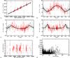 |
Fig. 7 Decomposition of our nominal three planet + 1 drift model for Gl 667C. Panel a) shows the contribution of the long-term drift with the three Keplerian contributions removed. Panels b), c), and d) show respectively radial velocity curves for Keplerians Pb = 7.2 d, Pc = 28.1 d, and Pd = 106.4 d. Residuals of this solution are shown in panel e) and their periodogram in panel f). |
To understand these signals, we analyzed the periodograms of the residuals around each solution. One the one hand, we found that for the solution with Pc = 28 d, the periodogram of the residual shows all the remaining peaks at 91, 105, 122, 185, and 364 days (Fig. 6 – panel a). On the other hand, when the solution is for any of the other periods Pc = 90, 106, 124, 186, or 372 d, then only the 28 d peak remains (e.g. Fig. 6 – panels b, c, d, e, and f). This means that all peaks at 90, 106, 120, 180, and 364 days actually correspond to a single signal, with its harmonics and aliases, and that the peak around 28 d is another independent signal.
One of the four signals identified so far (three periodic signals + one linear drift) have ambiguous solutions. Among the possible periods, the ~106-d period seems to correspond to the rotational period of the star as seen in one activity indicator (see Sect. 5.3). Conservatively, we continued by assuming that the signal is due to activity and used the 106-d period to obtain our fiducial solution. That assumption is given further credit when we run Yorbit. Without any a priori on any signal, Yorbit converges on a solution with P = 7.2,28, and 106 d. We present the orbital parameters of a 3 planets + 1 drift model in Table 6 and the RV decomposition and periodogram of the residuals around that solution in Fig. 7. That solution has an rms and equal to 1.73 m/s and 1.44 ± 0.06 per degree of freedom, respectively.
Finally, we inspected the residuals around the last model (see panels (e) and (f) in Fig. 7). We found the power maximum of the periodogram located around P = 1.0083 d (a possible 1-day alias with a period of 121 days) with a power pmax = 0.13, to which we attributed a FAP of 2.8%. We therefore did not consider that a significant sine signal remains in the data. We plan to accumulate more RVs to check wether this signal corresponds to either i) an additional companion; ii) an alias of (improperly corrected) stellar activity of longer timescale; or iii) noise.
5.3. The planetary system around Gl 667C
To assess whether one of the radial velocity periodic signal could be due to stellar rotation, we searched for periodicity in several activity diagnostics (Hα and CaII-index and the bisector-inverse slope (BIS) and full-width at half-maximum (FWHM) of the cross-correlation function). The clearest signal detected is a very strong peak in the periodogram of the FWHM at a period of ~105 days with a FAP lower than 0.1% (see Fig. 8).
The periodic variation in the FWHM is an estimate of the rotation (Queloz et al. 2009). A rotational period of ~105 days for Gl 667C is consistent with the faint activity level of these stars discussed in Sect. 3.2 and such a period matches one of the power excess seen in our RV periodogram analysis. Thus, our favorite explanation is that the period of ~105 days and all its harmonics or aliases at P = 90, 124, 186, and 372 days (see Sect. 5.2) are due to stellar rotation. However, we tried to use different subsets of RV points and found that the best solution may appear with Pd = 90, 106, or 186 d. We therefore considered that the RV signal with a long (P > 90 days) period has an uncertain origin of possibly stellar rotation (the most probable in our point of view), or either a high-eccentricity planet, two planets in resonance or a combination of these explanations.
The RV signals at 7.2 d and 28.1 d are completely independent of the long period ones and cannot be due to stellar rotation. Thus, at least two super-Earths are present at close separation to Gl 667C that have a masses of 5.5 M⊕ and 4.25 M⊕. As previously announced by our team in Bonfils et al. (2013) with GTO-HARPS data, the use of supplementary HARPS RV data allows us to specify their parameters. At a separation of 0.05 and 0.12 AU from their star, Gl 667Cb and Gl 667Cc are respectively illuminated by a bolometric flux, per unit area, 5.51 and 0.89 times than that the Earth receives from the Sun (in using the stellar luminosity of Table 1). The super-Earth Gl 667Cc is then in the middle of the habitable zone of its star. We discuss this point in detail in the next section.
6. A planet in the middle of the habitable zone of an M dwarf
6.1. Gl 667Cc
Super-Earths in the habitable zone of their host stars, which by definition is the region where liquid water can be stable on the surface of a rocky planet (Huang 1959; Kasting et al. 1993), currently garner considerable interest. For a detailed discussion of the HZ, we refer the reader to Selsis et al. (2007) or Kaltenegger & Sasselov (2011) but summarize their most salient points. One important consideration is that planets with masses outside the 0.5–10 M⊕ range cannot host liquid surface water. Planets of mass lower than this range have too weak a gravity to retain a sufficiently dense atmosphere, and those above the upper end of the range accrete a massive He-H envelope. In either case, the pressure at the surface cannot support liquid water. The 10 M⊕ upper limit is somewhat fuzzy, since planets in the 3–10 M⊕ range can have very different densities (reflecting their different structures) for a given mass: Earth-like, Neptune-like, and ocean planets can all exist for the same mass (e.g. Fig. 3 in Winn et al. 2011).
Three Keplerian + 1 linear-drift orbital solution.
To potentially harbor liquid water, a planet with a dense atmosphere such as the Earth needs an equilibrium temperature between 175 K and 270 K (Selsis et al. 2007; Kaltenegger & Sasselov 2011, and references therein). If Teq > 270 K, a planet with a water-rich atmosphere will experience a phase of a runaway greenhouse effect (see Selsis et al. 2007). At the other end of the range, CO2 will irreversibly freeze out from the atmosphere of planets with Teq < 175 K, preventing a sufficient greenhouse effect to avoid the freezing of all surface water. Either case obviously makes the planet uninhabitable. The inner limit of the habitable zone is well-constrained. The outer one, by contrast, is very sensitive to the complex and poorly constrained meteorology of CO2 clouds, through the balance between their reflecting efficiency (which cools the planet) and their greenhouse effect (which warms it) (Forget & Pierrehumbert 1997; Mischna et al. 2000; Selsis et al. 2007). Finally, a location inside the habitable zone is a necessary condition for hosting surface water, but by no means a sufficient one: the long-term survival of surface water involves complex ingredients such as a carbonate-silicate geological cycle and an adequate initial H2O supply.
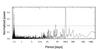 |
Fig. 8 Periodogram for the FWHM of the correlation peak for the Gl 667C HARPS measurements. A peak at ~105 days is clearly visible and interpreted as the rotational period of Gl 667C. The line show the 10% and 1% FAP levels. |
Adopting the notations of Kaltenegger et al. (2011), the equilibrium temperature of a planet is: 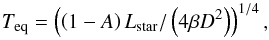 (1)where Lstar is the bolometric luminosity of the star, D is the planet’s semi-major axis, β is the geometrical fraction of the planet surface that re-radiates the absorbed flux (β = 1 for a rapidly rotating planet with a dense atmosphere, such as the Earth; β = 0.5 for an atmosphere-less planet that always show the same side to its star), and A the wavelength-integrated Bond albedo. Using the stellar parameters of Table 1, the equilibrium temperatures of Gl433b and Gl667Cb are respectively 495
 K and 426 K. Both planets are firmly in the hot super-Earth category. In contrast, Gl 667Cc has
  K, which should be compared to
  K for the Earth.
The three dimensional (3D) atmospheric models of Heng et al. (2011a,b) suggest that a planet like Gl667Cc most likely has β close to 1, even when it is tidally locked and always shows the same hemisphere to its star, since they find that a modestly dense Earth-like atmosphere ensures a full re-distribution of the incoming energy. This conclusion, a fortiori, also applies to the presumably denser atmosphere of a 4.25 M⊕ planet (Wordsworth et al. 2011). With Teq ~ 270(1 − A)1/4 K, Gl667Cc is therefore in the HZ for any albedo in the [0–0.83] range.
Detailed 3D atmospheric simulations (e.g. Wordsworth et al. 2011; Heng & Vogt 2011) will need to be tuned to the characteristics of Gl 667Cc to ascertain its possible climate. In the mean time, this planet, which receives from its star 89% of the bolometric solar flux at Earth, is a very strong habitable-planet candidate.
6.2. Particularity of the habitable zone around M dwarfs
Two main differences between planets in the HZ of solar-like stars and M dwarfs are often pointed out. Firstly, a planet in the HZ of an M dwarf is closer to its star, and therefore subject to more intense tidal forces. As a result, it is likely to quickly be captured into a spin-orbit resonance. The solar system demonstrates, however, that this does not necessarily imply that it will be forced into synchronous rotation. The final equilibrium rotation of a tidally influenced planet depends on both its orbital eccentricity and the density of its atmosphere (Doyle et al. 1993; Correia et al. 2008; Correia & Laskar 2010; Heller et al. 2011). Mercury, for instance, has been captured into the 3:2, rather than 1:1, spin-orbit resonance (Correia & Laskar 2004), and Venus has altogether escaped capture into a resonance because thermal atmospheric tides counteract its interior tides (Correia & Laskar 2003). Whatever the final spin-orbit ratio, the tidal forces will influence both the night and day successions, and therefore the climate. As discussed above however, energy redistribution by an atmosphere at least as dense as that of the Earth is efficient (Wordsworth et al. 2011; Heng et al. 2011b,a), and will prevent glaciation and atmospheric collapse on the night side.
The second major difference is in the stellar magnetic activity, owing to its dependence on stellar mass. M dwarfs, on average, are much more active than solar-like stars. This results from the combination of two effects: lower mass stars have much longer braking times for stellar rotation (Delfosse et al. 1998; Barnes 2003; Delorme et al. 2011), and for the same rotation period they are more active (Kiraga & Stepien 2007). As a result, a planet in the HZ of an early M dwarf receives intense X-ray and UV radiation for ten times longer than the ~100 Myr that the Earth spent close to a very active Sun (Ribas et al. 2005; Selsis et al. 2007). Stellar X-ray and UV radiation, as well as coronal mass ejections (CMEs), could potentially cause a major atmospheric escape (see Scalo et al. 2007; Lammer et al. 2009, for reviews).
Several theoretical studies have looked into the evolution of planetary atmospheres in the M-dwarf HZ to investigate whether they lose essential chemical species, such as H2O, and may even be completely eroded? The problem is complex, with many uncertain parameters, and the range of possible answers is very wide. Amongst other uncertain factors, the escape ratio sensitively depends on (1) the intensity and frequency of CMEs for M dwarfs, which is poorly known, and may be much smaller that initially claimed (van den Oord & Doyle 1997; Wood et al. 2005); (2) the magnetic moment of the planet (a strong magnetosphere will protect the planet against CME-induced ion pick up Lammer et al. 2007); and (3) details of the atmospheric chemistry and composition (through atmosphere-flare photo-chemical interaction Segura et al. 2010 and IR radiative cooling from the vibrational-rotational band Lammer et al. 2007). In two limiting cases of planets in M-dwarfs HZ, Lammer et al. (2007), conclude that the atmosphere of an unmagnetized Earth-mass planet can be completely eroded during the Gyr-long active phase of its host star, while Tian (2009) finds that the atmosphere of a seven Earth-mass super-Earth is stable even around very active M dwarfs, especially if the atmosphere mostly contains CO2. The continuous outgassing of essential atmospheric species from volcanic activity can, of course, also protect an atmosphere by compensating for its escape.
These differences imply that a planet in the habitable zone of an M dwarf is unlikely to be a twin of the Earth. Habitability however is not restricted to Earth twins, and Barnes et al. (2011) conclude that “no known phenomenon completely precludes the habitability of terrestrial planets orbiting cool stars”. A massive telluric planet, such as Gl667Cc (M2sini = 4.25 M⊕), most likely has a massive planetary core, and as a consequence a stronger dynamo and more active volcanism. Both factors help to protect against atmospheric escape, and super-Earths may perhaps be stronger candidates for habitability around M dwarfs than true Earth-mass planets.
6.3. Comparing Gl 667Cc with other known planets in the habitable zone
HARPS has previously discovered two planets inside the HZs of the stars Gl 581 and HD85512. Gl 581d (Udry et al. 2007; Mayor et al. 2009) (M2sini = 7 M⊕) receives from its M3V host star just ~25% of the energy that the Earth receives from the Sun, and is thus located in the outer habitable zone of its star. Detailed models (Wordsworth et al. 2011) confirm that Gl 581d can have surface liquid water for a wide range of plausible atmospheres. HD85512b (Pepe et al. 2011) is a M2sini = 3.5 M⊕ planet in the inner habitable zone of a K5-dwarf that receives about twice as much stellar energy as the Earth. It could harbor surface liquid water if at least 50% of its surface is covered by highly reflective clouds (Kaltenegger et al. 2011).
Vogt et al. (2010) announced another super-Earth in the HZ of Gl 581, which they found in an analysis combining HARPS and HIRES RV data. The statistical significance of this detection has, however, been questioned (e.g. Tuomi 2011), and an extended HARPS dataset now demonstrates that the planet is unlikely to exist with the proposed parameters (Forveille et al. 2011).
Borucki et al. (2011) announced six planetary candidates in the HZ of Kepler targets with a radius smaller than twice that of Earth, which they adopted as a nominal limit between telluric and Neptune-like planets. Kaltenegger & Sasselov (2011) reduce this number to three HZ planetary candidates, by discarding three planets that they find are too hot to host water if their coverage by reflective clouds is under 50%. Borucki et al. (2012) confirmed that Kepler 22b (listed as KOI-87.01 in Borucki et al. 2011) is a planet, making it the first planet with a measured radius orbiting in a habitable zone. Kaltenegger & Sasselov (2011) however discarded Kepler 22b from their candidate list because its radius is above two Earth-radii.
To summarize, two planets with measured minimum masses in the range for telluric planets (Gl 581d and HD 85512b) are known to orbit in the HZ of their respective stars. Another one, with a measured radius slightly above the nominal limit for a rocky planet, orbits at a similar location (Kepler 22b). Finally, three Kepler candidates with radii corresponding to telluric planets and positions in habitable zones currently await confirmation. Gl 667Cc, announced in Bonfils et al. (2013) and discussed in detail here, is actually the most promising of these for holding conditions compatible with surface liquid water. Receiving ~10% less stellar energy than the Earth and with a minimum mass of M2sini = 4.25 M⊕, it is very likely to be a rocky planet in the middle of the habitable zone of its star.
7. Summary and conclusions
We have analyzed in detail three super-Earths announced in Bonfils et al. (2013): Gl 433b, Gl 667Cb and Gl 667Cc. One, Gl667Cc, is a M2sini = 4.25 M⊕ planet in the middle of the habitable zone of a M1.5V star. It is to date the extra-solar planet with the closest characteristics to the Earth, but does not approach being an Earth twin. Its main differences from Earth are its significantly higher mass and different stellar environment, which might potentially can have caused its different evolution.
Host stars of giant planets are preferentially metal-rich (e.g. Santos et al. 2001, 2004; Fischer & Valenti 2005). In contrast, the detection rate of planets with masses lower than 30–40 M⊕ does not clearly correlate with stellar metallicity (Mayor et al. 2011). These results make the discovery of two super-Earths around Gl 667C ([Fe/H] ~ − 0.6, Sect. 3) less surprising, but this star remains one of the most metal-poor planetary host stars known to date, with just six planetary host stars listed having a lower metallicity in the Extrasolar Planets Encyclopaedia1 (Schneider et al. 2011). The metallicity of Gl 433, [Fe/H] ~ − 0.2, is close to the median value of the solar neighborhood, and therefore unremarkable.
The planets Gl 667Cb and c orbit the outer component of a hierarchical triple system. Fewer than ten other planetary systems, listed in Desidera et al. (2011), share this characteristic. These authors conclude that planets occur with similar frequencies around the isolated component of a triple system and around single stars. The planets around Gl 667C, however, are unusual in orbiting the lowest-mass component of the system.
The three planets discussed here enter in our Bonfils et al. (2013) statistical study, which establishes that super-Earths are very common around M dwarfs. Our HARPS survey of ~100 stars has, in particular, found two super-Earths in habitables zones, Gl 581d and Gl 667Cc, even though both planets are located in parts of the mass-period diagram where its detection completeness is lower tan 10 percent. This clearly indicates that super-Earths are common in the habitable zones of M dwarfs, with a 42 frequency (Bonfils et al. 2013). Future instruments optimized for planet searches around M dwarfs, such as the SPIRou (on CFHT) and CARMENES (at Calar Alto observatory) near-IR spectrographs, will vastly increase our inventory of such planets around nearby M dwarfs. Theses instruments should be able to identify ~50–100 planets in the habitable zones of M-dwarfs, and with a ~2% transit probability for these, to find at least one transiting habitable planet around a bright M dwarf. Such a radial-velocity educated approach has already been undertaken with HARPS (Bonfils et al. 2011) and led to the discovery of GJ3470b (Bonfils et al. 2012). In this context, we stress that a photometric search for transits must soon be carried out for Gl 667Cc, for which there is a ~1.5% probability of transits occuring.
Online material
Appendix A: Radial velocity measurements
Acknowledgments
We thank the 3.6-m team for their support during the observations which produced these results. We thank Abel Méndez and Franck Selsis for their helpful discussion about the “habitability” of Gl 667Cc, and Carolin Liefke for reporting to us that a resolved ROSAT measurement existed for Gl667C. We would like to thank an anonymous referee for his/her comments, which helped to clarify the paper. Financial support from the “Programme National de Planétologie” (PNP) of CNRS/INSU, France, is gratefully acknowledged. N.C.S. acknowledges the support of the European Research Council/European Community under the FP7 through Starting Grant agreement number 239953, and from Fundação para a Ciência e a Tecnologia (FCT) through program Ciência 2007, funded by FCT (Portugal) and POPH/FSE (EC), and in the form of grants reference PTDC/CTE-AST/098528/2008 and PTDC/CTE-AST/098604/2008. V.N. would also like to acknowledge the support of the FCT in the form of the fellowship SFRH/BD/60688/2009.
References
- Anglada-Escudé, G., Arriagada, P., & Vogt, S. S. 2012, ApJ, 751, L16 [NASA ADS] [CrossRef] [Google Scholar]
- Barnes, S. A. 2003, ApJ, 586, 464 [NASA ADS] [CrossRef] [Google Scholar]
- Barnes, R., Meadows, V. S., Domagal-Goldman, S. D., et al. 2011, in 16th Cambridge Workshop on Cool Stars, Stellar Systems, and the Sun, eds. C. Johns-Krull, M. K. Browning, & A. A. West, ASP Conf. Ser., 448, 391 [Google Scholar]
- Batalha, N. M., Borucki, W. J., Bryson, S. T., et al. 2011, ApJ, 729, 27 [NASA ADS] [CrossRef] [Google Scholar]
- Bernstein, H. 1997, in Hipparcos – Venice ’97, eds. R. M. Bonnet, E. Høg, P. L. Bernacca, et al., ESA SP, 402, 705 [Google Scholar]
- Bonfils, X., Delfosse, X., Udry, S., et al. 2005a, A&A, 442, 635 [NASA ADS] [CrossRef] [EDP Sciences] [Google Scholar]
- Bonfils, X., Forveille, T., Delfosse, X., et al. 2005b, A&A, 443, L15 [NASA ADS] [CrossRef] [EDP Sciences] [Google Scholar]
- Bonfils, X., Mayor, M., Delfosse, X., et al. 2007, A&A, 474, 293 [NASA ADS] [CrossRef] [EDP Sciences] [Google Scholar]
- Bonfils, X., Gillon, M., Forveille, T., et al. 2011, A&A, 528, A111 [NASA ADS] [CrossRef] [EDP Sciences] [Google Scholar]
- Bonfils, X., Gillon, M., Udry, S., et al. 2012, A&A, 546, A27 [NASA ADS] [CrossRef] [EDP Sciences] [Google Scholar]
- Bonfils, X., Delfosse, X., Udry, S. 2013, A&A, 549, A109 [NASA ADS] [CrossRef] [EDP Sciences] [Google Scholar]
- Borucki, W. J., Koch, D. G., Basri, G., et al. 2011, ApJ, 736, 19 [NASA ADS] [CrossRef] [Google Scholar]
- Borucki, W. J., Koch, D. G., Batalha, N., et al. 2012, ApJ, 745, 120 [NASA ADS] [CrossRef] [Google Scholar]
- Charbonneau, D., Berta, Z. K., Irwin, J., et al. 2009, Nature, 462, 891 [NASA ADS] [CrossRef] [PubMed] [Google Scholar]
- Correia, A. C. M., & Laskar, J. 2003, Icarus, 163, 24 [NASA ADS] [CrossRef] [Google Scholar]
- Correia, A. C. M., & Laskar, J. 2004, Nature, 429, 848 [NASA ADS] [CrossRef] [Google Scholar]
- Correia, A. C. M., & Laskar, J. 2010, in Tidal Evolution of Exoplanets, ed. S. Seager, 239 [Google Scholar]
- Correia, A. C. M., Levrard, B., & Laskar, J. 2008, A&A, 488, L63 [NASA ADS] [CrossRef] [EDP Sciences] [Google Scholar]
- Cumming, A. 2004, MNRAS, 354, 1165 [NASA ADS] [CrossRef] [Google Scholar]
- Cutri, R. M., Skrutskie, M. F., van Dyk, S., et al. 2003, 2MASS All Sky Catalog of point sources (Univ. of Massachusetts) [Google Scholar]
- Delfosse, X., Forveille, T., Perrier, C., & Mayor, M. 1998, A&A, 331, 581 [NASA ADS] [Google Scholar]
- Delfosse, X., Forveille, T., Ségransan, D., et al. 2000, A&A, 364, 217 [NASA ADS] [Google Scholar]
- Delorme, P., Collier Cameron, A., Hebb, L., et al. 2011, MNRAS, 413, 2218 [NASA ADS] [CrossRef] [Google Scholar]
- Demory, B.-O., Gillon, M., Deming, D., et al. 2011, A&A, 533, A114 [NASA ADS] [CrossRef] [EDP Sciences] [Google Scholar]
- Desidera, S., Carolo, E., Gratton, R., et al. 2011, A&A, 533, A90 [NASA ADS] [CrossRef] [EDP Sciences] [Google Scholar]
- Desort, M., Lagrange, A., Galland, F., Udry, S., & Mayor, M. 2007, A&A, 473, 983 [NASA ADS] [CrossRef] [EDP Sciences] [Google Scholar]
- Doyle, L., McKay, C., Whitmire, D., et al. 1993, in Third Decennial US-USSR Conference on SETI, ed. G. S. Shostak, ASP Conf. Ser., 47, 199 [Google Scholar]
- Fischer, D. A., & Marcy, G. W. 1992, ApJ, 396, 178 [NASA ADS] [CrossRef] [Google Scholar]
- Fischer, D. A., & Valenti, J. 2005, ApJ, 622, 1102 [NASA ADS] [CrossRef] [Google Scholar]
- Forget, F., & Pierrehumbert, R. T. 1997, Science, 278, 1273 [NASA ADS] [CrossRef] [PubMed] [Google Scholar]
- Forveille, T., Bonfils, X., Delfosse, X., et al. 2009, A&A, 493, 645 [NASA ADS] [CrossRef] [EDP Sciences] [Google Scholar]
- Forveille, T., Bonfils, X., Delfosse, X., et al. 2011, A&A, submitted [arXiv:1109.2505] [Google Scholar]
- Gilliland, R. L., & Baliunas, S. L. 1987, ApJ, 314, 766 [NASA ADS] [CrossRef] [Google Scholar]
- Gomes da Silva, J., Santos, N. C., Bonfils, X., et al. 2011, A&A, 534, A30 [NASA ADS] [CrossRef] [EDP Sciences] [Google Scholar]
- Gomes da Silva, J., Santos, N. C., Bonfils, X., et al. 2012, A&A, 541, A9 [NASA ADS] [CrossRef] [EDP Sciences] [Google Scholar]
- Hawley, S. L., Gizis, J. E., & Reid, I. N. 1996, AJ, 112, 2799 [NASA ADS] [CrossRef] [Google Scholar]
- Heller, R., Leconte, J., & Barnes, R. 2011, A&A, 528, A27 [NASA ADS] [CrossRef] [EDP Sciences] [Google Scholar]
- Heng, K., & Vogt, S. S. 2011, MNRAS, 415, 2145 [NASA ADS] [CrossRef] [Google Scholar]
- Heng, K., Frierson, D. M. W., & Phillipps, P. J. 2011a, MNRAS, 418, 2669 [Google Scholar]
- Heng, K., Menou, K., & Phillipps, P. J. 2011b, MNRAS, 413, 2380 [NASA ADS] [CrossRef] [Google Scholar]
- Huang, S.-S. 1959, PASP, 71, 421 [Google Scholar]
- Kaltenegger, L., & Sasselov, D. 2011, ApJ, 736, L25 [NASA ADS] [CrossRef] [Google Scholar]
- Kaltenegger, L., Udry, S., & Pepe, F. 2011, unpublished [arXiv:1108.3561] [Google Scholar]
- Kasting, J. F., Whitmire, D. P., & Reynolds, R. T. 1993, Icarus, 101, 108 [NASA ADS] [CrossRef] [PubMed] [Google Scholar]
- Kiraga, M., & Stepien, K. 2007, Acta Astron., 57, 149 [NASA ADS] [Google Scholar]
- Kürster, M., Endl, M., Rouesnel, F., et al. 2003, A&A, 403, 1077 [NASA ADS] [CrossRef] [EDP Sciences] [Google Scholar]
- Lammer, H., Lichtenegger, H. I. M., Kulikov, Y. N., et al. 2007, Astrobiology, 7, 185 [NASA ADS] [CrossRef] [PubMed] [Google Scholar]
- Lammer, H., Bredehöft, J. H., Coustenis, A., et al. 2009, A&ARv, 17, 181 [NASA ADS] [CrossRef] [Google Scholar]
- Léger, A., Rouan, D., Schneider, J., et al. 2009, A&A, 506, 287 [NASA ADS] [CrossRef] [EDP Sciences] [MathSciNet] [Google Scholar]
- Leggett, S. K. 1992, ApJS, 82, 351 [NASA ADS] [CrossRef] [Google Scholar]
- Leggett, S. K., Allard, F., Dahn, C., et al. 2000, ApJ, 535, 965 [NASA ADS] [CrossRef] [Google Scholar]
- Lissauer, J. J., Fabrycky, D. C., Ford, E. B., et al. 2011, Nature, 470, 53 [NASA ADS] [CrossRef] [PubMed] [Google Scholar]
- Lovis, C., & Pepe, F. 2007, A&A, 468, 1115 [NASA ADS] [CrossRef] [EDP Sciences] [Google Scholar]
- Mayor, M., Pepe, F., Queloz, D., et al. 2003, The Messenger, 114, 20 [NASA ADS] [Google Scholar]
- Mayor, M., Bonfils, X., Forveille, T., et al. 2009, A&A, 507, 487 [NASA ADS] [CrossRef] [EDP Sciences] [Google Scholar]
- Mayor, M., Marmier, M., Lovis, C., et al. 2011, A&A, submitted [arXiv:1109.2497] [Google Scholar]
- Meunier, N., Desort, M., & Lagrange, A. 2010, A&A, 512, A39 [NASA ADS] [CrossRef] [EDP Sciences] [Google Scholar]
- Mischna, M. A., Kasting, J. F., Pavlov, A., & Freedman, R. 2000, Icarus, 145, 546 [NASA ADS] [CrossRef] [PubMed] [Google Scholar]
- Morales, J. C., Ribas, I., & Jordi, C. 2008, A&A, 478, 507 [NASA ADS] [CrossRef] [EDP Sciences] [Google Scholar]
- Muirhead, P. S., Johnson, J. A., Apps, K., et al. 2012, ApJ, 747, 144 [NASA ADS] [CrossRef] [Google Scholar]
- Neves, V., Bonfils, X., Santos, N. C., et al. 2012, A&A, 538, A25 [NASA ADS] [CrossRef] [EDP Sciences] [Google Scholar]
- Pepe, F., Mayor, M., Galland, F., et al. 2002, A&A, 388, 632 [NASA ADS] [CrossRef] [EDP Sciences] [Google Scholar]
- Pepe, F., Lovis, C., Ségransan, D., et al. 2011, A&A, 534, A58 [NASA ADS] [CrossRef] [EDP Sciences] [Google Scholar]
- Perrin, M., Cayrel de Strobel, G., & Dennefeld, M. 1988, A&A, 191, 237 [NASA ADS] [Google Scholar]
- Perryman, M. A. C., Lindegren, L., Kovalevsky, J., et al. 1997, A&A, 323, L49 [NASA ADS] [Google Scholar]
- Press, W. H., Teukolsky, S. A., Vetterling, W. T., & Flannery, B. P. 1992, Numerical recipes in FORTRAN. The art of scientific computing, (New York: Cambridge University Press) [Google Scholar]
- Queloz, D., Henry, G. W., Sivan, J. P., et al. 2001, A&A, 379, 279 [NASA ADS] [CrossRef] [EDP Sciences] [Google Scholar]
- Queloz, D., Bouchy, F., Moutou, C., et al. 2009, A&A, 506, 303 [NASA ADS] [CrossRef] [EDP Sciences] [Google Scholar]
- Rauscher, E., & Marcy, G. W. 2006, PASP, 118, 617 [NASA ADS] [CrossRef] [Google Scholar]
- Ribas, I., Guinan, E. F., Güdel, M., & Audard, M. 2005, ApJ, 622, 680 [NASA ADS] [CrossRef] [Google Scholar]
- Saar, S. H., & Donahue, R. A. 1997, ApJ, 485, 319 [NASA ADS] [CrossRef] [Google Scholar]
- Santos, N. C., Israelian, G., & Mayor, M. 2001, A&A, 373, 1019 [NASA ADS] [CrossRef] [EDP Sciences] [Google Scholar]
- Santos, N. C., Israelian, G., & Mayor, M. 2004, A&A, 415, 1153 [NASA ADS] [CrossRef] [EDP Sciences] [Google Scholar]
- Scalo, J., Kaltenegger, L., Segura, A. G., et al. 2007, Astrobiology, 7, 85 [NASA ADS] [CrossRef] [PubMed] [Google Scholar]
- Schlaufman, K. C., & Laughlin, G. 2010, A&A, 519, A105 [NASA ADS] [CrossRef] [EDP Sciences] [Google Scholar]
- Schmitt, J. H. M. M., & Liefke, C. 2004, A&A, 417, 651 [NASA ADS] [CrossRef] [EDP Sciences] [Google Scholar]
- Schmitt, J. H. M. M., Fleming, T. A., & Giampapa, M. S. 1995, ApJ, 450, 392 [NASA ADS] [CrossRef] [Google Scholar]
- Schneider, J., Dedieu, C., Le Sidaner, P., Savalle, R., & Zolotukhin, I. 2011, A&A, 532, A79 [NASA ADS] [CrossRef] [EDP Sciences] [Google Scholar]
- Segura, A., Kasting, J. F., Meadows, V., et al. 2005, Astrobiology, 5, 706 [NASA ADS] [CrossRef] [PubMed] [Google Scholar]
- Segura, A., Walkowicz, L. M., Meadows, V., Kasting, J., & Hawley, S. 2010, Astrobiology, 10, 751 [NASA ADS] [CrossRef] [PubMed] [Google Scholar]
- Selsis, F., Kasting, J. F., Levrard, B., et al. 2007, A&A, 476, 1373 [NASA ADS] [CrossRef] [EDP Sciences] [Google Scholar]
- Söderhjelm, S. 1999, A&A, 341, 121 [Google Scholar]
- Tian, F. 2009, ApJ, 703, 905 [NASA ADS] [CrossRef] [Google Scholar]
- Tuomi, M. 2011, A&A, 528, L5 [NASA ADS] [CrossRef] [EDP Sciences] [Google Scholar]
- Udry, S., Bonfils, X., Delfosse, X., et al. 2007, A&A, 469, L43 [NASA ADS] [CrossRef] [EDP Sciences] [Google Scholar]
- van den Oord, G. H. J., & Doyle, J. G. 1997, A&A, 319, 578 [NASA ADS] [Google Scholar]
- Vogt, S. S., Butler, R. P., Rivera, E. J., et al. 2010, ApJ, 723, 954 [NASA ADS] [CrossRef] [EDP Sciences] [Google Scholar]
- Winn, J. N., Matthews, J. M., Dawson, R. I., et al. 2011, ApJ, 737, L18 [NASA ADS] [CrossRef] [Google Scholar]
- Wolfgang, A., & Laughlin, G. 2012, ApJ, 750, 148 [NASA ADS] [CrossRef] [Google Scholar]
- Wood, B. E., Müller, H.-R., Zank, G. P., Linsky, J. L., & Redfield, S. 2005, ApJ, 628, L143 [Google Scholar]
- Wordsworth, R. D., Forget, F., Selsis, F., et al. 2011, ApJ, 733, L48 [NASA ADS] [CrossRef] [Google Scholar]
- Zakhozhaj, V. A., & Shaparenko, E. F. 1996, Kinematika i Fizika Nebesnykh Tel, 12, 20 [Google Scholar]
- Zechmeister, M., Kürster, M., & Endl, M. 2009, A&A, 505, 859 [NASA ADS] [CrossRef] [EDP Sciences] [Google Scholar]
All Tables
Six commensurable solutions (with similar reduced ) for the 2-Keplerian orbit + 1 drift model.
All Figures
|
Fig. 1 Emission reversal in the Ca II H line in the average spectra of (from the less to the more active) Gl 581 (M3, in magenta), Gl 667C (M1.5, in pink), Gl 433 (M1.5, in yellow), Gl 176 (M2.5, dark), and Gl 674 (M3, in blue). Within our 100 M dwarf sample, Gl 581 has one of the weakest Ca II emission and illustrates a very quiet M dwarf. Gl 674 and Gl 176 have much stronger emission and are both moderately active with an identified rotational period of respectively 35 and 39 days (Bonfils et al. 2007; Forveille et al. 2009). |
| In the text | |
|
Fig. 2 From top to bottom: (1) HARPS RV data for Gl 433; (2) window function of the measurement; (3) periodogram of the HARPS measurements; and (4) periodogram of the residuals after substraction of the 7.3 day period. |
| In the text | |
|
Fig. 3 Two-planet model of HARPS (in red) and UVES (in blue, from Zechmeister et al. 2009) RV measurements for Gl 433. Top: phased RV for a planet of 7.37 day period. Middle: radial velocity curve for the 3700 day period. Bottom: residuals and their periodogram. |
| In the text | |
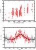 |
Fig. 4 Top: HARPS RV of Gl 667C. Bottom: one planet plus a linear drift model. |
| In the text | |
|
Fig. 5 a) Window function of the RV measurement; b) periodograms of the Gl 667C RV measurements; c) periodograms of the Gl 667C RV measurements after a drift removal; d) periodograms of the residual after subtraction of a drift + one planet model. |
| In the text | |
|
Fig. 6 Periodograms for the Gl 667C residual of radial velocity measurements after subtraction of a drift plus a two-planet solution. For all the panels, the period of the first planet is Pb = 7.2 days. From the left to the right and from the top to the bottom, the period of the second planet is Pc = 28,90,106,124,186, and 372 days. |
| In the text | |
|
Fig. 7 Decomposition of our nominal three planet + 1 drift model for Gl 667C. Panel a) shows the contribution of the long-term drift with the three Keplerian contributions removed. Panels b), c), and d) show respectively radial velocity curves for Keplerians Pb = 7.2 d, Pc = 28.1 d, and Pd = 106.4 d. Residuals of this solution are shown in panel e) and their periodogram in panel f). |
| In the text | |
|
Fig. 8 Periodogram for the FWHM of the correlation peak for the Gl 667C HARPS measurements. A peak at ~105 days is clearly visible and interpreted as the rotational period of Gl 667C. The line show the 10% and 1% FAP levels. |
| In the text | |
Current usage metrics show cumulative count of Article Views (full-text article views including HTML views, PDF and ePub downloads, according to the available data) and Abstracts Views on Vision4Press platform.
Data correspond to usage on the plateform after 2015. The current usage metrics is available 48-96 hours after online publication and is updated daily on week days.
Initial download of the metrics may take a while.